運用複雜度及亮度分佈檢測之建立在Boosting基礎上的車輛偵測

國

立

交

通

大

學

多媒體工程研究所

碩

士

論

文

運用複雜度及亮度分佈檢測之建立在 Boosting 基礎上的

車輛偵測

Robust Boosting Based Vehicle Detection with Complexity and Histogram

Verification

研 究 生：柯弼文

指導教授：林進燈 教授

運用複雜度及亮度分佈檢測之建立在 Boosting 基礎上的車輛偵測

Robust Boosting Based Vehicle Detection with Complexity and Histogram

Verification

研 究 生：柯弼文 Student：Be-Wen Ko

指導教授：林進燈 Advisor：Chin-Teng Lin

國 立 交 通 大 學

多 媒 體 工 程 研 究 所

碩 士 論 文

Submitted to Institute of MultimediaEngineering College of Computer Science

National Chiao Tung University in partial Fulfillment of the Requirements

for the Degree of Master

in

Computer Science

July 2011

Hsinchu, Taiwan, Republic of China

運 用 複 雜 度 及 亮 度 分 佈 檢 測 之 建 立 在 B o o s t i n g 基 礎 上 的 車 輛 偵 測

學生：柯弼文

指導教授

林進燈 教授

國立交通大學 多媒體工程研究所碩士班

摘

要

近年來，為了提高分析大量影像資料的效率與準確度，影像式的車

輛偵測技術廣泛應用在智慧型運輸系統中，且相關研究以及應用也愈來

愈多。目前使用最廣泛的方式是利用背景減出前景的方式來偵測目標

物，然而在都市區域交通流量大且車輛走走停停的區域，使用建立背景

方式的準確度會大幅下降，此外，也需要時間建立背景，而無法即時反

應目前的車輛偵測結果。在本研究中，我們提出了一個可長時間並且穩

定的自動化車輛偵測系統，利用 AdaBoost 訓練一個可適用在白天以及

傍晚的車輛分類器，此分類器擁有高偵測率，但誤判率也相對比較高，

且被誤判的內容也相對複雜，因此我們建立了一套可針對白天以及傍晚

兩種情況去濾除誤判的系統，我們利用車體在不同光線條件下的特徵，

配合計算量小的演算法來有效的濾除誤判，並同時維持整體系統運做速

度，使其可以運用在即時應用上，此外，我們也透過切換機制將兩種濾

除方式合而為一，來達到自動偵測的目的。最後，系統利用生存演算法

將偵測結果做進一步的穩定與呈現，並且應用在車輛計數的應用上。對

公開的 MIT CBCL 資料庫測試，我們比較了使用 PCA + ICA[18]、

AdaBoost + PDBNN[29]以及我們提出的方法，PCA + ICA 的偵測率為

95%，誤報率為 0.002%，AdaBoost + PDBNN 的偵測率為 91.93%，誤

報率為 0.0031%，我們的系統可達到 96.27%的偵測率，0.0015%的誤報

率；也同時對我們蒐集的影片做測試，包含白天及傍晚的影片，比較對

象有使用 GMM 建背景[34][35]和 AdaBoost + PDBNN 這兩種方式，使

用背景方式的平均偵測率為 80.7%，平均誤報率 35.3%，AdaBoost +

PDBNN 的平均偵測率為 72.5%，誤報率為 7%，我們的系統的平均偵測

率為 98%，平均誤報率為 3%。由實驗結果可以看出，我們提出的系統

可以適用於現實環境中，並且可以達到即時偵測的效果。

Robust Boosting Based Vehicle Detection with Complexity and Histogram

Verification

Student：Be-Wen Ko

Advisors：Prof. Chin-Teng Lin

Institute of Multimedia Engineering

National Chiao Tung University

ABSTRACT

In recent years, visual-based vehicle detection techniques have been extensively applied to Intelligent Transportation System (ITS) to improve the efficiency and precision of analyzing massive video information. The most common method is using background image to extract foreground objects. However, this method is not suitable for urban area where has heavy traffic, and vehicles will move and stop frequently. The correctness of detection will decrease dramatically. What’s more, background method cannot detect instantaneous situation of traffic because it need learning time to construct background image. In this study, we proposed a long-term and stable automatic vehicle detection system. We used AdaBoost algorithm to train a vehicle classifier which can operate both at daytime and evening. The classifier has high detection rate, but the false alarm rate is also relatively high, and the content of false alarms is complicate too. Therefore, we also developed two false alarm eliminating algorithms to reduce false alarm rate for daytime and evening respectively. We utilized the features of vehicle under different lighting conditions. Then, these features cooperate with algorithms, which need low computation power, to filter out false alarms efficiently, and maintain reasonable operating speed to let the system can be applied to real-time applications. Furthermore, we used switching algorithm to combine the two false alarm eliminating algorithm into one system to achieve automatic detection. In the end, we

system to real-time vehicle-counting application. For the MIT CBCL database, we compared our system with PCA + ICA[18] and AdaBoost + PDBNN[29] these two methods. The detection rate of PCA + ICA is 95% and false alarm rate is 0.002%. The detection rate of AdaBoost + PDBNN is 91.93% and false alarm rate is 0.0031%. The detection rate of our system is 96.27% and false alarm rate is 0.0015%. For proprietary testing videos which contain both daytime and evening videos, we compared with GMM[34][35] and AdaBoost + PDBNN these two methods. The average detection rate of GMM is 80.7% and average false alarm rate is 35.3%. The average detection rate of AdaBoost + PDBNN is 72.5% and average false alarm rate is 7%. The average detection rate of our system is 98% and false alarm rate is 3%. We can tell from experimental results that our proposed system can operate in real world environment, and has real-time detection ability in the same time.

致 謝

本論文的完成，首先要感謝指導教授林進燈博士這兩年來的指導，讓我

在專業知識上受益匪淺，更在學業及研究方法上也受益良多。同時也要感

謝口試委員們的建議與指教，讓本論文可以更為完整。

再來要感謝超視覺實驗室的大家長鶴章學長、剛維學長、建霆學長、肇

廷學長與勝智學長，兩年來給與許多寶貴的意見，並且耐心的指導，也感

謝開澄、郁光、奎理、庭立以及奕竹同學的相互砥礪與互相激勵，以及良

成、廷維、庭伊等學弟妹的幫忙。尤其要感謝勝智學長和肇廷學長，不斷

地給予我修正的建議以及幫助我釐清思考上的盲點，讓我能夠順利完成論

文。

最後，感謝我的父母以及妹妹對我的關心與鼓勵，在研究所這段期間給

予我百分百的支持，讓我能夠心無旁騖完成學業，也感謝朋友們的陪伴與

鼓勵，讓我在低潮時也能保持樂觀。

謹以本論文獻給我的家人及所有關心我的師長與朋友們。

Table of Contents

Abstract in Chinese ... i

Abstract in English ... iii

致 謝 ... v

Table of Contents ... vi

List of Figures ... vii

List of Tables ... viii

Chapter 1 Introduction ... 1

1.1 Motivation ... 1

1.2 Objective ... 2

1.3 Organization ... 2

Chapter 2 Related Works ... 3

2.1 Hypothesis Generation (HG) Methods ... 3

2.2 Hypothesis Verification (HV) Methods ... 4

Chapter 3 Vehicle Detection System ... 7

3.1 System Overview ... 7

3.2 Vehicle Detection using AdaBoost ... 9

3.2.1 Haar-like Features (Rectangle Features) ... 10

3.2.2 Weak Classifier ... 12

3.2.3 AdaBoost Algorithm ... 13

3.2.4 Cascaded Classifier... 16

3.2.5 Non-Converging Training ... 18

3.3 False Alarm Eliminator ... 21

3.3.1 Edge Complexity ... 22

3.3.2 Histogram Matching and Intensity Complexity ... 24

3.3.3 Size Filter ... 29

3.3.4 Switcher ... 30

3.4 Stabilizer ... 33

3.4.1 Confirming Step ... 33

3.4.2 Tracking Step ... 35

Chapter 4 Experimental Results ... 38

4.1 AdaBoost Training ... 38

4.2 Results of Detecting Vehicles in Static Image ... 41

4.3 Results of Switcher ... 43

4.4 Results of Detecting Vehicles in Video ... 44

Chapter 5 Conclusions and Future Work ... 49

List of Figures

Fig. 3-1 System diagram ……….………... 8

Fig. 3-2 The Haar features ...…………...………....…….….. 11

Fig. 3-3 Integral image ………..…… 11

Fig. 3-4 Selecting thresholds for weak classifiers ..……….……...….….. 12

Fig. 3-5 The process of selecting and combining weak classifiers ….………... 14

Fig. 3-6 Structure of cascaded classifier ...………..….….….….….….….… 17

Fig. 3-7 Some positive training samples of daytime and evening …….….….….….….… 18

Fig. 3-8 Some negative training samples of daytime and evening ……….… 19

Fig. 3-9 Progressively complex decision rules of AdaBoost vehicle detector .…….….… 20

Fig. 3-10 Two schemes of false alarm eliminator …..………...….……….….…. 22

Fig. 3-11 Some examples of edge image ……….……….. 23

Fig. 3-12 Example of bottom-half part of edge image .………...….… 23

Fig. 3-13 Example of edge image of daytime and evening ……… 24

Fig. 3-14 Candidate region and its histogram image ………...…...… 25

Fig. 3-15 Sub-region to compute histogram ………..….….….….….….…..….…… 26

Fig. 3-16 Candidate region and its histogram image ……..….….….….….….…..….…… 27

Fig. 3-17 Procedure of histogram matching ……..….….….….….………….…..….…… 28

Fig. 3-18 Width of vehicle at different position ……..….….….….………….…..….…… 30

Fig. 3-19 Flow chart of switcher ……..….……….….………….…..….…… 31

Fig. 3-20 The flow chart of confirming step ……..….……….….….….…… 34

Fig. 3-21 Two detection rectangles of the same vehicle .……….….….….…… 35

Fig. 3-22 Diagram of tracking step ……….……….….….….…… 36

Fig. 4-1 Some samples of training samples ….….……….. 39

Fig. 4-2 Flow chart of AdaBoost training process ….……….……….….….….…… 40

Fig. 4-3 Some detection results of MIT CBCL car database ...……….….…...…….. 42

Fig. 4-4 Statistic charts of two false alarm eliminating schemes .…….….….….….……. 43

Fig. 4-5 Statistic chart of integrating switcher …………..………. 44

List of Tables

Tab. 3-1 The boosting algorithm for selecting and combining weak classifiers ...………. 16

Tab. 3-2 The training algorithm for building a cascaded detector ..……… 17

Tab. 4-1 Comparison between different AdaBoost vehicle detector ..……… 41

Tab. 4-2 Performance comparison of MIT CBCL ………..……… 42

Tab. 4-3 Performance comparison of video at scene 1 (Daytime)……… 45

Tab. 4-4 Performance comparison of video at scene 2 (Daytime)……… 45

Tab. 4-5 Performance comparison of video at scene 3 (Daytime)……… 46

Tab. 4-6 Performance comparison of video at scene 1 (Evening)……… 46

Chapter 1

Introduction

1.1 Motivation

In recent years, image and video processing techniques have been applied to many applications to improve safety and convenience of human’s life. For example, how to efficiently monitor the traffic condition with advanced techniques is one of the most important issues. Traditional traffic surveillance systems use analog equipment to detect vehicles and gather information. To analyze the information, we have to check manually. This is inefficient and time consuming. In the other hand, digital cameras are cheaper and techniques of computer vision are improved, therefore visual-based Intelligent Transportation System (ITS) has attracted great attention recently. For instances, video-based automatic vehicle detection system, vehicle behavior analysis system, traffic monitoring system, etc. can be seen in many applications and products.

The fundamental step of these applications is foreground object extraction. In conventional method, background subtraction and temporal difference are the most used techniques for foreground segmentation. However, there are some factors that may affect the results of these two methods and make foreground extraction more difficult. For background subtraction, this method relies on clean background image. The neater the background image is, the more precise the result is. In some circumstances, the performance of background subtraction is not good enough. For example, swaying trees might be treated as foreground objects but actually they are part of the background. Moreover, the clean background image is difficult to be built in a heavy traffic scene, because the frequency of foreground objects is much higher than that of background. Although background subtraction is a simple and quick

method, the background information is prone to be tainted by still vehicles or the heavy traffic. Temporal difference which relies on the motion and texture of objects might fail if the texture of objects is not obvious or the objects keep still periodically. All these factors make background subtraction and temporal difference unstable.

1.2 Objective

The objective of this study is to construct a high detection rate and low false alarm rate automatic vehicle detection system by combining vehicle classifier with false alarm eliminating system. We expect this approach would provide a better solution for vehicle detection, and handle the problems encountered by conventional background-based detection systems. Therefore, we propose to develop a vehicle detection system that has these characteristics:

1) Can work without background information. 2) Can detect vehicle in a scene with heavy traffic. 3) Can operate both in daytime and evening. 4) Can be applied to real-time applications.

1.3 Organization

This thesis is organized as follows: Chapter II gives an overview of related works about this research and briefly explains their method. Chapter III presents and explains each module of proposed system and details algorithm used in each module. Chapter IV shows experimental results and performance comparison. Finally, the conclusions of this study are stated in Chapter V.

Chapter 2

Related Works

One of the solutions for vehicle detection without background model is to exhaustively search at all positions in the scene. But this solution is not suitable for real-time applications. To solve this problem, most of the methods reported in the literature can be subdivided into two steps as follow.

(1) Hypothesis Generation (HG): this step provides potential positions of vehicles in a simple and rapid way resulting in a reduced area to confirm.

(2) Hypothesis Verification (HV): candidate regions from HG step are verified by using some complex algorithms to validate the exact positions of vehicles and correctness.

We will introduce several related researches in following sections.

2.1 Hypothesis Generation (HG) Methods

There are many HG approaches proposed by other researches. The goal of the HG step is to quickly find candidate vehicle locations in a scene so that it can reduce the computational requirements. HG is generally based on simple, low-level algorithms which hypothesize potential locations of vehicles. The hypothesized locations from the HG step become the input to the HV step, where some algorithms are performed to verify the correctness of the hypotheses. Obviously, the main purpose of HG step is to filter out unqualified detection results as many as possible while keeping overall detection rate as high as possible.

Because the rear-view or frontal-view of vehicles are generally symmetric in horizontal direction, T. Zielke et al. [1], A. Kuehnle [2] and A. Bensrhair et al. [3] used symmetry as main features to imply the existence of vehicles in their studies. S.D. Buluswar et al. [4] and

D. Guo et al. [5] used RGB and Lab color spaces respectively to extract vehicles from background. Matthews et al. [6] used edge detection to find strong vertical edges. By computing the vertical profile of the edge image and smoothing with triangular filter, the local maximum peaks of the vertical profile indicates the left and right borders of a vehicle. C. Demonceaux et al. [7] and A. Giachetti et al. [8] use optical flow to distinguish motion of moving vehicles from the road motion and segment the vehicles.

Using single cue or feature for all conceivable scenarios seems to be impossible. Therefore, combining different cues or features can produce more reliable results for many situations. For examples, J. Collado et al. [9] combined shape, symmetry and shadow, K. She et al. [10] used both color and shape, and J. Wang et al. [11] combined motion with appearance. As the consequence, effective fusion mechanisms and useful features that are fast and easy to compute are both important research issues.

2.2 Hypothesis Verification (HV) Methods

The input of HV step is the hypothesized vehicle locations generated from HG step. In HV step, the correctness of these hypothesized vehicle locations are verified. A. Khammari et al. [12] classified HV methods into two categories, namely template-based and appearance-based.

Template-based methods compute the correlation between the input and the predefined patterns of vehicle. M. Betke et al. [13] proposed a vehicle detection approach using deformable gray-scale template matching. J. Ferryman et al. [14] used Principal Component Analysis (PCA) on manually sampled data to form a deformable model, utilized this model to confirm the detection results.

modeled to improve performance. Each training sample is represented by local or global features. Then, the decision boundary between the vehicle and non-vehicle classes are learned either by training process (e.g., Support Vector Machine (SVM) [15]) or by modeling the probability distribution of the features in each class (e.g., using the Bayes rule [16]). In [17], wavelet transform was used for feature extraction and Support Vector Machines (SVMs) was used for classification.

One of the most important issues in object detection is feature selection. In most cases, a large quantity of features is employed because the important features are unknown in advance. Furthermore, many of them are either redundant or even irrelevant. Therefore, it is necessary to use only those features that have great separability power and ignore or pay less attention to the rest. Consequently, a powerful feature selection algorithm is highly desirable.

R. Wang et al. [18] proposed a vehicle detection system based on local features of three

vehicle sub-regions. They used PCA and Independent Component Analysis (ICA) as method of feature selection, and combine PCA with ICA. Each sub-region of training data is projected onto its associated eigenspace and independent basis space to generate a PCA weight vector and an ICA coefficient vector respectively. A likelihood evaluation process is then performed based on the estimated joint probability of the projection weight vectors and the coefficient vectors. The PCA model the low-frequency components of vehicles, and ICA model the high-frequency components of vehicles. The combination of PCA and ICA improve the tolerance of variations in the illumination condition and vehicle pose.

P. Viola and M. J. Jones [19] proposed a novel feature selection algorithm for human

face detection. The algorithm will use training data to construct a cascade boosted classifiers. Each layer in the cascade classifier rejects some input that do not contain interested object. The feature they used is Haar-like feature, also called rectangular filter (verified by C. Papageorgiou et al. [20]), and the training algorithm is AdaBoost machine learning algorithm

[21], which is used to select useful features in each layer. The integral image is used to accelerate the calculation of Haar-like features. The cascaded structure makes the classifier trained by AdaBoost suitable for real-time face-detection application.

Inspired by AdaBoost algorithm, P. Negri et al. [22] combined the Haar-like features and the histograms of oriented gradient (HoG) with AdaBoost algorithm. The purpose of this method is to use classifier composed of Haar-like features filter out easy negative inputs in the early part of the fusion classifier. And in the later part of the fusion classifier, classifier composed of HoG features generates a fine decision boundary to remove negative inputs which are similar to vehicle, so that the fusion classifier achieved better performances than either single classifier.

In this study, we use cascaded classifier trained by AdaBoost algorithm to generate vehicle hypotheses. We proposed a false alarm eliminating system using edge complexity for daytime and histogram matching and intensity complexity for evening as hypothesis verification method, and cooperate with survival algorithm to stabilize the final results. In hypothesis generation step, we do not care about false alarm rate. In other words, Haar-like features classifier is focusing on high detection rate and ignoring the false alarm rate. We filter out most the false alarms in later step instead. By this three stages structure, namely high detection rate vehicle classifier, false alarm eliminating system and stabilizer, our whole vehicle detection system can achieve satisfactory performance.

Chapter 3

Vehicle Detection System

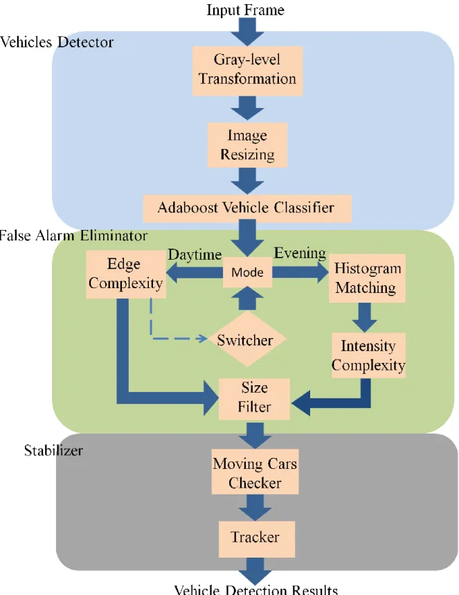
In this chapter, the structure of proposed system is defined. The system structure is composed of three stages: vehicle detector, false alarm eliminator and stabilizer. Section 3.1 demonstrates the diagram of whole system and shows key modules of each stage. Section 3.2 explains the heart of vehicle detector, namely AdaBoost vehicle classifier, including concept and details. Section 3.3 illustrates the process and methods of false alarm eliminator. Section 3.4 explains how the system stabilizes the detection results and also erases some false alarms.

3.1 System Overview

First of all, we transform the raw color image into a gray level image and the gray level image is downsized by a simple downsampling algorithm for acceleration reason. After resizing, the image is send to AdaBoost vehicle detector to perform detection. Here, the detector uses slicing window to detect vehicles and confirms the results by its cascaded structure. The outputs of vehicle detector stage are candidate regions (CRs) of vehicles and are also the inputs of false alarm eliminator stage. In the second stage, we firstly check the erasing mode, namely daytime or evening. For daytime case, Canny edge operator [23] is applied to each CR, and then the system examines the edge complexity to decide whether the CR is vehicle or not. For evening case, system firstly calculates the histogram of each CR and then uses the histogram to do histogram matching and intensity complexity checking to verify the result. Both daytime and evening cases, all the results have to be examined by size filter to filter out too big or too small CRs. The final step is stabilizer stage. In this stage, we use survival algorithm to further ensure the CRs are vehicles and stabilize the detection results.

The diagram of whole system is shown in Figure 3-1.

3.2 Vehicle Detection using AdaBoost

This sub-system is the foundation of entire system, as mentioned in section 2.1, most research efforts have focused on feature extraction and classification by learning or statistical models. The most important issue in object detection is selecting a suitable set of features which can soundly represent the implicit invariant of interested objects. An intuitive method is to focus on the common components of interested objects. For example, contour, color, symmetry, texture and etc. are commonly use perceptual features. These features can be used alone or cooperatively to find interested objects in the searching area. Although these features can be easily implemented, they also have several limitations. One of the limitations is that these features are based on human’s perception and the physical nature of human’s perception is usually not reliable enough for computer vision. What’s more, how to choose a suitable set of features, no matter using single feature or combining features, is also a very difficult problem. Manually choosing is time consuming and inefficient. Therefore, the efforts of feature extraction have focused on statistical and machine learning area.

AdaBoost algorithm proposed by Y. Freund et al. [21] is one of machine learning techniques and has been widely used for pattern recognition. AdaBoost algorithm combines weak classifiers into one strong classifier by weighted voting mechanism, and it also showed high performance in various fields. P. Viola et al [24] used AdaBoost algorithm to built a pedestrian detector, which has progressively complex rejecting rules. In [19], AdaBoost algorithm is originally applied to face detection and yields the best performance comparable to previous researches. Like original idea, we want to use several features to describe a vehicle and use these features to detect vehicles. Therefore, we use Haar-like features, which will be introduced in section 3.2.1, to describe vehicle and use AdaBoost algorithm, which will be explained in details in section 3.2.3, to select useful Haar-like features and combine them into a strong classifier.

Our goal of this stage, namely AdaBoost vehicle detector, is to build a high detection rate vehicle classifier. In other words, we used detection rate as prime criterion to decode whether the performance of detector is good enough or not. The false alarm rate is treated as reference information about the detector and left to false alarm eliminator and stabilizer to deal with. We called this kind of training as non-converging training, which will be explained in section 3.2.5. The entire system is also designed and built under this concept.

3.2.1 Haar-like Features (Rectangle Features)

Haar basis functions (Haar-like features) used by Papageorgiou et al. [25] provide information about the grey-level intensity distribution of two or more adjacent regions in an image and is extended by Rainer Lienhart et al. [26]. Figure 3-2 shows the set of Haar-like features, including original and extended features. The output of a Haar-like feature on a certain region of gray-level image is the sum of all pixels intensity in the black region being subtracted from the sum of all pixels intensity in the white region. The sums of black and white region are normalized by a coefficient in case of square measures of white and black regions are different. In order to reduce computation time for the filters, P. Viola et al. [19] introduced the integral image which is an intermediate representation for a input image. The concept of integral image is illustrated in Figure 3-3(a), the value of the integral image at point (x, y) is the sum of all the pixels above and to the left. In Figure 3-3(b), the sum of the pixels within rectangle D can be computed with four array references. The value of the integral image at location 1 is the sum of the pixels in rectangle A. The value at location 2 is A + B, at location 3 is A + C, and at location 4 is A + B + C + D. The sum within D can be computed as 4 + 1 − (2 + 3). Utilizing integral images, sum of a rectangular region can be calculated by using only four references in the integral image. As a result, the difference of

image, eight in the case of the three-rectangle Haar-like features and nine for four-rectangle Haar-like features.

Every Haar-like feature j is defined as f( j ) = (rj, wj, hj, xj, yj), where rj is the type of

Haar feature, wj and hj are width and height of the Haar feature and (xj, yj) is its position in the

window. valuesubtracted  f( j), is the weighted sum of the pixels in white rectangles subtracted from those of dark rectangles.

Figure 3-2 The Haar features [26]

3.2.2 Weak Classifier

A weak classifier h(x, f, p, θ) consists of a Haar-like feature f (defined in 3.2.1), a threshold (θ) and a polarity (p) indicating the direction of the inequality in Equation 3-1.

     otherwise p x pf if p f x h 0 ) ( 1 ) , , , (   (3-1)

here x is a 22x18 sub-window of an image. For each feature j, AdaBoost algorithm is applied to decide an optimal threshold θj for which the classification error on training database

(containing positive and negative samples) is minimized. The process of threshold selection for weak classifier is a brute force method. We can think of threshold of weak classifier as a line that separate the positive sample from negative sample. The AdaBoost algorithm examines every separating threshold to find out the optimal threshold. The threshold seleting process is illustrated in Figure 3-4. By selecting the optimal threshold, the blue points (positive samples) and red points (negative samples) can be separated with a lowest classification error. Because one weak classifier has only one threshold, its separating ability is limited and that is why this kind of classifier being called weak classifier.

3.2.3 AdaBoost Algorithm

In literature, some methods are commonly used for features selection. For example, Principal Component Analysis (PCA) used in [14, 17, 18], Independent Component Analysis (ICA) used in [18] and so forth. Compared with above methods, AdaBoost algorithm has shown its capability to improve the performance of not only features selection but also detection rate.

In the beginning, we have to prepare a feature set originated from the permutation of Haar-like feature types, scales and positions. This features set is many times greater than the number of pixels in the input image. Even though each Haar-like feature can be computed very efficiently by integral image, computing the complete set is still extremely time consuming and costly. AdaBoost algorithm uses this feature sets to generate weak classifiers and finds precise hypotheses of vehicle by iteratively combining weak classifiers which, in general, have moderate precision into a strong classifier defined in Equation 3-2.

    _ 





where h and C are the weak and strong classifiers respectively, and α is a weight coefficient for each h.

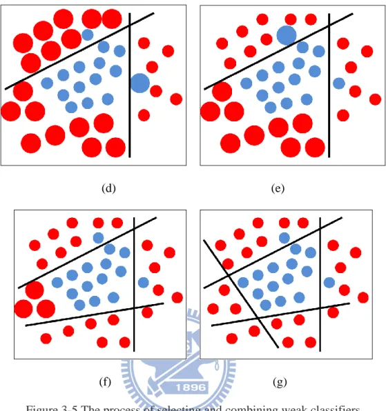
Considering a 2D feature space is full of positive and negative training samples. At first, AdaBoost algorithm chose a weak classifier with the highest accuracy in current training round to split the training samples by its optimal threshold. As shown in Figure 3-5(a), samples misclassified by previous weak learner are given more attention before adding next weak classifier at next round. By increasing weights, the training process will focus on these difficult samples, which cannot be correctly separated by single weak classifier. The idea of

how AdaBoost algorithm selects and combines weak classifiers into a strong classifier is

(positive samples) in right side of the black line and red points (negative samples) in left side of the black line are emphasized in the next round as Figure 3-5(c). Similarly, the misclassified blue points in left side of the second black line and red points in right side are emphasized in the next round, as shown in Figure 3-5(d) and Figure 3-5(e). Finally, the strong classifier is formed with a linear combination of weak classifiers shown in Figure 3-5(g), and the boosting algorithm for selecting a set of weak classifiers to compose a strong classifier is shown in Table 3-1.

(a)

(d) (e)

(f) (g)

Table 3-1 The boosting algorithm for selecting and combining weak classifiers[29]

3.2.4 Cascaded Classifier

A cascaded classifier is a linear combination of strong classifiers, and strong classifier is composed of at least one weak classifier. P. Viola et al [19] also proposed a cascading

algorithm of AdaBoost described in Table 3-2. At each stage, if an input extracted by the

searching window is classified as vehicle, it is allowed to enter the next stage; otherwise, the

T hypotheses are constructed and each using a single feature. The final hypothesis is a weighted linear combination of the T hypotheses where the weights are inversely proportional to the training errors.

• Given example images (x1, y1), . . . , (xn, yn) where yi = 0, 1 for negative

and positive examples respectively.

• Initialize weights w i m 2l 1 , 2 1 , 1 

for yi = 0, 1 respectively, where m and l

are the number of negatives and positives respectively. • For t = 1, . . . , T :

– Normalize the weights,



– Select the best weak classifier with respect to the weighted error



– Define ht(x) = h(x, ft, pt, θt) where ft ,pt ,and θt are the minimizers of

εt.

– Update the weights:

i e t i t i t w w_1,  _,1

where ei = 0 if example xi is classified correctly, ei = 1 otherwise,

and t t t      1

• The final strong classifier is:

    _ 





can be labeled as vehicle; otherwise it is rejected by particular stage even if it enters the last stage. Figure 3-6 demonstrates the schema of cascaded classifier.

Table 3-2 The training algorithm for building a cascaded detector[29]

Figure 3-6 Structure of cascaded classifier.

• User selects values for f, the maximum acceptable false positive rate per layer and d, the minimum acceptable detection rate per layer.

• User selects target overall false positive rate, Ftarget.

• P = set of positive examples • N = set of negative examples • F0 = 1.0; D0 = 1.0 • i = 0 • while Fi > Ftarget – i ← i + 1 – ni = 0; Fi = Fi-1 – while Fi > f × Fi-1 * ni ← ni + 1

* Use P and N to train a classifier with ni features using AdaBoost

* Evaluate current cascaded classifier on validation set to determine

Fi and Di.

* Decrease threshold for the ith classifier until the current cascaded

classifier has a detection rate of at least d × Di-1 (this also affects

Fi)

– N ← 0

– If Fi > Ftarget then evaluate the current cascaded detector on the set of

3.2.5 Non-Converging Training

As far as machine learning is concerned, training samples play a very important role in the training process. There are many factors of training samples can affect the final performance of classifier. For example, the amount of training samples, the complexity of content in the training image and etc. Commonly, positive training samples contain similar images of interested object. For instance, the positive training samples have similarity in the phase of interested object, lighting condition, contour and so forth. When collecting positive training samples, it is important to make the difference between each sample as low as possible. In the other words, the main purpose of positive training samples is to provide training algorithm the common features of interested object. On the other hand, negative training sample is everything except interested object. In this study, the interested object is vehicles and we focus on the front phase of vehicles.

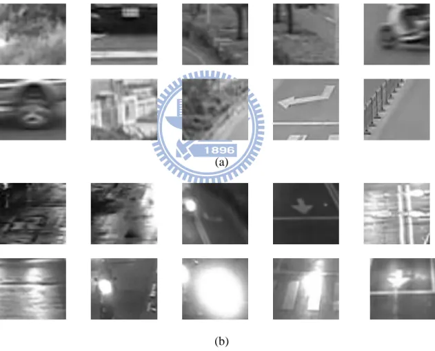
Different from the normal concept of preparing training samples, we collected not only similar samples but also dissimilar samples. More precisely, we collected frontal-viewed image of vehicles for positive samples and the others for negative samples both from daytime and evening. The samples have quite difference in lighting condition and have different features. Figure 3-7 is some positive samples we collected, including daytime and evening and Figure 3-8 is some samples of negative samples.

(b)

Figure 3-7 Some positive training samples of (a) Daytime (b) Evening

(a) (b)

Figure 3-8 Some negative training samples of (a) Daytime (b) Evening

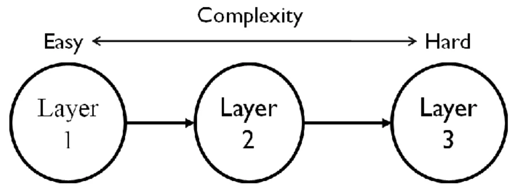
Generally, the complexity of training samples will affect the convergence of training process. That means if the content of training samples is too difficult, the training process of

AdaBoost algorithm would not finish, namely non-converging. According to algorithm described in Table 3-1, AdaBoost algorithm will pay more attention to the hard samples, which is difficult to classify by single weak classifier. What’s more, by algorithm described in Table 3-2, AdaBoost will build progressively complex decision rules in order to deal with hard samples when the training process is going on, illustrated by Figure 3-9. As you can see in Table 3-2, the outer while loop will continue until the Fi is small than Ftarget. Therefore, if the training samples are too complex to classify, the training process will never stop. Besides, the performance criterion of cascading algorithm is false alarm rate. In order to fit this criterion, the training process will try to decrease false alarm and the detection rate will decrease simultaneously.

Figure 3-9 Progressively complex decision rules of AdaBoost vehicle detector

Because we increased the complexity of training samples, it is not realistic to expect the training process will converge. As the consequence, we use detection rate as prime criterion instead. By the algorithm described in Table 3.2, the more layers the classifier has, the more difficult the object is classified as a vehicle. Consequently, if we decrease the layer number of classifier, the chance that the object be classified as a vehicle is higher. Therefore, what we did here is to specify the training process will stop at particular layer number. It doesn’t matter that the training procedure is not converge yet, we just want the classifier can detect as

as assistant criterion. The statistical results will be presented in section 4.

3.3 False Alarm Eliminator

As mentioned in section 3.2, this stage of system is to handle the false alarms generated from previous stage, namely AdaBoost vehicle detector. The first priority of false alarm eliminator is to filter out false alarms as many as possible and affect detection rate as less as possible. When decreasing false alarm rate, as mentioned in section 3.2.5, the detection rate is affected simultaneously. Therefore, how to decrease false alarm rate and still keep detection rate as high as possible in the same time is the primary issue in this step. Additionally, the complexity of computation is also one of our concerns because we also want the system can be applied to real-time applications. As the results, we used less complex methods cooperating with properties of vehicles to filter out false alarms.

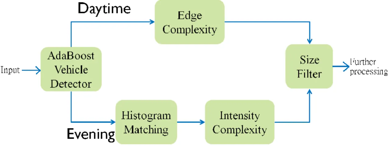
Because the system has to deal with the false alarms both from daytime and evening, the false alarm eliminator has two schemes for daytime and evening respectively. For daytime case, we use edge complexity, illustrated in section 3.3.1, to identify which candidate region (CR) generated from AdaBoost vehicle detector is vehicle and which CR is not. As for evening case, we use histogram matching and intensity complexity, explained in section 3.3.2, to filter out false alarms and retain vehicle objects. In the end, both for daytime and evening cases, the system will use size filter, introduced in section 3.3.3, to filter out too big or too small CRs. For automatic detection reason, we also proposed a switching algorithm, illustrated in section 3.3.4, to let the system decides which scheme to be used by itself. Figure 3-10 is the two schemes of false alarm eliminator.

Figure 3-10 Two schemes of false alarm eliminator

3.3.1 Edge Complexity

In the daytime, there are some features can be used to describe a vehicles. For examples, Luo-Wei Tsai et al [27] used color, edge and corner to identify vehicles in the static image

and A. Kuehnle et al [2] used the symmetry of edge as features of vehicles. In this study, we

do not consider using color as one of the features because the Haar-like features used in AdaBoost algorithm are operating on gray-level image. In the other words, the AdaBoost vehicle detector we trained uses only gray-level information. Further, we do not use corner to verify the results of AdaBoost vehicle detector. It is hard to discriminate vehicle objects from non-vehicle objects by using corner only, because there are too many objects have similar shape as vehicles. As the consequence, it is hard to eliminate the false alarms efficiently by using the number of corners on the objects or the position information of corners. In our false

alarm eliminator, we chose edge as the main feature and use edge complexity [28] to identity

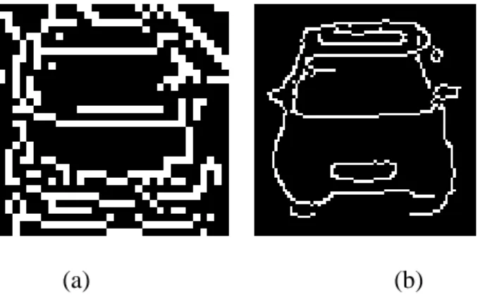
Figure 3-11 Some examples of edge image

First, we use Canny operator [23]to obtain the edge image of each CRs. Figure 3-11 is some edge image examples. After acquiring the edge image, we do not use the whole edge image to compute the edge complexity. Instead, we just utilize the bottom-half part of edge image. It is because that the top-half part of CR is more likely to contain background objects that will provide extra edge complexity and affect the accuracy. Therefore, we just look at the bottom-half part of CR and compute the edge complexity here by Equation 3-3. The other reason for just looking bottom-half part of CR is that the head of vehicles is usually in the bottom-half part of CR and the edge complexity here is discriminative if the CR is not vehicle object. Figure 3-12 is an example of bottom-half part of vehicle object.

where mc is the edge complexity, is the number of edge pixel and n is the number of pixel.

An CR is verified by Equation 3-4.

(3-4)

where and are empirical thresholds for the purpose of effective verification.

By using edge complexity of the bottom-half part, the system can filter out some false alarms, mostly the CRs which include the road, efficiently.

3.3.2 Histogram Matching and Intensity Complexity

Although the edge complexity can perform well in the daytime, its capability is decreasing as time approaches evening. The main reason is that vehicles will turn on their front lamps when the weather is going darker and we only use the bottom-half part of candidate region (CR), where the lamps locate, to compute edge complexity. Because of the light comes from the lamps, the edge complexity of vehicles drop off dramatically causing its discriminative ability being not suitable for evening case. In addition, the dark lighting condition makes the color, contour and edge of vehicle become ambiguous. On the other hand, the lighting lamps become the most obvious feature of vehicle in the evening. Consequently, we use the lighting lamps as the main feature instead and utilize them to filter out false alarms. Figure 3-13 is the example of edge image in the daytime and evening respectively.

There are two steps to identify the false alarms as illustrated in Figure 3-10. The system uses histogram matching to filter out the false alarms, mostly are ground images, and use intensity complexity to confirm the CRs being vehicle images or not. These two methods are constructed into cascaded structure inspired by AdaBoost algorithm. By cascaded structure, each step, namely histogram matching and intensity complexity, can deal with relative simple problem and filter out false alarms efficiently.

First, Figure 3-14 demonstrates two images, namely a false alarm image (ground image here) and a vehicle image, and their histogram image respectively.

(a) (b)

(c) (d)

Figure 3-14 (a) vehicle image (b) ground image (c) histogram of (a) (d) histogram of (b)

different from ground’s. Unfortunately, the light come from lamps is also projecting on the road causing the histogram of ground can sometimes be similar with the histogram of vehicle. Besides, the intensity of vehicle body can also be confusing because other vehicle’s lamps might project on the other vehicle. In the other words, we cannot be sure that the histogram that we computed can represent the lamps. Therefore, we do not use the entire image to compute the histogram and the range of histogram is not typical 0~255.

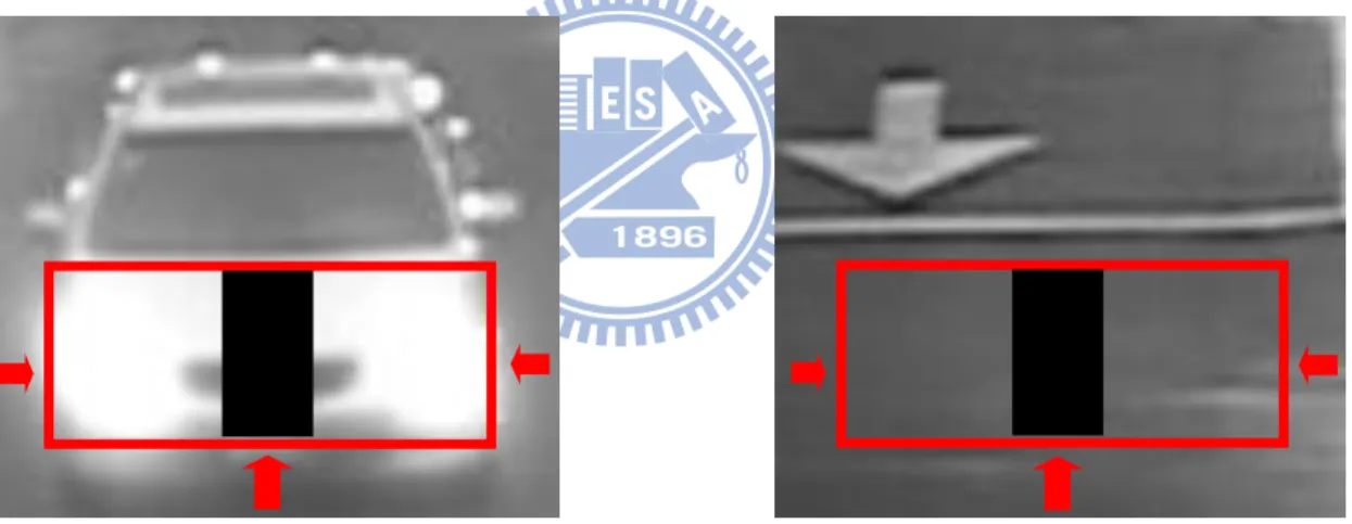
What we do here is similar to the idea of edge complexity. Because the lamps are usually locating at the bottom-half part of candidate region (CR) and they are approximately symmetric to the middle vertical line of CR, we utilize these properties to select sub-region to computer histogram. Figure 3-15 illustrates the sub-region we chose.

Figure 3-15 Sub-region to compute histogram

It is important that the histogram we computed is almost generated from the intensity of lamps. As Figure 3-15, we first look at bottom-half part of CR and reduce the range of left, right and button boundary. The purpose of reducing the range of sub-region is to decrease the impact of background image because the CRs always contain some background image. By reducing the range of sub-region, we can more precisely locate at the position of lamps.

sub-region to zero. This is because the lamps are approximately symmetric to the middle vertical line of CR. Therefore, we assume the pixels around the middle vertical line and within the sub-region cannot represent the lamps and we do not want to include these pixels. Thirdly, we only include the pixel whose intensity is high than 110 when computing the histogram. By limiting the range of intensity, the difference between the false alarms and vehicle objects can be enlarged. Figure 3-16 illustrates the result of our method.

(a) (b)

(c) (d)

Figure 3-16 (a) Vehicle image (b) Ground image (c) histogram of (a) (d) histogram of (b)

After computing the histogram of each CR, we compare histograms with our two target histograms, which are selected from our training samples and tested by Equation 3-5.

(3-5)

where ρ is the correlation coefficient, X and Y are two random variables, E is the expect value operator, Cov means covariance and σ is standard deviations. The whole procedure of histogram matching is illustrated in Figure 3-17.

Figure 3-17 Procedure of histogram matching

As Figure 3-17, the structure of histogram matching is also cascaded structure. It is unrealistic to expect one histogram can handle most false alarms. Therefore we use cascaded structure to filter out false alarms as many as possible. After all, we still has next step, namely intensity complexity, and stabilizer to erase false alarms.

The next step is intensity complexity which is inspired by edge complexity and further utilizes the histogram information. In the histogram matching step, we already have the histogram of each CR and also the amount of pixels whose intensity range from 110 to 255.

confirms the CR is vehicle objects. The intensity complexity is computed by Equation 3-6.

where is the amount of pixels whose intensity is between 155 and 255 and n is the

number of pixels of sub-region which used to compute the histogram in histogram matching step.

The purpose of intensity complexity is to examine the existence of lamps and further confirm the CR is vehicle object. The falsification is by Equation 3-7. The idea here is similar with edge complexity. In edge complexity step, we use the complexity to represent the head of vehicles. As for intensity complexity, we use the complexity to represent the lamps. As mentioned in histogram matching, we utilize not only the intensity of bright pixels come from lighting lamps but also the position of lamps. Therefore, we only select pixels whose intensity range from 155 to 255 and location is within the assumed area to compute intensity complexity.

(3-7)

where η is empirical threshold.

The system uses the light lamps, which are the most obvious feature of vehicles in the evening, to filter out the false alarms and remain the vehicles object instead of using edge complexity. This scheme let the system can operate in evening.

3.3.3 Size Filter

When we use video as our input, one vehicle will continuously show up at different positions and then disappear. What’s more, the vehicle has specific width at particular position. As the consequence, we can filter out unreasonable candidate region (CR) whose

width is too big or too small at its position by utilizing this property. Figure 3-18 illustrates the concept and Equation 3-8 and Equation 3-9 are the computing formulas.

Figure 3-18 Width of vehicle at different position

(3-8)

(3-9)

Besides using Equation 3-8 and Equation 3-9, we also set a tolerance rage for acceptable width and the final filtering rule is Equation 3-10.

(3-10)

where ε is the empirical threshold for efficient falsification.

decide using what feature to represent the passing time. As mentioned at section 3.3.2, we use histogram matching and intensity complexity to filter out false alarms instead of using edge complexity because the average value of CR’s edge complexity will decrease when the time approaches evening. Therefore, we use nothing but edge complexity to detect the changing of time. Figure 3-19 is the flow chart of switcher.

The system will operate the switching every 5 frame. When the system is going to compute the average edge complexity of CRs, we expect that there are enough CRs. This is because the result is not precise enough when there are too less CRs. For example, if there is only one CR, which might means there is only one vehicle in the scene and use edge complexity of only one CR to decide the average value is increasing or decreasing, it is not suitable. After all, we want to observe the trend of edge complexity to help us decide which scheme to use. Therefore, we have to check if there are enough CRs. If there are enough CRs, we compare the average value of CR’s edge complexity with the threshold by Equation 3-11 and record the result. We still have to record enough result in order to analysis the trend of edge complexity.

(3-11)

where is the button threshold of edge complexity, 1 means increasing and -1 means

decreasing.

After collecting enough data, we compute the number of 1 and -1 respectively, if the number of 1 is bigger than -1’s, we consider that the trend is increasing, otherwise is decreasing. Still, we do not judge only by one decision. The system won’t change the scheme until there are enough trend decisions. In our system, we set the threshold to 3 decisions. It means that if the switcher has 3 decreasing decision and current scheme is daytime, for example, the switcher will change the scheme to evening. We combine the two schemes by the algorithm explained above and let the whole system can operate both at daytime and evening with automatic detection functionality.

3.4 Stabilizer

The stabilizer is usable when the input is video and it is the final stage of our system. There are two missions for this stage. One is to stabilize the detection results and the other is to filter out the false alarm. When the input is the video, the system will operate on every frame. Sometimes, the same vehicle is detected in current frame but is missing in next frame and then is detected again. Even though there are no significant differences between continuous frames, the missing situation will happen. This is because no matter the AdaBoost vehicle classifier or the false alarm eliminator, all of them use threshold to detect and falsify. Therefore, even if the value is higher or less than threshold by 0.001, the result is completely different. As the consequence, the detection results might have the twinkling detection rectangle and that is the problem we want to solve.

There are two steps of this stage, namely stabilizer. One is confirming step which is the final method to erase false alarms and the other is tracking step which is used to solve twinkling rectangle. The former will be introduced in section 3.4.1 and the latter will be explained in section 3.4.2.

3.4.1 Confirming Step

The final result we want to present is the detection rectangles which contain vehicles in the current scene. Therefore, we have to make sure the content of detection rectangles is vehicles and that is also the reason why we develop false alarm eliminator. But the false alarm eliminator has its limitation, namely it sometime cannot filter out all the false alarms because the threshold method as mentioned at section 3.4. As the consequence, we use survival algorithm, which utilizes the fact that a vehicle will show up in the scene continuously when the input is video, to make sure the detection rectangles is not false alarms. Figure 3-20 is the flow chart of confirming step.

Figure 3-20 The flow chart of confirming step

After the AdaBoost vehicle detector generates the candidate regions (CRs) and these CRs are examined by false alarm eliminator, we check our survival list whether already has the same CR or not. We use the distance of left-up corner to distinguish it. Figure 3-21 illustrates the idea.

Figure 3-21 Two detection rectangles of the same vehicle

For each CR, we compute the distance between two left-up corners with every detection rectangle in the survival list. If there is a distance less than maximum acceptable distance and is also the minimum distance among all the rectangles in the survival list, we think of the CR and the closest detection rectangle in the survival list are the same and we increase its hitting number, which is explained in next paragraph. Otherwise, we add current CR into the survival list.

The hitting number is the implementation of the survival concept. As mentioned at section 3.4, a vehicle will show up in the scene continuously and then disappear. What’s more, we operate the detection step at every frame. Therefore, a vehicle will be detected more than once before disappearing. We accumulate the number of detection, namely the hitting number, to distinguish the vehicles from the false alarms. If a CR is detected more than hitting number threshold within specific frame interval, the CR is treated as vehicle object. By applying this survival concept, we can further erase the false alarms which the false alarm eliminator cannot handle and confirm the CR is actually the vehicle object.

3.4.2 Tracking Step

rectangle no matter that it is missed by AdaBoost vehicle detector or filtered out by false alarm eliminator. As long as the detection rectangle is confirmed as vehicle object, the detection rectangle will be drew until the vehicle is out of sight. By this step, we can avoid twinkling detection rectangle. If the same detection rectangle is generated by AdaBoost vehicle detector and pass the false alarm eliminator again, we update the position information and size of this detection rectangle and then draw the detection rectangle. Otherwise, we draw the detection rectangle by the information stored in survival list and use simple tracking algorithm to update the position. Figure 3-22 is the diagram of this step.

Figure 3-22 Diagram of tracking step

detection iteration, namely every frame finishes, we examine the survival condition of every detection rectangle in the survival list. If the detection rectangle is out of sight or it does not meet the survival criterion, the detection rectangle should be deleted.

Chapter 4

Experimental Results

The vehicle detection system is implemented on a PC system. The CPU and RAM of the PC is Intel Core 2 Duo @ 2.9G and 2GB RAM respectively. The integrated development environment is Microsoft Visual Studio 2008 on Windows XP OS. The inputs are video files (uncompressed AVI) or images (PPM format). These inputs were captured with a DV at traffic intersection or testing samples which were used by other research.

Section 4.1 illustrates the training process of AdaBoost, including the training dataset and the comparison of non-converging training at different layer number. Section 4.2 shows the results of detection in static image with the comparison of other researches. The testing images are obtained from a public testing database – MIT CBCL car database 1999. Section 4.3 demonstrates the experimental results of switcher. Section 4.4 illustrates the experimental results of detecting vehicles in videos.

4.1 AdaBoost Training

We collected our training data by manually extracting samples from videos. There are 3431 positive samples and 11133 negative samples. Both the positive samples and negative samples contain daytime and evening samples. All the training samples are transformed into gray-level image. Because the samples are collected manually, they do not have the same size. Therefore we normalized the sample to 22 x 18. The weak classifiers used here are the permutation of the type, position and scale of 15 Haar-like features. Figure 4-1 demonstrates some samples of positive and negative samples and Figure 4-2 is the flow chart of the training

(a-1)

(a-2)

(a) Positive samples of (a-1) Daytime (a-2) Evening

(b-1)

(b-2)

(b) Negative samples of (b-1) Daytime (b-2) Evening Figure 4-1 Some samples of training samples

Figure 4-2 Flow chart of AdaBoost training process

As mentioned at section 3.2.5, we used non-converging training method to train our AdaBoost vehicle detector. Table 4-1 is the statistical result of different layer number. The testing data is MIT CBCL car database. The criteria of performance measurement are defined in Equation 4-1 and 4-2 [18].

(4-1)

Table 4-1 Comparison between different AdaBoost vehicle detector # of layers 14 13 11 10 9 8 Number of weak classifiers 592 477 318 263 210 179 Detection Rate 61.18% 68.63% 85.71% 94.41% 98.14% 98.76% False Alarm Rate 0% 0.00008% 0.0008% 0.0014% 0.003% 0.0058%

Obviously, the less number of the layer is, the higher the detection rate is. It is because when we decreased the number of the layer, we actually decreased the complexity of AdaBoost decision rules. Look at the last two columns, namely AdaBoost vehicle detector with 9 layers and 8 layers. Although, both of these two AdaBoost vehicle detector’s detection rate are higher enough, they can be distinguish from each other by false alarm rate. When we decrease the layer number from 9 to 8, the detection rate increases 0.62%, but the false alarm rate also increases 0.0028%. The price of increasing only 0.62% detection rate is too high and it also means that we have to deal with much more false alarms. Therefore, in this study, the layer number of AdaBoost vehicle detector is 9.

4.2 Results of Detecting Vehicles in Static Image

to the size 128x128 and aligned so that the car was in the center of the image. There are few researches that provided the experimental result of public frontal-viewed car database. So far, R. Wang et al. [18] provided their experimental result of MIT CBCL car database. We also implemented the method proposed in J.F. Lee [29]. Therefore, we compared the experimental result of [18] and [29] with that of the proposed system and the comparison results are presented in Table 4-2 and some detection results are presented in Figure 4-3. Because the MIT CBCL database consists of daytime image, we only use daytime scheme without size filter, namely AdaBoost + edge complexity, to test the performance. The criteria of performance measurement are also Equation 4-1 and 4-2.

Table 4-2 Performance comparison of MIT CBCL

PCA + ICA AdaBoost + PDBNN Proposed System

Detection Rate 95% 91.93% 96.27%

False Alarm Rate 0.002% 0.0031% 0.0015%

Figure 4-3 Some detection results of MIT CBCL car database

4.3 Results of Switcher

First, we show that why we have to design a switching algorithm, Figure 4-4 is the statistic charts of two false alarm eliminating schemes respectively. The purple line labeled with Edge is the daytime scheme and the blue line labeled with Hist is the evening scheme. The video sequence is in the time interval from daytime to evening.

Figure 4-4 Statistic charts of two false alarm eliminating schemes

As illustrated in Figure 4-4, the detection capability of daytime scheme is falling down when time approached evening. Although the evening scheme has high detection rate in the daytime but its false alarm rate is too high. Figure 4-4 explains why we need two schemes to handle false alarms in different time interval and why we have switcher to combine these two schemes. The Figure 4-5 demonstrates the result after integrating the switching algorithm.

Figure 4-5 Statistic chart of integrating switcher

4.4 Results of Detecting Vehicles in Video

In this section, the experimental results of detecting vehicles in videos are demonstrated. We compared the result with J.F. Lee [29], namely AdaBoost + Probabilistic Decision-Based Neural Network (PDBNN) and method which used Gaussian Mixture Model (GMM)[30][31] to establish background image. The testing videos are composed of daytime and evening traffic video and different scenes. Table 4-3 to Table 4-7 are the statistic results of testing videos. We also present comparison of the frame per second (FPS). Table 4-3 to Table 4-5 are comparison result of daytime testing videos and Table 4-6 to Table 4-7 are the comparison result of evening testing videos. The detection rate and false alarm rate are computed by Equation 4-3 and Equation 4-4 respectively.

(4-3)

Table 4-3 Performance comparison of video at scene 1 (Daytime)

Place Method Detected

vehicles

False alarms FPS Total

vehicles 台中市 大墩路 GMM 110 ( 82.09% ) 7 ( 5.98% ) 20.745 134 AdaBoost + PDBNN 131 ( 97.76% ) 2 ( 1.5% ) 7.445 Proposed system 133 ( 99.25% ) 2 ( 1.48% ) 17.265

Table 4-4 Performance comparison of video at scene 2 (Daytime)

Place Method Detected

vehicles

False alarms FPS Total

vehicles 新竹市 東光路 GMM 121 ( 72.46% ) 57 ( 32.02% ) 21.19 167 AdaBoost + PDBNN 153 ( 91.62% ) 3 ( 1.92% ) 4.52 Proposed system 163 ( 97.6% ) 8 ( 4.54% ) 16.35

Table 4-5 Performance comparison of video at scene 3 (Daytime)

Place Method Detected

vehicles

False alarms FPS Total

vehicles 新竹市 光復路 GMM 103 ( 81.75% ) 110 ( 51.64% ) 21.28 126 AdaBoost + PDBNN 41 ( 32.54% ) 5 ( 10.87% ) 6.856 Proposed system 124 ( 98.41% ) 2 ( 1.59% ) 18.417

Table 4-6 Performance comparison of video at scene 1 (Evening)

Place Method Detected

vehicles

False alarms FPS Total

vehicles 台中市 大墩路 GMM 139 ( 79.89% ) 87 ( 38.5% ) 21.295 174 AdaBoost + PDBNN 148 ( 85.06% ) 2 ( 1.14% ) 8.295 Proposed system 173 ( 99.43% ) 8 ( 4.42% ) 17.167

Table 4-7 Performance comparison of video at scene 3 (Evening)

Place Method Detected

vehicles

False alarms FPS Total

vehicles 新竹市 光復路 GMM 283 ( 87.35% ) 265 ( 48.36% ) 21.605 324 AdaBoost + PDBNN 180 ( 55.56% ) 45 ( 19.74% ) 5.37 Proposed system 310 ( 95.68% ) 10 ( 3.125% ) 19.466

In the daytime, both method in [29] and our proposed system perform well. As for GMM, because the scenes we used have heavy traffic and contain vehicles and motorcycles in the same time, it is hard for GMM method to segment vehicle will and distinguish motorcycle from vehicle. In the evening, our system is better than [29] and [30][31] with higher detection rate and acceptable false alarm rate. The detection rate of [29] decreased when time approach evening because the edge of vehicle become ambiguous. For [30][31], problem generated by motorcycles still exit. What’s more, the light come from lamps of vehicle generated more trouble. As for operation speed, our proposed system is also faster than [29] and near [30][31].

As illustrated in Table 4-3 to Table 4-7, the result is identical to our objective, namely can be applied to real-time application. Figure 4-6 is some capture pictures of detection result. The red rectangle is the result of proposed system and green rectangle is the result of [29] and yellow rectangle is the result of GMM.

(a)

(b)

(c)

(d)