資訊透明度對一籃子信用違約之影響

國 立 交 通 大 學

財 務 金 融 所

碩 士 論 文

資訊透明度對一籃子信用違約之影響

How Does the Transparency of Information Affect the Spreads

of Basket Default Swap？

研 究 生：張曉茹

指導教授：郭家豪 博士

資訊透明度對一籃子信用違約之影響

How Does the Transparency of Information Affect the Spreads

of Basket Default Swap？

研 究 生：張曉茹 Student：Hsiao-Ju Chang

指導教授：郭家豪 博士 Advisor：Jia-Hau Guo

國立交通大學

財務金融研究所碩士班

碩士論文

A Thesis

Submitted to Graduate Institute of Finance National Chiao Tung University in partial Fulfillment of the Requirements

for the Degree of Master of Science

in Finance May 2010

Hsinchu, Taiwan, Republic of China

i

資訊透明度對一籃子信用違約之影響

研究生：張曉茹 指導教授：郭家豪 博士

國立交通大學財務金融研究所碩士班

2010年5月

摘要

這篇論文是在首達時間的結構模型下著重於資訊透明度是如何影響

一籃子信用違約的交換利差。另外，同時我們也應用一因子高斯聯結

相依函數去衡量標的資產之間的違約相關性，使用蒙地卡羅模擬方法

後而得到的數值結果說明了：當標的資產的資訊愈透明時，會導致一

籃子信用違約的交換利差愈低，尤其是資產第一次發生破產的一籃子

信用違約交換上。

關鍵字：不完全資訊；高斯聯結相依函數；一籃子信用違約；透明度。

ii

How Does the Transparency of Information Affect the Spreads of Basket

Default Swap？

Student : Hsiao-Ju Chang Advisor : Dr. Jia-Hau Guo

Institute of Finance

National Chiao Tung University

ABSTRACT

This paper emphasizes on how the transparency of information influences the credit spread of basket default swap with a first passage time model. In addition, one factor Gaussian copula model is used to measure the default correlation between reference entities. Numerical results show that the more transparent the information is, the less the credit spread of basket default swaps is, especially for the first to default basket default swap.

Keywords: imperfect information; Gaussian copula; Basket default swap; transparency.

iii

Content

Chinese Abstract ... i English Abstract ... ii Content ... iii List of Figures ... iv 1. Introduction ... 1

2. The Basic Model ... 3

3. Default Probability with Default Correlations ... 8

4. Default Swap Spread of BDS ... 11

5. Numerical Results ... 13

iv

List of Figures

Figure 1. Credit default swaps ... 18

Figure 2. The spread under each k when a varies ... 19

Figure 3. The spread under each correlation coefficient when k varies ... 20

1

1. Introduction

This paper analyses the term structures of credit risk and credit spreads in secondary markets for the corporate debt of firms that are not perfectly transparent to bond investors. One of the most important problems in credit risk research is: What constitutes the corporate bond spread? In fact, the information market is asymmetric, so different transparency level is bound to affect the degree of credit risk spreads determined. In order to understand how transparency will affect the degree of spread, we study the implications of transparency information for term structures of credit spreads on basket default swaps (BDS). A BDS is a default protection instrument written on a basket of N bonds. The protection buyer pays a specified rate on a specified notional principal A until the kth ( kN) bond in the basket defaults or the contract expires. If the kthdefault occurs before the contract expiration, the buyer is entitled either to exchange the bond issued by the kth defaulted entity for its face value or to receive a cash equivalent payment.

However, the framework of BDS is the same as credit default swap (CDS), in what is referred to as a basket credit swap there a number of reference entities. The reference entity is usually a company or sovereign government. A first-to-default CDS provides a payoff only when the first default occurs. A second-to-default CDS provides a payoff only when the second default occurs. More generally, a k

2

th-to-default CDS provides a payoff only when the kth default occurs. Payoffs are calculated in the same way as for a regular CDS. After the relevant default has occurred, there is a settlement. The swap then terminates and there are no further payments by either party.

Take the first to default in the basket for example. The protection seller sells protection on the whole basket, but once there is one default in the basket, the transaction is settled and closed. And for the protection buyer, assuming the probability of the second default in a basket is quite low, he or she actually buys protection for the entire basket but paying a price which is much lower than the sum of individual prices in the basket. A BDS is an instrument that shift risk from one party to another.

This paper focuses on the effect of information transparency on credits spreads with a structural model (pioneered by Merton (1974)). There are some assumptions in this paper as follows：The investors can’t observe the issuer's assets directly, and they receive imperfect accounting reports. The market is arbitrage-free and the recovery rate is an exogenous variable.

Without loss of generality, basket credit spreads are characterized in terms of accounting transparency. Gaussian copula was used in this paper to describe the default correlation and it was combined with one factor Gaussian copula model to

3

simplify our model. Finally, Monte-Carlo simulation plays an important role to help us to get the fair credit spread of BDS.

Our paper proceeds as follows： Section II provides a description of the basic model. Section III derives the default probability with default correlations. Section VI describes how to obtain the credit spread of BDS. Section V gives numerical results to show the effect of information transparency on the credit spread of BDS. Section VI concludes.

2. The Basic Model

There are two credit risk models being used to describing the default process. One is the structural model (company value model), which is inspired by Merton (1974).The structural model is based directly on the issuer’s ability or willingness to pay its liability and it is usually framed around a stochastic model of variation in assets relative to liabilities. The other is the reduced-form model, also called the intensity model, originated by Jarrow and Turnbull (1995). The reduced-form model assumes an exogenously specified process for the migration of default probabilities, calibrated to historical or current market data.The main difference between the structural model and the reduced-form model is that the former considers the default as a stochastic event and it follows an assumed stochastic process.

4

This paper is based on the information transparency model simulated by Duffie and Lando (2001), and we applied the model with one factor Gaussian copula for the BDS. The stochastic process V describing the stock of assets of our given firm is modeled as a geometric Brownian motion, which is defined, along with all other random variables, on a fixed probability space( , , ) F  . In particular, ( )

,

i

Z t i t

V e

whereZ t_i( )Z₀m t_i _iW for i_i, 1, 2,..,N, for a standard Brownian motionW_i, a volatility parameter



_i> 0, and a drift parameter m_i  ( , )which determines the expected asset growth rate 1 2

, 0

log[ ( / )] / 2

i t E Vi t V mi i

 _  _{ } _{. All agents in our}

model are risk-neutral, and discount cash flows at a fixed market interest rate r. We will use the one factor Gaussian copula to define the correlation between W and _i Wj.

Then we try to find out that how the credit spread of BDS on the structural model varies with different transparency.

First, we turn to ask that how the secondary-market assesses the firm's credit risk and values its bonds. After issuance, bond investors are not kept fully informed of the status of the firms. While they do understand that optimizing equity owners will force liquidation when assets level fall to some sufficiently low boundary V_B > 0, and bond investors cannot observe the asset process V directly. Instead, they receive imperfect information at selected times t t₁, ,...,₂ t with _T t_i t_i1 .

5

report of assets, given by Vˆ_{i t,} , where log Vˆ_{i t,} and log V_{i t,} are joint normal. Specifically, we suppose thatY_{i t,} logVˆ_{i t,} Z t_i( )U t_i( ), where U t is normally _i( ) distributed and independent of Z t . (The independence assumption is without loss _i( ) of generality, given joint normality.) Also observed at each t[0, ) is whether the equity owners have liquidated the firm. That is, the information filtration (H ) _t

available to the secondary market is defined by ( H_t ) =

1 { }

({ ( ),..., ( ),1Y t Y tT s : 0 s t}),

 for the largest N such thatt_T t, where  (V_B). For simplicity, we suppose that equity is not traded on the public market, and that equity owner-managers are precluded, say by insider-trading regulation, from trading in public debt markets. This allows us to maintain the simple model (H ) for _t

the information reaching the secondary bond market, and avoiding a complex rational-expectations equilibrium problem with asymmetric information.

Our main objective for the remainder of this sub-section is to compute the conditional distribution of Vi t, given (H ). We will begin with the simple case of t

having observed a single noisy observation at time tt₁ .

We will need, as an intermediate calculation, the probability ( , ,z x₀  t) , conditional on Z starting at some given level z at time 0 and ending at some level ₀ x at a given timet, that min{Z_s: 0  s t} 0. As indicated by our notation, this probability does not depend on the drift parameter m , and depends on the variance

6

parameter 2

and time t only through the term k t _{. From the density of the}

first-passage time recorded in Chapter 1 of Harrison (1985), and from Bayes’ Rule, one obtains after some simplification that

2 2 ( , , )z x k 1 exp zx k    _ _   (1)

Next, z₀ Z₀ was fixed, we calculate the density b( | Yi t,,z t0, ) of Zi t, ,

“killed” at  inf{ :t Zi t, v} , conditional on the observation (Yi t, Zi t, Ui t, ). That

is, by using the conventional informal notation,

b x Y( | i t, , 0z , )t d x  Pi( t a n d ,i tZ d x Y,i t| ) , . (2) x v

Using the definition of  and Bayes' Rule,

0 , , 0 , ( , , ) ( ) ( ) ( | , , ) , ( ) i U i t Z i t Y i t z v x v t Y x x b x Y z t Y          (3) where i U

 denotes the density of U_{i t,} , and likewise for i Z  and i Y  .

These densities are normal densities, with meansE U( i t_, )ui,E Z( i t,)m ti z0,

and E Y( _{i t,} )m t_i  z₀ u_i , along with respective variances 2 , var(Ui t)ai , 2 , var(Zi t)it, and 2 2 ,

var(Yi t)ai it. The standard deviation ai of Ui t, may be

thought of as a measure of the degree of accounting noise. We have

P(i t Y| ,i t) v b z Y( |,i t ,0z , )t d z



 

_

. (4) Finally, we compute the density g( | Yi t_,,z t₀, )of Zi t, , conditional on the noisy

7 Rule, 0 0 , 0 ( | , , ) ( | , , ) ( | _{i t}, , ) v b x y z t g x y z t b z Y z t dz  



. (5) Letting y  y v u x, x v,andz z₀ v, a calculation of the integral in (5) leaves us with 0 ( , , ) 0 0 2 0 2 2 1 1 2 2 3 3 0 0 0 0 2 1 exp ( | , , ) , exp exp 4 2 4 2 J y x z z x e t g x y z t     _   _        _      _{ }                    _{ }   _{ }   _{ }   _{ }      (6)

where  is the standard-normal cumulative distribution function, and

2 2 0 0 2 2 ( ) ( ) ( , , ) , 2 2 z mt x y x J y x z a  t             With 2 2 0 2 2 0 1 2 2 0 2 1 2 2 2 0 3 2 2 , 2 , 2 , ( ) 1 . 2 a t a t z mt y a t z t z mt y a t                       _  _       

Given survival to t, this gives us the conditional distribution of assets, because the conditional density of V_{i t,} at some level v is easily obtained from the conditional density of Z_{i t,} at log v .

8

3. Default Probability with Default Correlations

We also compute the H -conditional probability_t p t s( , ) _{of survival to some future}

time s > t. That is, p t s( , )= (P_i s H| _t). For t_i, we have









, 0 ( , ) 1 , ( | _{i t}, , ) v p t s 



  s t x v g x Y z t dx ₍₇₎ 2 2 ( , ) mx x mt x mt t x N e N t t             _{ } _{ }     (8)

where ( , )t x _{denotes the probability of first passage of a Brownian motion with}

drift m and volatility parameter  from an initial condition x > 0 to a level below 0 before time t, which is known explicitly [Harrison (1985)].

Since we set up our model on Basket default swap, we want to accurately price the default correlation among the asset of BDS, the joint probability distribution with multi-factor has to be used. For simplicity, the copula model is a good choice which we can make good use of.

By above, we can get the survival probability p t s( , ) . Then, the default probability is F t s( , ) 1 p t s( , ) ,

















, 0 , 0 0 ( , ) 1 ( , ) 1 1 , ( | , , ) 1 , ( | , , ) i t v v i t F t s p t s s t x v g x Y z t dx s t x v g x Y z t dx              





(9)

When t approaches 0, it represents the underlying assets don’t default till now

and level x is fixed, then the function becomesF s( )F(0, )s _.

9

constructed using a copula function. A copula is a multivariate joint distribution defined on the N-dimensional unit cube [0, 1]N such that every marginal distribution is uniform on the interval [0, 1].

Specifically,C:[0,1]N [0,1] is an N-dimensional copula (briefly, N-copula) if:

i.

C( )u 0,whenever u[0,1]N has at least one component equal to

0。

ii. C( )u u_i,whenever u[0,1]N has all the components equal to

1

except the

i th one, which is equal to u 。 _i

iii. C u( )is N-increasing, i.e., for each hyperrectangle B _iN₁[ ,x y_{i i}][0,1] ,N

1 ( ) { , } ( ) : ( 1) ( ) 0. n i i i N C x y V B C   



 z  z z

where the N( )z card k z{ | _k x_k}. V B_C( ) is a so-called C-volume of

B

For multivariate case, Sklar's theorem can be stated as follows. For every multivariate distribution function CGa( ,u u_{1 2},....,u_N)

 

 

 



1 1 1



1 , 2 ,..., N u u u        , let G u1( )1 H u( , 0,..., 0)1 and 2( )2 (0, 2,..., 0),..., N( N) (0, 0,..., N)

G u H u G u H u be the univariate marginal probability distribution functions. Then there exists a copula C such that

H u u( ₁, ₂, . . . ,_Nu  )C G u₁( ₁ ( ₂G u) , ₂ ( _N) , . . . ,G_N (10) u ( ) ) where C is an identified cumulative distribution function. Moreover, if marginal distributions G u₁( ),₁ G u₂( ),...,₂ G u_N( _N) are continuous, the copula function C is unique. Otherwise, the copula C is unique on the range of values of the marginal

10

distributions.

One example of a copula often used for modeling in finance is the Gaussian copula, which is associated with the multivariate normal random variables that display the correlation structure induced by linear dependence on a single normally distributed factor via Sklar's theorem.

Suppose the correlation coefficient between X and M is fixed, called it as, and doesn’t change by time, i.e.,  _{is a constant.}Let X be the random variable _i

such that

2

1 , 1, 2,3,...,

i i

X M    i N (11) where  Y , M and  are standard normal distributed random variable. Obviously, X is also a random variable of normal distribution and the correlation coefficient _, i j X X  between X and _i Xj is 2  .

This is the most common copula model used in pricing basket default swaps. It is also used by market participants as a convention to quote the BDS prices in terms of the correlation coefficients. With _ being the standard multivariate normal cumulative distribution function with correlation coefficient, the Gaussian copula function is



1 1 1



1 2 1 2 ( , ,..., ) ( ), ( ),..., ( ) , Ga N N C u u u   _  u  u  u (12) where u u₁, ₂,...,u_N[0,1]and

Φ

denotes the standard normal cumulative distribution

11

function.

4. Default Swap Spread of BDS

We suppose that there exists a BDS paying the swap rate annually in the end of the period, and pay date of bond interest is at t t t₁, , ...,_{2 3} t . Denote the basket default _T

spread as c, the principal asA, the recovery rate as q, and the discount rate as r. Let _k be the default time of kth entity, then  ₁ ₂₃..._N . The protection seller will pay the contingent payment A (1 q) when it defaults.

The protection buyer has to pay the basket default swap spread if it doesn’t default at t . Take first to default for instance, if _i t₄  ₁ t₅, the protection buyer will have to pay the premium payment _A _{(c e}rt1 _{c e}rt2 _{c e}rt3 _{c e}rt4_{), but he}

or she will also receive the contingent payment _A  _{(1 q) e}r1_{from the protection}

seller when the reference entity defaults. The former and the latter must be equal in deciding a fair default swap spread.

3

1 2 4 1

( rt rt rt rt ) (1 ) r

A c e  c e  c e  c e    A q e ₍₁₃₎ If we want to calculate the fair default swap spread in a risk-neutral world, the expected value of the contingent payment paid by the protection seller must be equal to the expected value of the premium payment paid by the protection buyer.

12 [ ] [ ] [ / ] [ ] E C o n t i n g e n t P a y m e n t E L c E P r e m i u m P a y m e n t m u l t i p l i e d b y t h e P r i c i p a lB c E   (14) where L is the contingent payment,

B is (the premium payment multiplied by the principal)/c. E[.] is the expected value.

By Gaussian copula, we can assume that

 







 





 



1 1 1

1 τ1 , 2 τ2 ,..., N τN

X   F X   F X   F using the correspondence of normal cumulative distribution function (CDF) to get the default time

1, 2, ...,3 N

    of the N underlying assets that _i F1



(X_i) ,



i1, 2,3,...,N, where the random variable X is defined in section III, and _i F is the default probability function. In evaluating the basket default swap spread by the Monte-Carlo simulation, if we take the number of simulation as F, and the contingent payment under the s th simulation is：

(1 ) r sk ( s ), 1, 2,...,

s k T

L    A q e I  t s F (15) where _ks is the default time of the kth defaulted entity of N at s th simulation. And I( ) is an Indicator Function.

And the sum of the premium payment at s th simulation multiplied by the principal is： 1 ( ), 1, 2,..., i T rt s s i k i cB cA e I t s F   



  (16) After the simulation of F times, the expected value of the contingent payment

13

paid by the protection seller is

1 1 F s s L F



 , and received 1 1 F s s c B F  



as the expected value of the premium payment multiplied by the principal before the kth entity defaults from the protection buyer.

Therefore, the fair basket default swap spread should be：

1 1 F s s F s s L c B   





(17) The following is the relationship amonga _{, k ,} and c with simulation 10000

F  paths .

5. Numerical Results

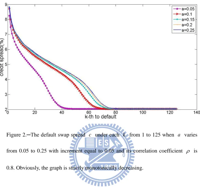
Our main result is in the Figure 2, it shows that the larger the k th to default is, the smaller the basket default swaps spread c is, it also shows that the bigger the volatility a (the lower transparency level) is, the bigger the basket default swaps spread c is. That is, volatility a and the basket default swaps spread c change in the same direction, but k th to default and the default swaps spread c change in opposite.

In addition, Figure 2 also shows that the differences of basket default swaps spreads c of different scales of volatility a gets fewer when a gets bigger, there seems existing a tendency. For example, let l be the difference between basket

14

default swap spread c_0.25 under a0.25 and basket default swap spread c_0.2

under a0.2, (that is, l =c_0.25-c .), m be the difference between _0.2 c_0.2 and basket default swap spread c_0.15 under a0.15 , (that is, m =c_0.2 -c_0.15 .), n be the difference between c_0.15 and basket default swaps spread c under_0.1 a0.1, (that is,

n =c_0.15-c .). We can have the conclusion of l < m < n . _0.1

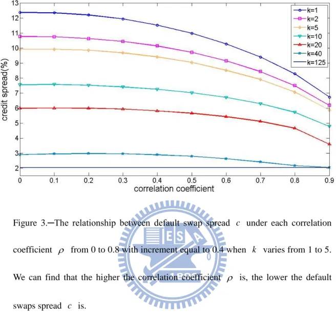
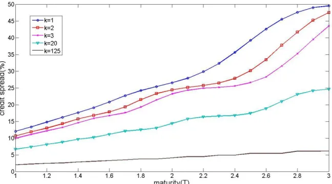
We also show the relationship between correlation coefficient and basket credit spread in Figure 3. Figure 3 tells us that the entities are more related, the basket credit spread also go down more. This result is the consistent as the other literature in previous research. Moreover, it also can found in Figure 4 that if the maturity gets longer, the spread will get larger.

6. Conclusions

Numerical results show that transparency level obviously affects the credit spread of BDS. The relationship between transparency level and basket credit spread is negative, that is, more transparent entities will lead to lower basket credit swap spread. This illustrates us that the investors will ask more premiums to compensate themselves for the low transparency of the entities. The reason is simple: less information means less certainty for investors. When financial statements are not transparent, investors can never be sure about a company's real fundamentals and true

15

risk. For instance, a firm's growth prospects are related to how it invests. It's difficult if not impossible to evaluate a company's investment performance if its investments are funneled through holding companies, making them hidden from view. Lack of transparency may also obscure the company's level of debt. If a company hides its debt, investors can't estimate their exposure to bankruptcy risk. And the entities are more related, the basket credit spread also go down more. Furthermore, the maturity gets longer, the spread will get larger.

16

Reference

Collin D. P., Goldstein R. S., and Martin J. S. (2001) The Determinants of Credit Spread Changes. Journal of Finance, 6, 2177-2207.

Duffie D. and Lando D. (2001) Term Structure of Credit Spreads with Incomplete Accounting Information. Econometrica, 69, 633-664.

Duffie D. (1999) Credit Swap Valuation. Financial Analysts Journal, 55, 73-87. Duffie D. and Singleton, K. (1999) Modeling Term Structures of Defaultable Bonds.

Review of Financial Studies, 12, 687-720.

Edwards A K., Harris L. S. and Piwowar M. S. (2006) Corporate Bond Market Transparency and Transaction Costs. Journal of Finance, 3, 1421 – 1451.

Huang Y. and Neftci S. (2006) Modeling Swap Spreads: The Roles of Credit, Liquidity and Market Volatility. Review of Futures Market, 4, 431-450.

Hull, J. C. (2004) Merton's Model, Credit Risk, and Volatility Skews. Journal of

Credit Risk, 1, 3-28.

In, F., Brown R., and Fang V. (2003) Modeling Volatility and Changes in The Swap Spread. International Review of Financial Analysis, 5, 545-561.

Jarrow R., Lando D., and Turnbull S. (1997) A Markov Model for the Term Structure of Credit Spreads. Review of Financial Studies, 10, 481-523.

17

Wiley and Sons.

Rudiger K., W. Perraudin and Alex T. (2003) The Structure of Credit Risk: Spread Volatility and Ratings Transitions. Risk, 6, 1.

Yu F. (2005) Accounting Transparency and the Term Structure of Credit Spreads.

18

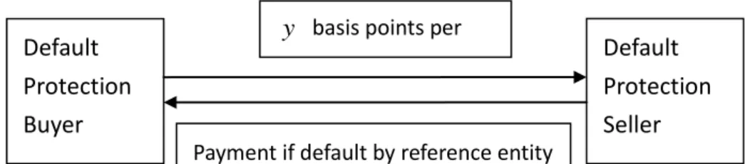
Figure 1. ─Credit default swaps Default Protection Buyer Default Protection Seller

Payment if default by reference entity

y basis points per year

19

Figure 2.─The default swap spread c under each k from 1 to 125 when a varies from 0.05 to 0.25 with increment equal to 0.05 and its correlation coefficient  is 0.8. Obviously, the graph is strictly monotonically decreasing.

20

Figure 3.─The relationship between default swap spread c under each correlation coefficient  _{from 0 to 0.8 with increment equal to 0.4 when k varies from 1 to 5.} We can find that the higher the correlation coefficient  is, the lower the default swaps spread c is.

21

Figure 4.─The relationship between default swap spreads c and maturity when k varies. Each curve is strictly monotonically increasing and it becomes upward when