Multi-table Association Rules Hiding
Shyue-Liang Wang
1and Tzung-Pei Hong
21Department of Information Management
2Department of Computer Science and Information Engineering
National University of Kaohsiung Kaohsiung, Taiwan 81148 {slwang, tphong}@nuk.edu.tw
Yu-Chuan Tsai, Hung-Yu Kao
Department of Computer Science and Information Engineering National Cheng Kung University
Tainan, Taiwan 70101
{p7894131, hykao}@mail.ncku.edu.tw
Abstract
—
Many approaches for preserving association rule privacy, such as association rule mining outsourcing, association rule hiding, and anonymity, have been proposed. In particular, association rule hiding on single transaction table has been well studied. However, hiding multi-relational association rule in data warehouses is not yet investigated. This work presents a novel algorithm to hide predictive association rules on multiple tables. Given a target predictive item, a technique is proposed to hide multi-relational association rules containing the target item without joining the multiple tables. Examples and analyses are given to demonstrate the efficiency of the approach.Keywords- association rule; privacy preserving; hiding; multi-relational; data mining
I. INTRODUCTION
Recent studies in preserving association rule privacy have proposed many techniques [5,8,12,16]. For example, in association rule mining outsourcing, encoding/decoding schemes are developed to transform data and ship it to a third party service provider (server). The data owner sends mining queries to the server and recovers the true patterns from the extracted patterns received from the server. The data mining privacy is protected as the server does not learn any sensitive information from the data. In privacy-preserving data mining, perturbation, and anonymization techniques have been developed to hide the association rules from been discovered form published data.
In particular, for a single data set, given specific rules or patterns to be hidden, many data altering techniques for hiding association rules have been proposed. They can be categorized into three basic approaches. The first approach [3,13] hides one rule at a time. It first selects transactions that contain the items in a give rule. It then tries to modify items, transaction by transaction, until the confidence or support of the rule falls below minimum confidence or minimum support. The modification is done by either removing items from the transaction or inserting new items to the transactions. The second approach deals with groups of restricted patterns or sensitive association rules at a time [11]. It first selects the transactions that contain the intersecting patterns of a group of restricted patterns. Depending on the disclosure threshold given by users, it sanitizes a percentage of the selected transactions in order to hide the restricted patterns. The third approach [14,15] deals with hiding certain constrained classes of association rules. Once the proposed hiding items are given,
the approach integrates the rule selection process into the hiding process. It hides one rule at a time by calculating the number of transactions required to sanitize and modify them accordingly.
However, in real life, a database is typically made up of multiple tables. For example, there are multiple dimension tables and a fact table in a star schema in a data warehouse. Although efficient mining techniques have been proposed to discover frequent itemsets and multi-relational association rules from multiple tables [4,6,7,9,10,17], few works have concentrated on hiding sensitive association rules on multi-relational databases. In this work, we present a novel algorithm for hiding sensitive predictive association rules in data warehouses with star schema. Based on the strategies of no joining of multiple tables and effective reduction of confidence of association rule, the proposed algorithm can effectively hide multi-relational association rules. Examples and analyses are given to demonstrate the efficacy of the approach.
The rest of the paper is organized as follows. Section 2 presents the statement of the problem. Section 3 presents the proposed algorithm for hiding sensitive association rules from multiple tables. Section 4 shows an example of the proposed approach. Section 5 shows the complexity of the proposed algorithm and compares it with joining table approach. Concluding remarks and future works are described in section 6.
II. PROBLEM DESCRIPTION
Association rule mining was first introduced in [1,2]. Let I={i1, i2, …, im} be a set of literals, called items. Given a set of
transactions D, where each transaction T in D is a set of items such that T⊆I, an association rule is an expression X⇒Y where X⊆I, Y⊆I, and X∩Y=∅. The confidence of an association rule is calculated as |X ∪ Y|/|X|, where |X| is the number of transactions containing X and |X∪Y| is the number of transactions containing both X and Y. The support of the rule is the percentage of transactions that contain both X and Y, which is calculated as |X ∪ Y |/N, where N is the number of transactions in D. The problem of mining association rules is to find all rules that are greater than the user-specified minimum support and minimum confidence.
As an example, for a given database with six transactions shown in Figure 1, a minimum support of 33% and a minimum confidence of 70%, nine association rules can be found as follows: B=>A (66%, 100%), C=>A (66%, 100%), B=>C (50%, 75%), C=>B (50%, 75%), AB=>C (50%, 75%), AC=>B (50%, 75%), BC=>A(50%, 100%), C=>AB(50%, 75%), B=>AC(50%,
75%), where the percentages inside the parentheses are supports and confidences respectively.
TID Items T1 {ABC} T2 {ABC} T3 {ABC} T4 {AB} T5 {A} T6 {AC}
Figure 1. A sample dataset
The objective of data mining is to extract hidden or potentially unknown but interesting rules or patterns from databases. However, the objective of privacy preserving data mining is to hide certain sensitive information so that they cannot be discovered through data mining techniques [3,11,13-15]. For association rule hiding, given a transaction database D, a minimum support, a minimum confidence and a set of sensitive association rules X, the objective is to minimally modify the database D such that no association rules in X will be discovered.
Continue from previous example with minimum support 33%, minimum confidence 70%, and a sensitive association rule { C=>B }, if transaction T1 is modified from ABC to AC,
then the rule C=>B (33%, 50%) will be hidden. However, rules B=>C (33%, 66%), AB=>C (33%, 66%), B=>AC (33%, 66%), AC=>B (33%, 50%), C=>AB (33%, 50%),will be lost as side effects.
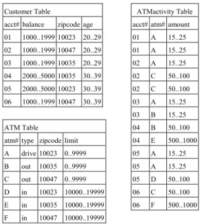
The techniques in association rule mining has been extended to work on numerical data, categorical data, and others in more conventional databases. In a relational database, a set of relational tables may exist. A star schema in a data warehouse is typical made up of multiple dimension tables and a fact table. Consider the following star schema [7] with fact table, ATMactivity(acct#, atm#, amount), and two dimension tables, Customer(acct#, balance, zipcode, age) and ATM(atm#, type, zipcode, limit), as shown in Figure 2. If limited to single table, the association rule mining algorithms on transaction data can be easily extended and discover rules such as: age(20..29) => balance(1000..1999) from table Customer, and type(in) => limit(10000..19999) from table ATM, for each individual table. However, to discover cross table association rules such as limit(0..9999) => balance(1000..1999), limit(0..9999) =>age(20..29), all three tables must be joined. The significant redundancy in such a joined table would seriously degrade the performance of multi-relational association rule mining. To efficiently discover frequent itemsets and association rules across multiple tables, many techniques have been proposed [4,6,7,9,10,17].
In this work, we consider the problem of efficiently hiding predictive association rules on multiple tables in star schema. Given a predictive item, a predictive association rule set is the minimal set of association rules that can make the same prediction as all association rules. For example, given predictive item balance(1000..1999), with min_supp = 0.4 and min_conf=0.6, the predictive association rule set contains two rules: {age(20..29) => balance(1000..1999), limit(0..9999) => balance(1000..1999)}. Even though there may be other rules that contain balance(1000..1999) on the right hand side.
More specifically, given a fact table and a set of dimension tables in a star schema, a minimum support, a minimum confidence, and a predictive item, the objective is to minimally modify the dimension tables such that no predictive association rules will be discovered. For example, given the three tables in Figure 2, minimum support = 0.4, minimum confidence = 0.6, and predictive item balance(1000..1999), if balance(1000..1999) from acct#01 and acct#03 in Customer table are deleted (or suppressed), the two predictive association rules will be hidden.
Customer Table
acct# balance zipcode age 01 1000..1999 10023 20..29 02 1000..1999 10047 20..29 03 1000..1999 10035 20..29 04 2000..5000 10035 30..39 05 2000..5000 10023 30..39 06 1000..1999 10047 30..39 ATMactivity Table acct# atm# amount 01 A 15..25 01 A 15..25 02 A 15..25 02 C 50..100 02 C 50..100 03 A 15..25 03 B 15..25 04 B 50..100 04 E 500..1000 05 A 15..25 05 A 15..25 05 D 50..100 06 C 50..100 06 F 500..1000 ATM Table
atm# type zipcode limit A drive 10023 0..9999 B out 10035 0..9999 C out 10047 0..9999 D in 10023 10000..19999 E in 10035 10000..19999 F in 10047 10000..19999
Figure 2. Fact table and dimension tables in a star schema.
III. PROPOSED ALGORITHM
To hide an association rule efficiently on multiple tables, two issues must be addressed. The first issue is how to calculate supports of itemsets efficiently and the second issue is how to reduce the confidence of an association rule by minimal modification of dimension tables.
To calculate the support of an itemset, one trivial approach is to join all tables together and calculate the supports using any frequent itemset mining algorithm such as Apriori algorithm for transaction data. We assume that quantitative attribute values (e.g. age and monetary amounts) are partitioned and treated as items. It is obvious that joining all tables will increase in size many folds. In large applications, the joining of all related tables cannot be realistically computed because of the many-to-many relationship blow up and large dimensionality. In addition, increase in both size and dimensionality presents a huge overhead to already expensive frequent itemset mining, even if the join can be computed.
Instead of joining-then-mining, we will adopt mining-then-joining approach in this work [7,9].
To reduce the confidence of an association rule X=>Y with minimal modification, the strategy in the support-based and confidence-based distortion schemes is to either decrease its supports, (|X|/N or |X∪Y|/N), to be smaller than pre-specified minimum support or decrease its confidence (|X∪Y|/|X|) to be
smaller than pre-specified minimum confidence.
To decrease the confidence of a rule, two strategies can be considered. The first strategy is to increase the support count of X, i.e., the left hand side of the rule, but not support count of X∪Y. The second strategy is to decrease the support count of the itemset X∪Y. For the second strategy, there are in fact two options. One option is to lower the support count of the itemset X∪Y so that it is smaller than pre-defined minimum support count. The other option is to lower the support count of the itemset X∪Y so that |X ∪Y|/|X| is smaller than pre-defined minimum confidence. In addition, in the record containing both X and Y, if we decrease the support of Y only, it would reduce the confidence faster than reducing the support of X. In fact, we can pre-calculate the number of records required to hide the rule. If there is not enough record to lower the confidence of the rule, then the rule cannot be hidden. To decrease support count of an item, we will remove one item at a time in the selected record by deleting it or suppressing it (replaced by *). In this work, we will adopt the second strategy for the proposed algorithm.
In order to hide predictive association rules, we will consider hiding association rules with 2 items, x=>z, where z is a predictive item and x is a single large one item. In theory, predictive association rules may have more specific rules that contain more items, e.g., xY => z, where Y is a large itemset. However, for such rule to exist, its confidence must be greater than the confidence of x=>z, i.e., conf(xY=>z) > conf(x=>z) or |xYz| > conf(x=>z) * |xY|. For higher confidence rules, such as conf(x=>z) = 1, there will be no more specific rules. In addition, once the more general rule is hidden, the more specific rule might be hidden as well.
Algorithm HPAR
Input: (1) a fact table FT, and a set of dimension tables DT1,
DT2…,
(2) minimum support (min_supp), (3) minimum confidence (min_conf), (4) a set of hidden items Y,
Output: fact table and a transformed set of dimension tables
where the predictive association rules containing Y on the RHS are hidden.
1. Find all frequent 1-itemsets; //scan FT, build vector vt for
each FK and TID lists for each item; 2. For each frequent target item y in Y,
2.1 Find all in-table frequent 2-itemsets containing target item y; //use TID list
2.2 Find all cross-table frequent 2-itemsets containing target item y; // scan FT and build vector ct
2.3 Calculate the confidences of all predictive association rules, x=>y; // Conf(x=>y) >= min_conf
2.4 Sort the PARs in descending order of confidence; 2.5 Repeat
2.5.1 Get the first PAR;
2.5.2 Calculate the number of records, iterNum, needs to be modified; // for confidence to be smaller than min_conf or support to be smaller than min_supp; 2.5.3 Find the TIDs containing target item with sum of vt
counts >= iterNum;
2.5.4 Delete the target item in the TIDs;
2.5.5 Update the confidences of PARs; 2.5.6 Sort the PARs in descending order; 2.6 Until (no more PAR);
The HPAR algorithm first tries to find all frequent 1-itemsets from one scan of fact table by building a vector vt to record the
support counts for the primary key values of dimension tables. It also records the TID list for each 1-itemset. It then tries to find all frequent 2-itemsets by scanning the fact table to calculate the support counts for cross-table itemsets. The in-table 2-itemsets can be calculated by performing intersection on TID lists in the same dimension table. To hide a predictive association rule, the algorithm calculates the number of records required to be modified and perform deletion (or suppression). It repeats the same process after modification and update until no more predictive association exists.
IV. EXAMPLE
This section shows an example to demonstrate the proposed algorithm in hiding predictive association rules from multiple tables of star schema.
Given dimension tables Customer, ATM, fact table ATMactivity with min_support = 0.4, min_conf=0.6, and hidden item = {balance(1000..1999)}, the execution of the proposed algorithm is shown as follows.
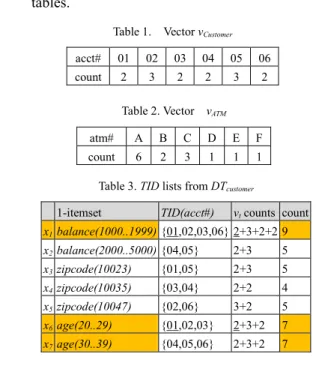
Step 1: Scan fact table to build vt for each FK acct# and atm#,
and build TID lists for each 1-itemset in dimension tables.
Table 1. Vector vCustomer
acct# 01 02 03 04 05 06 count 2 3 2 2 3 2
Table 3. TID lists from DTcustomer
1-itemset TID(acct#) vt counts count x1balance(1000..1999) {01,02,03,06} 2+3+2+2 9 x2balance(2000..5000) {04,05} 2+3 5 x3zipcode(10023) {01,05} 2+3 5 x4zipcode(10035) {03,04} 2+2 4 x5zipcode(10047) {02,06} 3+2 5 x6age(20..29) {01,02,03} 2+3+2 7 x7age(30..39) {04,05,06} 2+3+2 7
Table 2. Vector vATM
atm# A B C D E F count 6 2 3 1 1 1
Table 4. TID lists from DTATM
TID Acct# 01,02,03,06
ATM# 2-itemset balance(1000..1999) A type(drive) 3 A,D zipcode(10023) 3 A.B,C limit(0..9999) 8
The six frequent 1-itemsets are { balance(1000..1999), age(20..29), age(30..39), type(drive), zipcode(10023), limit(0..9999)}.
Step 2: For hidden item balance(1000..1999), which is frequent, the in-table candidate 2-itemsets containing balance(1000..1999) are:
Table 5. In-table candidate 2-itemsets
2-itemsets TID vt count
balance(1000..1999),age(20..29) 01,02,03 2+3+2 7 balance(1000..1999),age(30..39) 06 2 2
The TIDs of a 2-itemset can be calculated directly by the intersection of two TID lists of 1-itemsets.
The cross-table frequent 2-itemsets containing target item balance(1000..1999) can be determined by scanning FT and calculate the support counts of the following 2-itemset in table ct. It is seen that there is one in-table frequent itemset { balance(1000..1999), age(20..29)} and one cross-table frequent itemset { balance(1000..1999), limit(0..9999)}. The sorted predictive association rules are age(20..29) => balance(1000..1999)[50%, 100%], limit(0..9999) => balance(1000..1999)[57%, 73%].
Table 6. Cross-table frequent 2-itemsets
TID Acct# 01,02,03,06
ATM# 2-itemset balance(1000..1999) A type(drive) 3 A,D zipcode(10023) 3 A.B,C limit(0..9999) 8
To hide the rule age(20..29) => balance(1000..1999), we need to delete at least 3 records with balance(1000..1999) such that its confidence is less than min_confidence 0.6. This is because ⎡|FT|*(supp(xy) - min_conf * supp(x))⎤ = 14*(7/14 – 0.6*7/14) = 3. From the TID list of 1-itemset balance(1000..1999), we find acct#01, acct#3 both appear twice in fact table. This is the minimal number of target item we can delete in order to hide the specified rule. Therefore we delete balance(1000..1999) from acct#01 and acct#3 in the dimension table DT1. The confidence of rule becomes 3/7≈ 0.43 and is
therefore hidden. In addition, the updated confidence of the rule limit(0..9999) => balance(1000..1999) becomes 4/11≈ 0.36 and is also hidden. The algorithm stops as both predictive association rules are hidden after deleting balance(1000..1999) form acct#1 and acct#3 from dimension table Customer.
V. ANALYSIS
In this section, we provide complexity analyses on the proposed algorithm and compare it with joining-then-mining approach.
Instead of calculating and hiding predictive association rules on the joined table formed by fact table and all dimension tables, the proposed algorithm find the association rules in two phases similar to [7]. It first calculates all 1-itemsets by one scan of fact table. It then calculates all 2-itemsets, both in-table and cross-table, by another scan of fact table, without performing join operation and materialize the join. For each predictive association rule, it calculates the number of records that need to be modified. The process is repeated after modification and update until all rules are hidden. We first provide the calculation of number of modification required and then estimate the operation on itemsets required to hide the predictive association rules.
Lemma 1: For a predictive association rule x=>y, y
∈
Y,algorithm HPAR performs min (⎡|FT|*(supp(xy) - min_conf * supp(x))⎤ , ⎡|FT|*(supp(xy) - min_supp)⎤) modifications to hide the rule.
Proof. Line 2.5.2 calculates the number of records that
needs to be modified so that the confidence of a given rule is either smaller than min_conf or support to be smaller than min_supp. Let the confidence of a predictive association rule be |xy|/|x| and greater than min_conf. The support count of |xy| is decreased by one when one transaction containing xy is modified to support x only. Assuming it takes k1 executions to
reduce the confidence to be less than min_conf, i.e., (|xy| – k1)/|x| < min_conf. This inequality can be rewritten as k1 =
⎡|xy| - min_conf *|x|⎤ = ⎡|FT|*(supp(xy) - min_conf * supp(x))⎤ . Assuming it takes k2 executions to reduce the
support to be less than min_supp, i.e., (|xy| – k2)/|FT| <
min_supp. This inequality can be rewritten as k2 = ⎡|xy| -
min_supp *|FT|⎤ = ⎡|FT|*(supp(xy) - min_supp)⎤ . Therefore, it would take min(k1, k2) modifications to hide the rule, since
either the confidence is less than the min_conf or the support is less than min_supp.□
Lemma 2: The time complexity of HPAR algorithm is
O(|FT| + |Y|*(|FT|+(l22*logl2) /2)), where |FT| is the number of
records in fact table, |Y| is the number of items in Y, and l2 is the
maximum number of frequent 2-itemsets.
Proof. The time complexity estimated here is based on the
number of operations required on itemsets. To find all frequent 1-itemsets in line one, it takes O(|FT|) operations. On line two, there are at most |Y| number of frequent target items. For each of these items, the following operations are executed. To find frequent 2-itemsets, it is line 2.2 that calculating cross-table itemsets will require most operations. It takes O(|FT|) operations to scan the fact table again. Assuming the maximum number of frequent 2-itemset is l2, step 2.4 and step
2.5.6 perform sorting of these frequent 2-itemsets repeatedly. It would require O((l22*logl2) /2) operations. In total, the
estimated operation is O(|FT| + |Y|*(|FT|+(l22*logl2) /2)) .□
For joining-then-mining approach, a straight forward calculation of predictive association rule is to join the fact table with all dimension tables and then perform Apriori algorithm. Let JT = FT DT1 ... DTn be the joined table. If we
apply same strategy to reduce the confidence of an association rule, then time complexity can be estimated similarly.
Lemma 3: The time complexity of joining-then-hiding
approach is O(|JT| + |Y|*(|JT|+(l22*logl2) /2)), where |JT| is the
number of records in fact table, |Y| is the number of items in Y, and l2 is the maximum number of frequent 2-itemsets.
Proof. The proof is similar to lemma 2. □
It can be observed that the joined table JT is much bigger than the fact table FT, as JT contains attributes from all dimension tables. The operations on joined table will be much more than operations on fact table along. In addition, the cost of joining and memory space to save the joined table must be considered.
VI. CONCLUSION
In this work, we have studied the problem of hiding sets of predictive association rules on multiple tables of star schema. We propose a novel technique addressing two issues – efficient calculation of itemsets and reduction of rule confidence. Examples illustrating the proposed approach are shown. Analyses are given and compared to joined table approach. Currently we have implemented the proposed technique on single table and experimenting on multiple tables. We will continue to examine and improve the various side effects of the proposed approach. We will also consider utilizing better data structures to reduce database scanning for better efficiency.
ACKNOWLEDGMENTS.
This work was supported in part by the National Science Council, Taiwan, under grant NSC-98-2221-E-390-030.
REFERENCES
[1] R. Agrawal, T. Imielinski and A. Swami, “Mining Association Rules between Sets of Items in Large Databases”, Proceedings of ACM SIGMOD International Conference on Management of Data, 207–216,
1993.
[2] R. Agrawal and R. Srikant. “Fast Algorithms for Mining Association Rules in Large Databases”, Proceedings of the 20th International Conference on Very Large Data Bases, VLDB, 487-499, 1994.
[3] E. Dasseni, V. Verykios, A. Elmagarmid and E. Bertino, “Hiding Association Rules by Using Confidence and Support” in Proceedings of 4th Information Hiding Workshop, 369-383, Pittsburgh, PA, 2001. [4] L. Dehaspe and L. De Raedt. “Mining Association Rules in Multiple
Relations”, Proceedings of the 7th International Workshop on Inductive Logic Programming, 125–132. 1997.
[5] F. Giannotti, L.V.S. Lakshmanan, A. Monreale, D. Pedreschi, and H. Wang, “Privacy-preserving Mining of Association Rules from Outsourcing Transaction Databases”, position paper in Workshop on Security and Privacy in Cloud Computing, in conjunction with the International Conference on Computers, Privacy and Data Protection, January, 2010. [6] J.F. Guo, W.F. Bian, and J. Li, “Multi-relational Association Mining with
Guidance of User”, Proceedings of the Fourth International Conference on Fuzzy Systems and Knowledge Discovery, 704-709, 2007.
[7] V. C. Jensen, N. Soparkar, “Frequent Itemset Counting Across Multiple Tables”, Proceedings of the 4th Pacific-Asia Conference of Knowledge Discovery and Data Mining, Current Issues and New Applications, 49−61, 2000.
[8] I. Molloy, N. Li, and T. Li, “On the (In)Security and (Im)Practicality of Outsourcing Precise Association Rule Mining”, Proceedings of International Conference on Data Mining, 2009.
[9] K.K. Ng, W.C. Fu, K. Wang, “Mining Association Rules from Stars”,
Proceedings of the 2002 IEEE International Conference on Data Mining, 322−329, 2002.
[10] S. Nijssen and J. Kok, “Faster Association Rules for Multiple Relations”, Proceedings of the 17th International Joint Conference on Artificial Intelligence, 891−896, 2001.
[11] S. Oliveira, O. Zaiane, “Algorithms for Balancing Privacy and Knowledge Discovery in Association Rule Mining”, Proceedings of 7th International Database Engineering and Applications Symposium, Hong Kong, July 2003.
[12] L. Qiu, Y. Li, X. Wu, “Protecting Business Intelligence and Customer Privacy while Outsourcing Data Mining Tasks”, Knowledge and Information Systems, Vol. 17, 1, 99-120, 2008.
[13] V. Verykios, A. Elmagarmid, E. Bertino, Y. Saygin, and E. Dasseni, “Association Rules Hiding”, IEEE Transactions on Knowledge and Data Engineering, Vol. 16, No. 4, 434-447, April 2004.
[14] S.L. Wang, D. Patel, A. Jafari, and T.P. Hong, “Hiding Collaborative Recommendation Association Rule”, Applied Intelligence, Volume 27, No. 1, 67-77, August 2007.
[15] S.L. Wang, T.Z. Lai, T.P. Hong, and Y.L. Wu, “Hiding Collaborative Recommendation Association Rules on Horizontally Partitioned Data”, Intelligent Data Analysis, Vol. 14, No. 1, January 2010, 47 – 67.
[16] W.K. Wong, D.W. Cheung, E. Hung, B. Kao, and N. Mamoulis, “Security in Outsourcing of Association Rule Mining”, Proceedings of International Conference on Very Large Data Bases, 2007.
[17] L.J. Xu, K.L. Xie, “A Novel Algorithm for Frequent Itemset Mining in Data Warehouses”, Journal of Zhejang University Science A, 7(2), 216-224, 2006.