以潛在類別方法評估精神分裂症活性與負性症狀之潛在結構與轉變

全文

(1)國立交通大學統計學研究所碩士論文以潛在類別方法評估精神分裂症活性與負性症狀之潛在結構與轉變 Evaluation of Latent and Transition Structures of Positive and Negative Syndrome Scale (PANSS) in Schizophrenia using Regression Extension of Latent Class Analysis and Latent Transition Analysis. 研究生：蔡秀慧指導教授：黃冠華博士. 中華民國九十五年六月.

(2) 以潛在類別方法評估精神分裂症活性與負性症狀之潛在結構與轉變 Evaluation of Latent and Transition Structures of Positive and Negative Syndrome Scale (PANSS) in Schizophrenia using Regression Extension of Latent Class Analysis and Latent Transition Analysis 研究生：蔡秀慧指導教授：黃冠華. Student：Hsiu-Hui Tsai Advisor：Dr. Guan-Hua Huang. 國立交通大學統計學研究所碩士論文 A Thesis Submitted to Institute of Statistics College of Science National Chiao Tung University in Partial Fulfillment of the Requirements for the Degree of Master in Statistics June 2006. Hsinchu, Taiwan, Republic of China 中華民國九十五年六月.

(3) 以潛在類別方法評估精神分裂症活性與負性症狀之潛在結構與轉變研究生：蔡秀慧. 指導教授：黃冠華博士. 國立交通大學統計學研究所. 摘要本研究有兩個主要目的：一是探討精神分裂症之活性與負性症狀評量表(PANSS)的結構，一是深入研究在不同階段下結構的轉變。我們以潛在類別迴歸方法找出 219 位急性期精神分裂症患者可分為五種類別：混合、負性、解組性思考、妄想及活性/少數混合，並找出 225 位慢性期精神分裂症患者可區分為四種類別：少數混合、負性、妄想及無症狀，根據研究發現慢性期的症狀結構是附屬在急性症狀期的症狀結構之下。另外，以潛在變遷分析探討 115 位精神分裂症患者在急性與慢性期的結構轉變，我們發現兩階段的症狀結構皆有負性類別，且大多數在急性期屬於負性類別的病患，在慢性期仍會保留在負性類別中，顯示負性症狀不易治癒的可能性。. 關鍵字：結構、症狀、精神分裂症、活性與負性症狀評量表、急性期、慢性期、潛在類別迴歸、潛在變遷分析. i.

(4) Evaluation of Latent and Transition Structures of Positive and Negative Syndrome Scale (PANSS) in Schizophrenia using Regression Extension of Latent Class Analysis and Latent Transition Analysis.. Student: Hsiu-Hui Tsai. Advisor: Dr. Guan-Hua Huang. Institute of statistics National Chiao Tung Unerversity. Abstract The main aim of the study is to examine the structure of the PANSS items by using the regression extension of latent class analysis (RLCA) and focuses mainly on the changes in latent class of the PANSS over time. The RLCA identified five-class labeled as mixed, negative, disorganized thought, delusion and positive/a little mixed on 219 acute patients, and identified four-class labeled as a little mixed, negative, delusion and no-symptoms on 225 chronic patients. Based on the research, it was indicated that the symptom structure on the chronic schizophrenia was nested within the symptom structure on the acute schizophrenia. In addition, the latent transition analysis (LTA) was carried out to examine the changes of latent class on 115 patients who had assessed PANSS in both two phases. We found that the component of the negative class was stability over time and most patients who belonged to the negative class in the acute phase would still retain in the negative class in the chronic phase. It shows the possibility that the negative symptoms are difficult to cure. Key words: Structure, Symptoms, Schizophrenia, PANSS, Regression extension of latent class analysis (RLCA), Latent transition analysis (LTA), Acute, Chronic.. ii.

(5) 誌. 謝. 在統研所兩年，有快樂也有痛苦的事，許許多多的回憶點滴在心頭，快樂的事就是有一群可愛的同學，痛苦的事莫過於生論文與念看不懂的 paper；在此非常感謝黃冠華老師在這兩年內不辭辛勞的指導，老師雖然很忙，但是仍盡力幫我找答案，適時給我鼓勵與支持，讓我不至於像我研究的主題一樣得精神分裂症，讓我能順利的撐過這兩年，一切都是老師您的幫助，所以，在此要跟您說一聲，「老師，謝謝您，您辛苦了。」也要謝謝所上的老師們在這兩年內的指導，讓我對統計有更深入的研究與瞭解；更謝謝台大醫院精神科提供資料讓我們研究分析，沒有可貴的資料，就沒有這份研究；還有要謝謝口試委員在口試時給我意見與建議，讓我的論文能更完整、更充實。另外，也要謝謝陪我走過這兩年的好姐妹們，鷰筑、大宛、孟樺、小宛、沛君、婉文與小馬，讓我的研究生涯不至於被煩惱包圍，讓我生活增添許多樂趣，真的很高興與認識妳們。再來，要感謝與我同個指導教授的志強，謝謝你在我苦惱論文生不出、程式跑不完時，給我的鼓勵與支持，也謝謝你時常幫我翻譯英文，幫我計算一些複雜的數學式子。我還要感謝我的五專同學-佩馨，辛苦的幫我校稿，修改我的英文論文，還有陪我走過許多日子的小玉、章魚、珮怡、佳永、偉孝及台北的朋友們：鍾阿姨、聿芯、曉蕾、伉媖、佳玲、怡靜，感謝妳們總是陪在我身旁，陪我渡過無數個開心與挫折的日子，真的好感謝老天讓我認識了你們，因為你們讓我的生活更快樂也更充實。在此，僅以此篇論文獻給我的好友們，謝謝你們。. 蔡秀慧. 謹誌于. 國立交通大學統計研究所中華民國九十五年六月. iii.

(6) Contents Abstract(in Chinese). i. Abstract(in English). ii. Acknowledgements(in Chinese). iii. Contents. iv. List of Tables. vi. List of Figures. ix. 1 Introduction. 1. 2 Model Literature Review. 5. 2.1. Regression Extension of Latent Class Analysis (RLCA) . . . . . . . . . . .. 5. 2.2. Latent Variable Mixture Modeling for Categorical Data . . . . . . . . . . .. 6. 2.3. Latent Transition Analysis . . . . . . . . . . . . . . . . . . . . . . . . . . .. 8. 2.4. Model estimation and assessment . . . . . . . . . . . . . . . . . . . . . . .. 9. 3 Latent Structure of PANSS. 12. 3.1. Background . . . . . . . . . . . . . . . . . . . . . . . . . . . . . . . . . . . 12. 3.2. Method . . . . . . . . . . . . . . . . . . . . . . . . . . . . . . . . . . . . . 14. 3.3. 3.2.1. Subjects . . . . . . . . . . . . . . . . . . . . . . . . . . . . . . . . . 14. 3.2.2. Instruments . . . . . . . . . . . . . . . . . . . . . . . . . . . . . . . 16. 3.2.3. Study Variables . . . . . . . . . . . . . . . . . . . . . . . . . . . . . 17. 3.2.4. Regression Extension of Latent Class Analysis (RLCA) . . . . . . . 20. 3.2.5. Analytic Strategy . . . . . . . . . . . . . . . . . . . . . . . . . . . . 21. Results . . . . . . . . . . . . . . . . . . . . . . . . . . . . . . . . . . . . . . 23 iv.

(7) 3.4. 3.3.1. Selecting the Number of Latent Classes . . . . . . . . . . . . . . . . 23. 3.3.2. Results of the Latent Class Model . . . . . . . . . . . . . . . . . . . 24. 3.3.3. Comparison of Component of Structure for the PANSS . . . . . . . 34. Discussion . . . . . . . . . . . . . . . . . . . . . . . . . . . . . . . . . . . . 37. 4 Transition of Structure on PANSS. 41. 4.1. Background . . . . . . . . . . . . . . . . . . . . . . . . . . . . . . . . . . . 41. 4.2. Method . . . . . . . . . . . . . . . . . . . . . . . . . . . . . . . . . . . . . 43 4.2.1. Subjects . . . . . . . . . . . . . . . . . . . . . . . . . . . . . . . . . 43. 4.2.2. Instruments . . . . . . . . . . . . . . . . . . . . . . . . . . . . . . . 45. 4.2.3. Study Variables . . . . . . . . . . . . . . . . . . . . . . . . . . . . . 46. 4.2.4. Latent Transition Analysis . . . . . . . . . . . . . . . . . . . . . . . 48. 4.2.5. Analytic Strategy . . . . . . . . . . . . . . . . . . . . . . . . . . . . 49. 4.3. Results . . . . . . . . . . . . . . . . . . . . . . . . . . . . . . . . . . . . . . 51. 4.4. Discussion . . . . . . . . . . . . . . . . . . . . . . . . . . . . . . . . . . . . 59. 5 Conclusion. 61. References. 62. v.

(8) List of Tables Table 1: Characteristics of two groups of patients in the MPGRP project. ............................72 Table 2: Characteristics of the participants in the acute or chronic phase..............................73 Table 3: Characteristics of the PANSS for the acute or chronic phase...................................74 Table 4: AIC, BIC criteria and the number of fixed parameters in the acute and chronic phases under the latent class model without incorporated covariates. ..............................75 Table 5: Final class proportions for the latent classes based on the estimated model. ...........76 Table 6: The summary results of the acute phase with the latent five-class model without covariates using our program. ...........................................................................................77 Table 7: The summary results of the acute phase with the latent five-class model without covariates using Mplus. .....................................................................................................78 Table 8: The summary results of the acute phase with the latent five-class model with demographic variables using our program. .......................................................................79 Table 9: The summary results of the acute phase with the latent five-class model with demographic variables using Mplus. .................................................................................80 Table 10: The summary results of the acute phase with the latent five-class model with environmental factors adjusted significant demographic variables using our program. ...81 Table 11: The summary results of the acute phase with the latent five-class model with environmental factors adjusted significant demographic variables using Mplus..............82 Table 12: The summary results of the acute phase with the latent five-class model with the undegraded d’ of the CPT performance adjusted significant demographic variables using our program. ......................................................................................................................83 Table 13: The summary results of the acute phase with the latent five-class model with the undegraded d’ of the CPT performance adjusted significant demographic variables using Mplus.................................................................................................................................84 Table 14: The summary results of the acute phase with the latent five-class model with Table 4: the degraded d’ of the CPT performance adjusted significant demographic variables using our program..............................................................................................................85 Table 15: The summary results of the acute phase with the latent five-class model with the degraded d’ of the CPT performance adjusted significant demographic variables using Mplus.................................................................................................................................86 Table 16: The summary results of the chronic phase with the latent four-class model without covariates using our program. ...........................................................................................87 Table 17: The summary results of the chronic phase with the latent four-class model without covariates using Mplus. .....................................................................................................88 Table 18: The summary results of the chronic phase with the latent four-class model with demographic variables using our program. .......................................................................89 Table 19: The summary results of the chronic phase with the latent four-class model with. vi.

(9) demographic variables using Mplus. .................................................................................90 Table 20: The summary results of the chronic phase with the latent four-class model with environmental factors adjusted significant demographic variables using our program. ...91 Table 21: The summary results of the chronic phase with the latent four-class model with environmental factors adjusted significant demographic variables using Mplus..............92 Table 22: The summary results of the chronic phase with the latent four-class model with the undegraded d’ of the CPT performance adjusted significant demographic variables using our program. ......................................................................................................................93 Table 23: The summary results of the chronic phase with the latent four-class model with the degraded d’ of the CPT performance adjusted significant demographic variables using our program..............................................................................................................................94 Table 24: The summary results of the chronic phase with the latent four-class model with the number of categories completed of the WCST adjusted significant demographic variables using our program..............................................................................................................95 Table 25: The summary results of the chronic phase with the latent four-class model with the perseverative errors of the WCST adjusted significant demographic variables using our program..............................................................................................................................96 Table 26: The summary results of the chronic phase with the latent four-class model with the perseverative errors of the WCST adjusted significant demographic variables using Mplus.................................................................................................................................97 Table 27: The summary results of the chronic phase with the latent four-class model with the full scale IQ of the WAIS-R adjusted significant demographic variables using our program..............................................................................................................................98 Table 28: The summary results of the chronic phase with the latent four-class model with the full scale IQ of the WAIS-R adjusted significant demographic variables using Mplus. ...99 Table 29: The summary results of the chronic phase with the latent four-class model with the sum of WMS-R Logical Memory I and Logical Memory II adjusted significant demographic variables using Mplus. ...............................................................................100 Table 30: The summary results of the chronic phase with the latent four-class model with the TMT-A adjusted significant demographic variables using our program. ........................101 Table 31: The summary results of the chronic phase with the latent four-class model with the TMT-A adjusted significant demographic variables using Mplus...................................102 Table 32: The summary results of the chronic phase with the latent four-class model with the TMT-B adjusted significant demographic variables using our program. ........................103 Table 33: The summary results of the chronic phase with the latent four-class model with the TMT-B adjusted significant demographic variables using Mplus...................................104 Table 34: Comparison of structure for the PANSS items for the present study with other studies. .............................................................................................................................105 Table 35: Characteristics of the participants who assessed the PANSS in the both two phases.. vii.

(10) .........................................................................................................................................109 Table 36: Characteristics of the PANSS for the participants who assessed the PANSS in the both two phases. .............................................................................................................. 110 Table 37: The summary resulting from LTA without covariates. ......................................... 111 Table 38: The summary resulting from LTA with demographic variables. .......................... 113 Table 39: The summary resulting from LTA with significant demographic variables and environmental factors. ..................................................................................................... 115 Table 40: The summary resulting from LTA with significant demographic variables and the undegraded d’ of the CPT performance........................................................................... 117 Table 41: The summary resulting from LTA with significant demographic variables and the degraded d’ of the CPT performance............................................................................... 119. viii.

(11) List of Figures Figure 1: AIC and BIC criteria for selecting the number of classes in the acute and chronic phases. .............................................................................................................................121. ix.

(12) 1. Introduction. Schizophrenia is a psychotic disorder characterized by several sets of symptoms, according to the criteria of the Diagnostic and Statistical Manual of Mental of Disorders (4th ed., DSM-IV; American Psychiatric Association, 1994). Many studies have examined the structure of symptoms in schizophrenia. Since Crow proposed the two-factor concept of schizophrenia in 1980 (Crow et al., 1980), researchers began to produce evidence for a syndromic dichotomy (negative-positive) (Bilder et al.,1985; Cornblatte et al., 1985; Andreasen and Grove, 1986; Kay and Sevy, 1990; Mortimer et al., 1990). The positive symptoms, such as hallucinations and delusions, represent a behavioral excess generally considered psychotic. In contrast, negative symptoms, such as blunted affect and passive social withdrawal, represent a deficiency in normal behavior. Although many of these investigations developed the symptom structures from Crow’s original two-dimension distinction and others also found that more than two components are needed to describe the symptoms in Schizophrenia (Liddle, 1987; Arndt et al., 1991; Andreason et al.,1995; Lindenmayer et al., 1995; Lenzenweger and Dworkin, 1996; Johnstone and Frith, 1996), such as Liddle (1987) proposed the disorganization symptoms. A recent study suggested that a four-factor model fit as well as two- and three- factor models (Dollfus and Everitt, 1998). However, the study was limited by the heterogeneity of patients in acute and stabilized phases and its lack of validation by follow-up data. Some instruments were developed for measuring and quantifying different symptom dimensions, such as the Assessment of Negative Symptoms (SANS; Andreasen, 1983), the Scale for the Assessment of Positive Symptoms (SAPS; Andreasen, 1984) and the Positive and Negative Syndrome Scale (PANSS; Kay et al., 1987). The SANS and SAPS were designed to measure Positive and Negative syndromes. These instruments may be limited in their potential to identify schizophrenia subtypes because of the prior selection of symptoms. The PANSS is a more extensive assessment of the symptom phenomenology. 1.

(13) of schizophrenia. It was developed by Kay et al. used the Brief Psychiatric Rating Scale (BPRS; Overall and Gorham, 1962) and the Psychopathology Rating Schedule (PRS; Singh and Kay, 1979). The PANSS provides well-defined operational criteria for symptom assessment yielding good to excellent inter-rater reliability. It demonstrates better interrater reliability and greater predictive power than the BPRS (Bell et al., 1992) and has been an effective research tool in a wide range of studies (Kay, 1990). A number of studies performed exploratory factor analyses (EFA; Lin et al., 1996, 1998), confirmatory factor analysis (CFA; Dollfus and Everitt, 1998), or cluster analysis (Dollfus et al., 1996) for unraveling the structure of the PANSS items. White et al. (1997) fitted 20 previously proposed models to data from a sample of 1,233 schizophrenics for attempt to reconcile the different research finds. They concluded that none of these models fitted the data adequately, then they derived a new ”pentagonal” model retaining only 25 items of the PANSS, which were labeled: Positive, Negative, Dysphoric mood, Activation, and Autistic preoccupation, and it’s presently proposed in the manual for the PANSS (Kay et al., 2000). However, the study by White et al. did not finish the argument surrounding the factor structure of the PANSS. Critics argued that the structure of the PANSS items may not be best represented by five components (Emsley et al., 2003), and the proposed pentagonal model had inadequate goodness of fit in other samples (Lykouras et al., 2000; Fitzgerald et al., 2003). Differences in patient characteristics and symptom ensembles assessed might partly account for the discrepancies. In addition, the inclusion of patients at different stages of the disease may constitute another source of bias. This study was conducted in schizophrenic patients at various progressive stages of the disease. We conducted a study in two distinct populations of schizophrenic patients, one in the acute, and the other in the chronic stage. On the other hand, most studies that examined the symptom components in schizophrenia suffered from the limitation that symptoms were measured only cross-sectionally. 2.

(14) Therefore, how the composition of the symptom components changes over time remains unknown. Kulhara and Chandiramani (1990) found 98 schizophrenic inpatients could divided into three symptom factors (negative symptoms, positive symptoms, thought disorder). However, 18-30 months later, 79 of these patients were reassessed and the composition of these symptom factors had changed, which was that a mixed symptom factor replayed the positive symptom factor. Goldman et al. (1991) reported that at both time, which were prior to intervention (medication-free baseline) and after 4 weeks of neuroleptic treatment, three symptom factor were evident (negative symptoms, positive symptoms, and unstable behavioral agitation) and that the pre- and post-treatment factor loading patterns were similar in 40 schizophrenic inpatients. Addington and Addington (1991) found two symptom factors having eigenvalues greater than unity (negative symptoms and thought disorder) in 41 schizophrenic inpatients at beginning of the study. However, after 6 months, the reality distortion factor appeared in place of the thought disorder. Van der Does et al. (1995) rated 65 schizophrenic patients at the acute phase, 3 months later, and 1 year after the second assessment. They found that there was a different factor structure at each assessment, but a four-dimensional structure (disorganization, negative symptoms, positive symptoms, and depression) was stable over time. According to a study of Nakaya et al. (1999) with 86 newly admitted schizophrenic patients, four symptom factors were observed in the acute phase (negative symptoms, excited, delusion/hallucinatory, and thought disorder). However, in the post-acute phase, three symptom factors were evident (negative symptoms, mixed symptoms, and though disorder). They suggested that the negative symptom component is stable while the difference in the phase of illness has some effects on the symptom structure of schizophrenia. Therefore, each previous study produces different findings about the composition of symptom components over time and the sampling and assessment methods differed among the previous studies, making any comparison difficult. Although a part of previous studies explored the symptomatology of schizophrenia in different phase, but how the patients will change between the acute 3.

(15) phase and the chronic phase, that remains unknown. In present, there are two main researches included in the study. One is to examine the structure of the PANSS items by using the regression extension of latent class analysis (RLCA, Huang and Bandeen-Roche, 2004), which is useful for classifying subjects based on their responses to a set of categorical items. Another focuses on the changes in latent class of the PANSS over time. First, the number of classes for two distinct phases of the disease will be selected based on AIC and BIC criteria. Second, according to the number of classes obtained in first step, the regression extension of latent class analysis (RLCA, Huang and Bandeen-Roche, 2004) will be performed to classify schizophrenic patients at two distinct phases (acute and chronic) of the disease. In addition, we will perform RLCA with demographic variables, environmental factors or neuropsychological variables to explore the relation between the latent class and demographic variables, environmental factors or neuropsychological variables. On the other hand, the structure of the PANSS in this study is compared with the structure of the PANSS in the previous studies. Third, the changes in the structure of the PANSS items in both the acute phase and the chronic phase will be examined by applying latent transition analysis (LTA). Besides, we will perform LTA with demographic variables, environmental factors or neuropsychological variables to explore the changes of the structure of the PANSS after adjusting demographic variables, environmental factors or neuropsychological variables.. 4.

(16) 2. Model Literature Review. 2.1. Regression Extension of Latent Class Analysis (RLCA). Let (Yi1 , · · · , YiM )T represent the M × 1 response vector and Si denote the unobservable latent categorical variables, for the ith individual in a study sample of N persons. Yim can take values {1, · · · , Km }, where Km ≥ 2, m = 1, · · · , M , and Si can take values {1, · · · , J}. The LCA model is based on the concept of conditional independence in the sense that the measured indicators are assumed to be independent of one another within any category of the latent variable. Therefore, the distribution for (Yi1 , · · · , YiM ) can be expressed as Pr(Yi1 = y1 , · · · , YiM = ym ) =. J X. M K m Y Y. {P r(Si = j). [P r(Yim = k|Si = j)]ymk },. (1). m=1 k=1. j=1. where, ymk = 1 if ym = k; 0 otherwise. The LCA model assumes that Pr(Yim = k|Si = j) = pmkj , P r(Si = j) = ηj ,. (2). Thus, ηj are the “latent class probabilities” of each underlying variable category, and pmkj are the “conditional probabilities” of the measured responses given the underlying variable category. To incorporate covariate effects into LCA, let xi be the associated covariate vector for the ith person, where xi = (xi1 , · · · , xiP )T are predictors associated with latent class Si . The covariates may include any combination of continuous and discrete measures. The Regression Extension of Latent Class Analysis (RLCA) is then stated as Pr(Yi1 = y1 , · · · , YiM = ym |xi ) =. J X. {ηj (xi ). j=1. M K m Y Y. [pmkj ]ymk },. (3). m=1 k=1. with ηj (xi ) defined as in the generalized linear framework (McCullagh and Nelder, 1989). Often, (3) is implemented assuming generalized logit (Agresti, 1984) link functions: log[. ηj (xi ) 0 ] = αj + β1j xi1 + · · · + βP j xiP = αj + β j xi , ηJ (xi ). (4). pmkj 0 ] = γmkj 0 , pmKm j 0. (5). and log[. 5.

(17) 0. i = 1, · · · , N ; m = 1, · · · , M ; k = 1, · · · , Km − 1; j = 1, · · · , J − 1; j = 1, · · · , J. Through (4), we can summarize the effects of risk factors on the underlying mechanism. Parameters in (4) and (5) can be estimated through the EM algorithm (Dempster, Laird and Rubin, 1977), which is a broadly applicable approach to the iterative computation of maximum likelihood estimates while the model can be viewed as an “incomplete-data” problem. Three assumptions complete the model (3): (C1) Latent class membership is associated with xi , and their relationship can be stated as (4): 0. Pr(Si = j|xi ) =. exp(αj + β j xi ) 1+. PJ−1 l=1. 0. exp(αl + β l xi ). , j = 1, · · · , J − 1.. (C2) The conditional probabilities of responses are independent of xi and can be stated as (5): Pr(Yi1 = y1 , · · · , YiM = ym |Si , xi ) = Pr(Yi1 = y1 , · · · , YiM = ym |Si , ) with 0. Pr(Yim = k|Si = j ) =. exp(γmkj 0 ) , 1 + s=1 exp(γmsj 0 ) PKm −1. 0. m = 1, · · · , M ; k = 1, · · · , Km − 1; j = 1, · · · , J. (C3) Multiple measurements are conditionally independent given class membership: Pr(Yi1 = y1 , · · · , YiM = ym |Si ) =. M Y. Pr(Yim = ym |Si ).. m=1. For more detailed on model characteristics, parameter estimations and theoretical properties, readers may reference Huang and Bandeen-Roche (2004).. 2.2. Latent Variable Mixture Modeling for Categorical Data. Consider the observed variables xi and Y , where xi denotes a P × 1 vector of covariates, Y denotes a M × 1 vector of orderd polytomous categorical outcome variables. Consider. 6.

(18) the unobservable latent categorical variable Si can take values {1, · · · , J}. The model relates Si to xi by multinomial logistic regression can be written as 0. Pr(Si = j|xi ) =. exp(αj + β j xi ) 1+. PJ−1 l=1. 0. exp(αl + β l xi ). , i = 1, · · · , N ; j = 1, · · · , J − 1.. (6). In Mplus (Muthén and Muthén, 1998-2001), the threshold parameter, τ , enter into the mixture model with categorical responses. The concept of a latent response variable ∗ Yim is useful for defining a categorical variable Yim with k ordered categories, such as. ∗ ≤ τm,j,k Yim = k, if τm,j,k−1 < Yim. (7). where i = 1, · · · , N ; m = 1, · · · , M ; k = 1, 2, . . . , Km and τm,j,0 = −∞, τm,j,Km = ∞, As shown above, the logit regression models are usually presented in terms of the conditional probability of Yim given Si , log[. ∗ P r(Yim > k|Si = j) > τm,j,k |Si = j) P r(Yim ∗ ] = log[ ] = −(τk − Yim ), ∗ 1 − P r(Yim > k|Si = j) 1 − P r(Yim > τm,j,k |Si = j). (8). Such that ∗. P r(Yim > k|Si = j) =. e−(τk −Yim ) , ∗ 1 + e−(τk −Yim ). ∗ P r(Yim ≤ k|Si = j) = Fk (Yim |Si = j) =. (9) 1 ∗. 1 + e−(τk −Yim ). ,. (10). Therefore, the conditional probabilities of categorical responses can be written as ∗ ∗ Pr(Yim = k|Si = j) = Fk (Yim |Si = j) − Fk−1 (Yim |Si = j),. (11). where i = 1, · · · , N ; m = 1, · · · , M ; k = 1, 2, . . . , Km . Corresponding to the categorical ∗ case in (11), the latent response variable formulation defines a threshold τm,j,k on Yim . A ∗ linear regression equation is used to relate Yim on class j,. ∗ Yim = αmj + εmj ,. (12). where αmj is a overall mean for the jth class, and εmj is a residual or measurement errors which is uncorrelated with other variables. In addition, normality is assumed for the εmj 7.

(19) the residual, εmj ∼ N (0, V (εmj )). Equation (12) does not include the order category (k) specific terms given the presence of the τk parameters, and τk parameters have opposite ∗ signs than Yim in equation (12) because of their interpretation as thresholds or cutpoints ∗ that a latent continuous response variable Yim exceeds or falls below (see also Agresti,. 1990, pp. 322-324).. 2.3. Latent Transition Analysis. Latent transition analysis is a form of latent class analysis where the multiple measures of the latent classes are repeated over time and where across-time transitions between classes are of particular interest. Suppose a sample of Nt individual are asked a series of M questions at occasion t. Let pmkjt represent the conditional probability for members of the jth latent class (j = 1, · · · , Jt ) that each manifest item, m (= 1, · · · , M ), will at occasion t (= 1, · · · , T ) take value k (= 1, · · · , Km ) and ηjt represent the latent class probability of a person belonging to the jth latent class at occasion t. The measured indicators, Yimt , are assumed to be independent of future/past category of the latent variable given current category of the latent variable. From RLCA above, the logistic functions can be expressed as log[. p 0 ηjt ] = αjt , log[ mkj t ] = βmkj 0 t , ηJ t t pmKm j 0 t. (13). 0. where m = 1, · · · , M ; k = 1, · · · , Km − 1; j = 1, · · · , Jt − 1; j = 1, · · · , Jt ; t = 1, · · · , T Scientific interest focuses on changes in latent classes over time. This makes the modeling of transition probabilities between pairs of classes natural. We consider a firstorder stationary transition model, the present occasion only depends on the immediately preceding occasion and this dependence is assumed constant over time. Suppose a sample of size N is asked M question at occasion t and t − 1. Therefore, the transition probability for the ith person can be expressed as τijl = P r(Sit = j|Si,t−1 = l), 8. (14).

(20) where t = 2, · · · , T ; l = 1, · · · , Jt−1 and j = 1, · · · , Jt . This is the probability that the ith person is in the jth latent class at the present time period given they were in the lth latent class at the preceding time period. The transition probability is assumed invariant over time, hence the absence of a t subscript on τijl . To add the covariate effecet, xi , into the transition probabilities, one can use the multinomial logistic regressions for the ith person at occasion t log[. τijl (xi ) ] = γj + δjl + ζj xit , τiJt l (xi ). (15). where i = 1, · · · , N ; j = 1, · · · , Jt − 1; l = 1, · · · , Jt−1 − 1; t = 2, · · · , T. Note that the covariates, xit = (xi1t , · · · , xiP t )T , can be either discrete or continuous and possibly timedependent. The reference class, Jt , is arbitrarily chosen, however, interpretation of the transition probabilities are not affected by the parameterization. The parameter γj is the log odds that an individual is in the jth latent class at the present time period given they were in the reference class at the preceding time period with covariates xit = 0. The parameter δjl is a log odds ratio to be in the jth latent class at the present time period among individuals who were in the lth latent class at the preceding time period to the odds among individuals who were in the reference class at the preceding time period adjusting for covariates xi . The parameter ζj is the effect of various covariates on the relative odds that a individual is in the jth latent class at the present time period adjusting for their prior state. Based on the model above, the transition probabilities are: τijl (xi ) =. exp(γj + δjl + ζj xit ) , 1 + k=1 exp(γk + δkl + ζk xit ) PJt −1. (16). Further technical details about parameter estimation and other aspects of LTA can be found in Collins et al. (1990).. 2.4. Model estimation and assessment. All the above mixture model is estimated by maximum-likelihood. The EM algorithm (Muthén and Shedden, 1999) is implemented to obtain maximum-likelihood estimates. 9.

(21) The mixture model allows Y to be missing at random (Little and Rubin, 1987). It should be noted that mixture models in general are prone to have multiple local maxima of the likelihood and the use of several different sets of starting values in the iterative procedure is strongly recommended. With maximum-likelihood estimation, we compute information criteria which are useful for comparing non-nested models. The Akaike information criterion (AIC) is defined as AIC = −2 log L + 2T, where T is the number of free model parameters (Akaike, 1987) and log L =. (17) PN. i=1. log P r(Yi |xi ),. Yi = (Yi1 , · · · , YiM )T , being the log likelihood function. The Bayesian information criterion (Schwartz, 1978) is defined as BIC = −2 log L + T ln N.. (18). where N is the number of observations. The model with the smallest AIC or BIC value is taken to be the best one. On the other hand, we performed latent class analysis (LCA) with number of latent classes varying from two to eleven for selecting the best number of classes by AIC and BIC criteria. We selected the best model to consider how the AIC and BIC value to change, when the number of latent classes of LCA varied from two to eleven, and consider the stability of the model, which is the number of fixed parameters and the latent prevalence of each class, with number of latent classes varying from two to eleven. The degree to which the latent classes are clearly distinguishable by the data and the model can be assessed by using the estimated posterior probabilities for each individual in each class. By classifying each individual into his/her most likely class, a J x J table can be constructed with rows corresponding to individuals who have the highest probability for that class and the entries are average probabilities in each class. For individuals in each row, the column entries give the average and conditional probabilities. This will be 10.

(22) referred to as a classification table (Nagin, 1999). High diagonal is given by the entropy measure (Ramaswamy et al., 1993), PN PJ. EJ = 1 −. i=1. pij j=1 (−ˆ N ln J. ln pîj ). ,. (19). where pîj denotes the estimated posterior probability for individual i in class j. Entropy values range from zero to one, where entropy values close to one indicate clear classifications in that the entropy decreases for probability values that are not close to zero or one.. 11.

(23) 3. Latent Structure of PANSS. 3.1. Background. According to the criteria of the Diagnostic and Statistical Manual of Mental of Disorders (4th ed., DSM-IV; American Psychiatric Association, 1994), schizophrenia is a psychotic disorder characterized by several sets of symptoms. Many studies have examined the structure of symptoms in schizophrenia. Since Crow proposed the two-factor concept of schizophrenia in 1980 (Crow et al., 1980), researchers began to produce evidence for a syndromic dichotomy (negative-positive) (Bilder et al.,1985; Cornblatte et al., 1985; Andreasen and Grove, 1986; Kay and Sevy, 1990; Mortimer et al., 1990; Dollfus et al., 1991; Peralta et al., 1992; Bell et al., 1994a; White et al., 1994). Positive symptoms, such as hallucinations and delusions, represent a behavioral excess generally considered psychotic. In contrast, negative symptoms, like blunted affect and passive social withdrawal, represent a deficiency in normal behavior. Till now, many of these investigations have developed the symptom structures from Crow’s original two-dimension distinction, and researchers have found that more than two components are required to describe the symptoms in Schizophrenia (Liddle, 1987; Arndt et al., 1991; Andreason et al.,1995; Lindenmayer et al., 1995; Lenzenweger and Dworkin, 1996; Johnstone and Frith, 1996). For instance, Liddle (1987) has proposed the disorganization symptoms. A recent study suggested that a four-factor model fit as well as two- and three- factor models (Dollfus and Everitt, 1998). However, the study was limited by the heterogeneity of patients in acute and stabilized phases and its lack of validation by follow-up data. Some instruments were developed for measuring and quantifying different symptom dimensions, such as the Assessment of Negative Symptoms (SANS; Andreasen, 1983), the Scale for the Assessment of Positive Symptoms (SAPS; Andreasen, 1984) and the Positive and Negative Syndrome Scale (PANSS; Kay et al., 1987). The SANS and SAPS were designed to measure Positive and Negative syndromes. These instruments may be. 12.

(24) limited in their potential to identify schizophrenia subtypes because of the prior selection of symptoms. The PANSS is a more extensive assessment of the symptom phenomenology of schizophrenia. It was developed by Kay et al. used the Brief Psychiatric Rating Scale (BPRS; Overall and Gorham, 1962) and the Psychopathology Rating Schedule (PRS; Singh and Kay, 1975). The PANSS provides well-defined operational criteria for symptom assessment yielding good to excellent inter-rater reliability. It demonstrates better interrater reliability and greater predictive power than the BPRS (Bell et al., 1992) and has been an effective research tool in a wide range of studies (Kay and Sevy, 1990). A number of studies performed exploratory factor analyses (EFA; Lin et al., 1996, 1998), confirmatory factor analysis (CFA; Dollfus and Everitt, 1998), or cluster analysis (Dollfus et al., 1996) for unraveling the structure of the PANSS items. White et al. (1997) fitted 20 previously proposed models to data from a sample of 1,233 schizophrenics for attempt to reconcile the different research finds. They concluded that none of these models fitted the data adequately, then they derived a new ”pentagonal” model retaining only 25 items of the PANSS, which were labeled: Positive, Negative, Dysphoric mood, Activation, and Autistic preoccupation, and it’s presently proposed in the manual for the PANSS (Kay et al., 2000). However, the study by White et al. did not finish the argument surrounding the factor structure of the PANSS. Critics argued that the structure of the PANSS items may not be best represented by five components (Emsley et al., 2003), and the proposed pentagonal model had inadequate goodness of fit in other samples (Lykouras et al., 2000; Fitzgerald et al., 2003). Differences in patient characteristics and symptom ensembles assessed might partly account for the discrepancies. In addition, the inclusion of patients at different stages of the disease may constitute another source of bias. This study was conducted in schizophrenic patients at various progressive stages of the disease. We conducted a study in two distinct populations of schizophrenic patients, one in the acute, and the other in the chronic stage. 13.

(25) The aim of the study reported in this article is to examine the structure of the PANSS items by using the regression extension of latent class analysis (RLCA, Huang and Bandeen-Roche, 2004), which is useful for classifying subjects based on their responses to a set of categorical items. First, the number of classes for two distinct phases of the disease will be selected based on AIC and BIC criteria. Second, according to the number of classes obtained in first step, the regression extension of latent class analysis (RLCA, Huang and Bandeen-Roche, 2004) will be performed to classify schizophrenic patients at two distinct phases (acute and chronic) of the disease. In addition, we will perform RLCA with demographic variables, environmental factors or neuropsychological variables to explore the relation between the latent class and demographic variables, environmental factors or neuropsychological variables. On the other hand, the structure of the PANSS in this study is compared with the structure of the PANSS in the previous studies.. 3.2. Method. 3.2.1. Subjects. The subjects were composed of three projects, the Multidimensional Psychopathology Group Research Projects (MPGRP), the Multidimensional Psychopathological Study on Schizophrenia (MPSS) and the Study on Etiological Factors of Schizophrenia (SEFOS). The initial project started as the MPGRP from July 1993 till June 1998. The subsequent project following the initial MPGRP, was the MPSS started in July 1998 till June 2001. Both MPGRP and MPSS were successfully carried out from July 1993 to March 2001, and up to the time of sending this SEFOS proposal as the subsequent study on the pathogenesis of schizophrenia, a further step of psychopathological study on schizophrenia. The focus of the MPGRP was to study the clinical manifestations of schizophrenia and the family situation in a cohort of schizophrenia patients. The MPGRP also concentrated on the phenotype definition of schizophrenia using CPT manifestation in the schizophrenia family. In the MPSS project, the focus was on the follow-up neuropsycho-. 14.

(26) logical evaluation of the schizophrenia cohort collected in the MPGRP, other than the descriptive follow-up clinical data collection. The Program Project Grant (PPG) entitled SEFOS from January 2002 till December 2005, which aimed to search for the separate etiological factors under the understanding that schizophrenia is a complex disorder. The PPG of SEFOS formulated a dynamic etiological hypothesis of schizophrenia and was a retrospective/prospective study. The PPG of SEFOS designs 3 projects of: (1) A Study on Neurobiology of Schizophrenia; (2) A Study on Environmental insults/stress of schizophrenia; and (3) Molecular Genetics Study of Schizophrenia. The main purpose of these projects is to find different levels of neurobiological and anatomical abnormalities, to discover different levels of environmental insults/stress, and to locate vulnerability genes in different chromosome regions respectively. The recruitment procedures have been described in detail in earlier reports of MPGRP project (Liu et al., 1997; Chen et al., 1998b; Chang et al., 2001). Briefly, from August 1, 1993 to June 30, 1998, all patients consecutively admitted to the acute inpatient wards of three hospitals, National Taiwan University Hospital, Taipei City Psychiatric Center, and Taoyuan Psychiatric Center, were included in MPGRP if they met DSM-IV (American Psychiatric Association, 1994) criteria for schizophrenia and consented to participate. The diagnoses were re-evaluated at discharge by consensus among three senior psychiatrists using all information available from clinical observations, medical records, and key informants. Up to 1998, the final year of MPGRP and the starting point for MPSS study, the MPGRP cohort would have been in their 2-5 years’ of follow-up period. On this ground, further follow-up of the MPGRP cohort into the long term course, supplemented by neuropsychological evaluations, would provide unusual opportunities for an integrated clinical and neuropsychological approach. The MPSS project thus recruit MPGRP patients who agree to receive further follow-ups. Averagely, patients in the MPSS project were also included in the MPGRP for three follow-up years. In addition, the family which had two schizophrenia sib-paired children - one schizophrenia parent and the other one 15.

(27) should be normal - was the inclusion criteria for SEFOS. This study included the 219 acute patients who had complete information from the PANSS at admission in the MPGRP project. The 122 chronic patients were assessed the PANSS in the first year of MPSS project and the 103 chronic patients had complete assessment of PANSS in the SEFOS project. Thus this study included the 225 chronic patients who participated in the MPSS or SEFOS project. On the other hand, the 115 subjects among these patients included were both assessed the PANSS in the MPGRP and MPSS projects. Thus, the patients in the MPGRP project was divided two groups, which one was follow-up into the MPSS project and the other was loss to follow-up into the MPSS project. Table 1 shows that the characteristics of two groups of patients. In the Table 1, it seems that the characteristics of the dropout patients were non-different from the non-dropout patients. 3.2.2. Instruments. The main applied instrument in this study is the PANSS, which is an assessment of the clinical symptoms of the patients. It has 33 items rated from 1 to 7 based on a semistructured interview with detailed descriptions for symptom ratings, and it consists of four subscales: positive (seven symptoms: P1-P7), negative (seven symptoms: N1-N7), general psychopathology (sixteen symptoms: G1-G16), and supplementary excitability (three symptoms: S1-S3). Each item on the PANSS is accompanied by a complete definition as well as detailed anchoring criteria for all seven rating points, which represent increasing levels of psychopathology: 1 = absent, 2 = minimal, 3 = mild, 4 = moderate, 5 = moderate-severe, 6 = severe, 7 = extreme. The subscales of positive and negative syndromes are assumed to cover the core symptoms in these two dimensions (Kay et al., 1991). The subscales of general psychopathology and supplement items for the aggression risk profiles are considered to be the separated index of severity of illness (Kay et al., 1986). The Chinese version of the PANSS, the PANSS-CH, was translated from the English ver-. 16.

(28) sion specifically for the MPGRP. The details of development of the PANSS-CH and the reliability test were published in earlier literature (Cheng et al., 1996). Psychopathology was further evaluated by a semi-structured interview using the PANSS-CH within 1 week after admission by attending psychiatrists who had completed the PANSS-CH reliability training. In an inter-rater reliability study, the coefficients of agreement (Kay, 1991) were satisfactory: 12 items were above 0.80, 17 items between 0.70 and 0.79, and the remaining four items between 0.66 and 0.69 (Cheng et al., 1996). All subjects on admission of the MPGRP project have received psychiatrists’ clinical assessments with the PANSS. After their condition stabilized during the index hospitalization, subjects were tested with the Continuous Performance Test (CPT; Rosvold et al., 1956). At each follow-up projects (MPSS and SEFOS), besides the PANSS ratings and CPT, the other neuropsychological tests were also completed by the Wisconsin Card Sorting Test (WCST), Wechsler Adult Intelligence Scale-Revised (WAIS-R), and Trail Making Tests A and B. 3.2.3. Study Variables. Demographic Variables Demographic variables include variables of age, gender, years of education, marital status (single versus married), occupation (with versus without occupation), and age of onset of psychotic symptom. Note that the married marital status consists of people living together and people getting married; housewives, students, people who never worked, who are unemployed or who already retired are included in people without occupation.. Environmental Factors In this study, the environmental factors are related to obstetric complications, prenatal growth retardation, special personal behavior, the psychological problem, and so on. There are three environmental factors, described as follows separately.. 17.

(29) (1) The patient has brain injury in the growth, such as prenatal growth retardation, brain damage, retarded intelligence and so on. (2) Before getting disease, the patient had the unstable mood or abnormal behavior to interfere with adapting to the daily life, including angry, timid, depressed, inactive, having behavior problems, and so on. (3) Before getting disease, the patient had the psychological problems to interfere with adapting to life in their infancy, including bad relation between parents, getting along badly with sibling or parents, getting disease about body, unforeseen happenings of family, and so on. The first environmental factor was rated by a 3-point scale with 0 as no circumstance, 1 as slight (have not obviously heart body obstacle) and 2 as obvious (have obviously heart body obstacle). Due to the ratio of obvious subjects with the first environmental factor was too low, we combined the slight subjects with the obvious subjects in the first environmental factor. The others were rated by a 3-point scale with 0 as no circumstance, 1 as slight (have not obviously influenced routine life) and 2 as obvious (have obviously influenced routine life). There were one dummy variable for the first environmental factor, two dummy variables for the others.. Neuropsychological Variables The neuropsychological battery assessed reaction time, attention, speed of information processing, and active problem solving. Specifically, the test battery included several standard neuropsychological instruments with demonstrated reliability and validity, including CPT, WCST, WAIS-R, WMS-R and Trail Making Tests A and B. These tests are briefly described below. • Continuous Performance Task (CPT; Rosvold et al., 1956). We used a CPT machine from Sunrise Systems, version 2.20 (Pembroke, MA, USA). 18.

(30) The procedure has been described in detail elsewhere (Liu et al., 1997; Chen et al., 1998a). Briefly, numbers from zero to nine were randomly presented for 50ms each, at a rate of one per second. Each subject undertook two CPT sessions: the undegraded 1-9 task and the degraded 1-9 task. During the undegraded session, subjects responded to the target stimulus (the number 9 preceded by the number 1) by pressing a button. A total of 331 trials, 31 of them targets, were presented over 5 min for each session. During the degraded session a pattern of snow was used to toggle background and foreground dots 0. so that the image was not distinct. The sensitivity index (d ) of the CPT performance 0. reflects the subject’s sustained attention. Hence the CPT d was employed in this study as an external validation indicator of the subjects. • Wisconsin Card Sorting Test (WCST; Heaton et al., 1993) The Wisconsin Card Sorting Test is a commonly administered neuropsychological test sensitive to frontal lobe impairment, difficulties in information processing, concept formation, and flexibility of abstract thought. For the purposes of this study the perseverative error score and the number of categories completed were used. • Wechsler Adult Intelligence Scale-Revised (WAIS-R; Wechsler, 1982) The WAIS-R is a standardized measurement of adult general intelligence. For this study was used the Full Scale IQ to explain the correlation between the structures and intelligence. • Wechsler Memory Scales-Abbreviated (WMS-R; Wechsler, 1987) The overall WMS-R battery is a comprehensive set of tasks designed to quantify encoding and retrieval processes. This study used a Total score which is the sum of WMS-R Logical Memory I and Logical Memory II. • Trail Making Test (TMT) The TMT provides information on visual search, scanning, speed of processing, mental flexibility, and executive functions. Originally, it was part of the Army Individual Test Battery (1994) and subsequently was incorporated into the Halstead-Reitan Battery 19.

(31) (Reitan & Wolfson, 1985). It consists of two parts. TMT-A measures the speed at which a subject to draw lines sequentially connecting 25 encircled numbers distributed on the sheet of paper. TMT-B measures the speed at which a subject can connect 13 numbers and letters in alternating sequence (1, A, 2, B, 3, C, etc.). The time needed to complete each task is recorded. 3.2.4. Regression Extension of Latent Class Analysis (RLCA). Latent Class Analysis (LCA) is a statistical method for finding subtypes of related cases (latent classes) from multivariate categorical data. It can be used to find distinct diagnostic categories given presence/absence of several symptoms, types of attitude structures from survey responses, consumer segments from demographic and preference variables, or examinee subpopulations from their answers to test items. As with other latent variable models, like factor analysis, LCA is a procedure that attempts to explain covariation among a set of observed variables, by modeling the covariation of observed variables with unobserved (and hence latent) variables, that are fewer in number than observed ones. The results of LCA can also be used to classify cases to their most likely latent class. RLCA (Huang and Bandeen-Roche, 2004) extended the latent class model to allow both the distribution of the underlying class variable and the within-class distributions of measured indicators to be functionally related to individual-level independent variables. It is assumed that the observed indicators are related to each other only through the latent variables. For example, within a latent class that corresponds to a distinct medical syndrome, the presence/absence of one symptom is viewed as unrelated to presence/absence of all others. Unlike factor analysis, RLCA is designed for use with dichotomous (or polychotomous) variables and assumes that the latent variables are also categorical. RLCA is used in way analogous to cluster analysis. That is, given a sample of cases (subjects, objects, respondents, patients, etc.) measured on several variables, one wishes to know if there. 20.

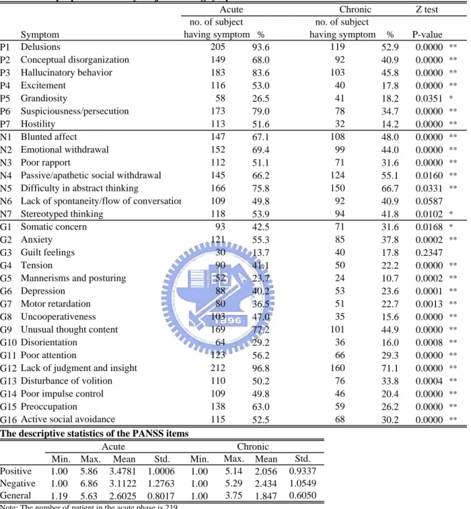
(32) is a small number of basic groups into which cases fall. Briefly, RLCA works as follows: The data required for input consist of the frequencies of all possible cross-classifications of the observed. RLCA then uses maximum likelihood estimation to fit one or a series of hypothesized models to explain covariance patterns among the observed indicators. The parameters of RLCA are: (1) the prevalence of each of J latent classes, which are ηj (xi ) where xi is a P × 1 vector of covariate and j = 1, · · · , J; i = 1, · · · , N , and (2) conditional probabilities for each combination of latent class, item or variable (the items or variables are termed the manifest variables), and response level for the item or variable, which are pmkj where m (= 1, · · · , M ) is the mth items or variables and k (= 1, · · · , Km ) is the kth level of the mth items or variables, that a randomly selected member of that class will make that response to that item/variable. The latent class probabilities provide information about the frequency of occurrence of each latent class. The latent conditional probabilities provide information about the degree of association between each of the observed variables and the latent classes, and are analogous to factor loadings in factor analysis (McCutcheon, 1987). Conditional probabilities give the sensitivity of the observed variables for indicating a particular latent class. Further technical details about parameter estimation and other aspects of RLCA can be found in Huang and Bandeen-Roche (2004). 3.2.5. Analytic Strategy. Table 2 shows the demographic, environmental factor and neuropsychological characteristics description which was done with frequencies and percentages for categorical variables and with means and standard deviations for continuous variables. In the Table 2, it seems that the characteristics of demographic variables of the acute patients were non-different from the chronic patients. A regression extension of latent class analysis (RLCA) was performed on the 30 PANSS-CH, Positive, Negative and General psychosocial scale items to explore the underlying latent structures. The supplement items were not included in this study because the. 21.

(33) ratio of subjects who were assessed on the supplement items was too low, and the majority of researches about explaining the factor structures of the PANSS were using the 30 items to analyze. In addition, because the latent class analysis with 7-point scale is too complex and has large number of parameters, we reduced the 7-point scale on PANSS-CH to the binary scale (no symptom and having symptom) to analyze. Note that no symptom was composed of 1(absent) and 2 (minimal) scales, because the patients who were diagnosed with the minimal scale by psychiatrists had almost no symptom. The frequencies and percentages of the PANSS items and the characteristics of positive, negative and general psychosocial items were shown in Table 3. In the Table 3, the frequencies and percentages of the PANSS items of the acute patients were more than of the chronic patients, except the guilt feelings (G3) item. The means of positive, negative and general symptoms in the acute phase were also more than in the chronic phase. In this study, first, we preformed RLCA without covariates to select number of class by the AIC and BIC criteria to explore the latent structures of PANSS. Second, we preformed RLCA with the demographic variables to explore the correlation between the structures and demographic variables. Third, after looking for the significant demographic variables, we preformed RLCA with environment factors or neuropsychological variables, which were adjusted the significant demographic variables, to explore the correlation between the structures and environment factors or neuropsychological variables. The neuropsychological variables were interrelated, hence we performed RLCA with each one neuropsychological variable specifically. The statistic analysis was used our program (written by R statistical computing software and C program) and Mplus version 3 (Muthén and Muthén, 2004).. 22.

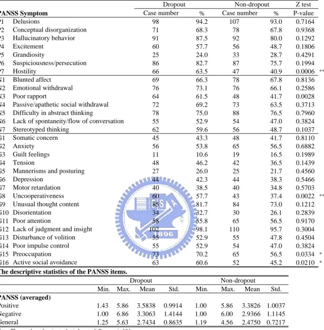
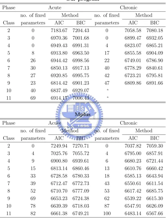
(34) 3.3 3.3.1. Results Selecting the Number of Latent Classes. The literature on the classification of schizophrenic symptomatology included models that use between two and five dimensions to explain the heterogeneity of schizophrenic symptoms. Some of the earlier models were theory-driven, whereas the recent models were based on the results of exploratory factor analysis (EFA). However, factor analysis is used for continuous and usually normally distributed observed variables, where the PANSS items are all categorical. Therefore, we performed latent class analysis (LCA) with number of latent classes varying from two to eleven for selecting the best number of classes by AIC and BIC criteria using our program. We tried different seeds for obtaining various results to find the trend of unstable model. In the present study, the average AIC and BIC values were shown. On the other hand, we used Mplus version 3 to obtain results again to contrast our results. Results of AIC and BIC values for LCA in two phases were shown in Figure 1 and Table 4. Figure 1 shows that, in the acute phase, the AIC and BIC values based on our program both decreased from the two- to five-class, but began to arise at the six-class. However, the AIC and BIC values based on Mplus both decreased from the two- to six-class and began to smooth from the six-class. In the chronic phase, the AIC and BIC values based on our program both decreased from the two- to four-class, but began to arise at the five-class. However, the AIC and BIC values based on Mplus both decreased from the two- to five-class and began to smooth from the five-class. According to the result based on our program, we could select the five- and four- class in the acute and chronic phases, respectively. However, according to the results of Mplus, the chosen numbers of classes in two phases were one class more than our results. Furthermore, we found that in the acute phase, the number of fixed parameters at the six-class model was twice more than that at the five-class model, and in chronic phase, the number of fixed parameters at the four-class. 23.

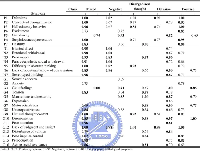
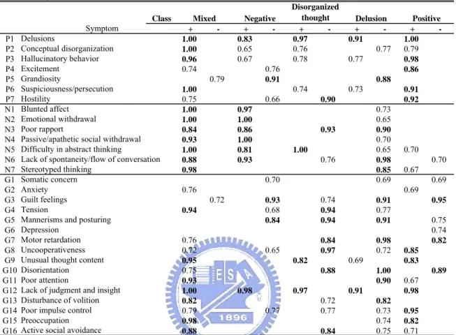
(35) model was also twice more than that at the five-class model. These findings were the same in our results and results of Mplus as shown in Table 4. In addition, the lowest latent prevalence in the six-/five-class model in the acute/chronic phase was under ten percent (Table 5). These results implied that the five-/six-class model with the large number of fixed parameters in the chronic/acute phase were more unstable than the four-/five-class model. In fact, in the previous study, the five factors were generally identified in patients in the acute phase (Bell et al., 1994b), and four or five main factors had been reported in chronic-disease patients (Loas et al., 1997). Therefore, we determined to choose the fiveand four-class in acute and chronic phase, respectively, for further analysis. 3.3.2. Results of the Latent Class Model. The AIC and BIC criteria were suggestive of five- and four-class in the acute and chronic phase. We used latent class regression with the selected number of class to explore the latent structure of PANSS. There are two types of parameters in the latent class model: latent class probabilities and latent conditional probabilities. The results of the two phases were described as follows.. Results of the Acute Phase Table 6 shows that the summarized results of the acute phase with the latent five-class model without covariates which was run by our program. The first class was the mixed class because of high conditional probabilities on the most positive, negative, and general psychopathological items of the PANSS. In the second class, the conditional probabilities of a positive item (P1), six negative items (N1-N6), and a general psychopathological item (G12) were greater than or equal to 0.8. Since the patients of the second class were diagnosed with the most negative symptoms, we labeled it as the negative class. In the third class, there were delusions (P1), conceptual disorganization (P2), hallucinatory behavior (P3), suspiciousness/persecution (P6), difficulty in abstract thinking (N5), unusual thought content (G9) and lack of judgment and insight (G12) with high conditional 24.

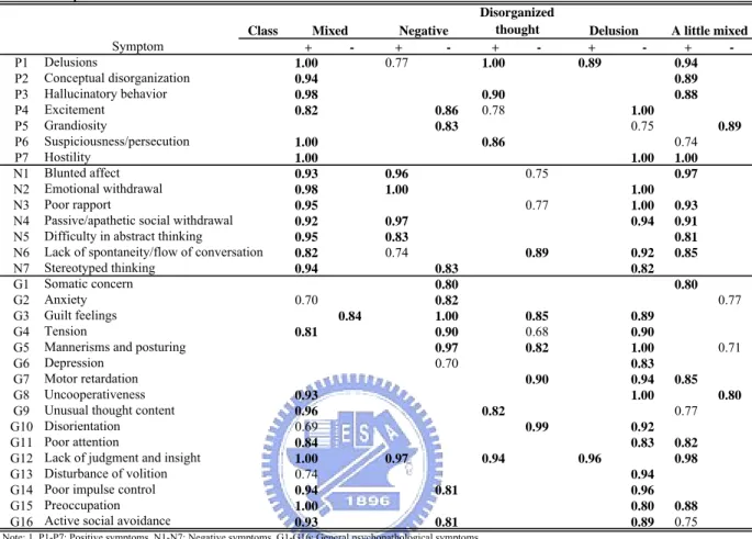
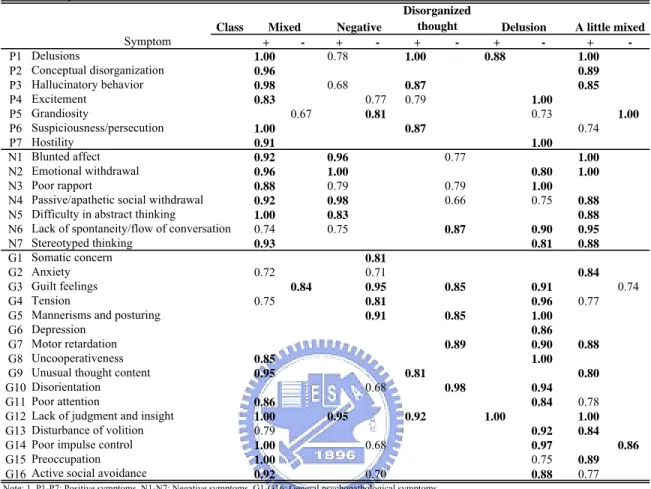
(36) probabilities. These majority symptoms related with thought, therefore the disorganized thought was labeled to the third class. In the fourth class, the patients had the significant symptoms, delusions (P1), hallucinatory behavior (P3), suspiciousness/persecution (P6), unusual thought content (G9) and lack of judgment and insight (G12). Ninety percent of the patients in the fourth class had delusions (P1) symptom, therefore we labeled the fourth class as the delusion class. The fifth class could be labeled as the positive class, because the patients had the likelihood of eighty percent or higher to have six positive items (P1-P4, P6, P7) and the four general psychopathological items (G9, G12, G14, G15). In addition, five latent class probabilities of each class were about equal with the disorganized thought class (the third class) having the lowest prevalence 0.15. In addition, we also performed the latent class model of the acute phase using Mplus version 3, and the results were concluded in Table 7. The first class was similar to the first class of results based on our program, and it was labeled as the mixed class. The second class was also similar to the second class of results based on our program, which had the high conditional probabilities on the blunted affect (N1), emotional withdrawal, passive/apathetic social withdrawal (N4), difficulty in abstract thinking (N5), and lack of judgment and insight (G12). We also labeled the negative class to the second class of resulting from Mplus. In the third class, the conditional probabilities of the delusions (P1), hallucinatory behavior (P3), suspiciousness/persecution (P6), unusual thought content (G9) and lack of judgment and insight (G12) were greater than eighty percent. It was similar to the third class of results based on our program, thus we also labeled it as the disorganized thought. In the fourth class, there were only two significant symptoms, delusions (P1) and lack of judgment and insight (G12). The delusion was labeled to the fourth class, which was similar to the fourth class of resulting from our program. In the fifth class, the conditional probabilities of four positive items (P1-P3, P7), five negative items (N1, N3-N6), and five general psychopathological items (G1, G7, G11, G12, G15) were greater than or equal to eighty percent. The patients of the fifth class were diagnosed 25.

(37) as having several positive, negative and general psychopathological symptoms. However, the number of symptoms diagnosed of the fifth class was less than of the mixed class, thus we labeled it as the a little mixed class. The fifth class resulting from our program was nested within the fifth class resulting from Mplus, where the conditional probabilities of negative items (N1, N3-N6) based on our program were not as significant as the ones based on Mplus. • Demographic Variables We performed the latent class model with demographic variables to explore the relation between the latent class and demographic variables. In Table 8, the summary based on the resulting from our program was demonstrated, whereas the summary resulting from Mplus was shown in Table 9. The symptoms of each latent class were similar to the latent class without covariates. There were also five classes labeled: mixed, negative, disorganized thought, delusion and positive/a little mixed. According to the result based on our program, the parameter estimate of gender in the negative class versus the positive class was significantly different from 0. The parameter estimate was the log odds ratio of having negative symptoms when comparing men with women. The odds ratio for association between gender and having negative symptoms was e0.9 = 2.47. The men were 2.47 times more likely to develop negative symptoms than women. In addition, the older patients would be having serious symptoms, because the log odds ratio of age in the mixed class versus the positive class was significantly different from 0. The patients with fewer years of education were more likely to be in the mixed class or the disorganized thought class because the log odds ratio of years of education in the mixed/disorganized thought class versus the positive class was negative. On the other hand, the odds ratio of years of education in the delusion class versus the positive class was e0.17 = 1.19, thus the patients with high years of education were more likely to develop delusion symptoms. The log odds ratio of occupation in the delusion class versus the positive class was significantly different from 0. The result expressed that the patients 26.

(38) with occupation had high probability to belong to the delusion class. In addition, the patients with the older age at onset would belong to the delusion class, because the odds ratio of age of onset of psychotic symptom in the mixed class versus the positive class was e0.15 = 1.17. According to the conclusion based on Mplus, there was only one significant parameter estimate of gender in the delusion class versus the a little mixed class. The parameter estimate was the log odds ratio of having delusion symptom comparing men with women. The odds ratio for association between gender and having delusion symptoms was e−1.31 = 0.27. The women were 3.71 (=1/0.27) times more likely to develop delusion symptom than men. • Environmental Factors We performed the latent class model with environmental factors after adjusting significant demographic variables to explore the relation between the latent class and environmental factors. The conclusion resulting from our program was shown in Table 10, and the result based on Mplus was shown in Table 11. The symptoms of each latent class were similar to the latent class without covariates. There were also the five classes labeled: mixed, negative, disorganized thought, delusion and positive/a little mixed. Based on the conclusion resulting from our program, after the adjustment of significant demographic variables, i.e., gender, age, years of education, occupation and age of onset of psychotic symptom, the parameter estimate of the slight environmental factor 2 in the negative class versus the positive class was significantly different from 0. The result indicated that patients who had unstable mood or abnormal behavior to interfere with adapting to the daily life had higher tendency to be listed in the negative class than the patients without unstable mood or abnormal behavior, as compared with the positive class. In addition, patients who had no unstable mood or abnormal behavior to interfere with adapting to life had higher trend to be assigned to the mixed class than patients who had these characteristics, as compared with the positive class, because the parame27.

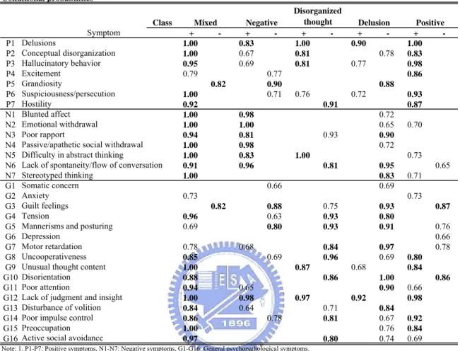
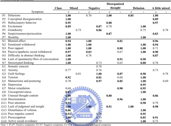
(39) ter estimate of the obvious environmental factor 2 in the mixed class versus the positive class was significant negative. Patients who had obvious psychological problems in their infancy were also more likely to belong to the delusion class than the patients without psychological problems, as compared with the positive class, because the parameter estimate of the obvious environmental factor 3 in the delusion class versus the positive class was significantly different from 0. However, according to the result based on Mplus, after the adjustment of significant demographic variable, i.e., gender, there were no significant parameter estimates of the environmental factors, as shown in Table 10. • Neuropsychological Variables In the acute phase, the neuropsychological variables only contained the sensitivity index (d’) of the CPT performance to reflect the subject’s sustained attention. According to both conclusions based on our program and Mplus, the symptoms of each latent class were similar to the latent class without covariates. According to the result based on the program (Table 12), the undegraded d’ was significant in the negative class versus the positive class. The result elucidated that the patients who had low sustained attention were more likely to be in the negative class than the patients who had high sustained attention, as compared with the positive class. However, the parameter estimates of the undegraded d’ by the latent class model using Mplus were non-significant, as shown in Table 13. In addition, Table 14 and 15 also shows the fact that the parameter estimates of degraded d’ in the resulting from our program or Mplus were non-significant.. Results of the Chronic Phase In Table 16, the summary of the results of the chronic phase with the latent four-class model without covariates which was run by our program was demonstrated. The result based on our program indicated that the first class was labeled as the a little mixed class because of high conditional probabilities on three positive (P1-P3), two negative (N4N5), and two general psychopathological (G9, G12) symptoms. The second class could. 28.

(40) be labeled as a pure negative one, because there were only significant negative symptoms. In the third class, there were only two significant symptoms, delusions (P1) and lack of judgment and insight (G12). We thus labeled the third class as the delusion class. In the fourth class, the patients were diagnosed as being without any symptoms, thus the nosymptoms class was labeled to the fourth class. In addition, the latent class probabilities were equal to or greater than twenty-three percent. In Table 17, the conclusion based on Mplus showed that the symptoms of each latent class were similar to the conclusion resulting from our program. There were also four classes labeled: a little mixed, negative, delusion and no-symptoms. • Demographic Variables The symptoms of each latent class of adding the demographic variables were in common with the results without covariates, as shown in Table 18 and Table 19. The age variables in the a little mixed class versus the no-symptoms class were significant when our program and Mplus were applied. The result indicated that the older patients would have more serious symptoms. In addition, patients with higher years of education would have no symptoms because the log odds ratio of years of education of the conclusion based on our program in the a little mixed/negative/delusion class versus the no-symptoms class was negative. According to the conclusion based on Mplus, the odd ratio of years of education in the a little mixed/negative class versus the no-symptoms class was also negative, thus patients with high years of education were more likely to have no symptoms. In both conclusions based on our program and Mplus, the log odds ratio of occupation in the a little mixed/negative class versus the no-symptoms class was significantly different from 0, representing that the patients without occupation had high probability to belong to the a little mixed/negative class. In addition, the result based on our program also indicated that the single patients would belong to the a little mixed class, because the odds ratio of marital status in the a little mixed class versus the no-symptoms class was e1.39 = 4.03. • Environmental Factors 29.