並聯矩陣沙伯紐式風車效率改善數值研究

(1)

國立交通大學

機械工程學系

碩士論文

並聯矩陣沙伯紐式風車效率改善數值研究

CFD Analysis for the Improvement on Power Efficiency

of Savonius Wind Rotors in Parallel Matrix System

研究生：蘇子博

指導教授：陳俊勳教授

(2)

並聯矩陣沙伯紐式風車效率改善數值研究

CFD Analysis for the Improvement on Power Efficiency of Savonius Wind Rotors in Parallel Matrix System

研究生：蘇子博 Student：Tzu-Po Su 指導教授：陳俊勳 Advisor：Chiun-Hsun Chen 國立交通大學機械工程學系碩士論文 A Thesis

Submitted to Department of Mechanical Engineering College of Engineering

National Chiao Tung University In Partial Fulfillment of the Requirements

For the Degree of Master of Science In Mechanical Engineering

October 2013

Hsinchu, Taiwan, Republic of China

(3)

並聯矩陣沙伯紐式風車效率改善數值研究 學生：蘇子博指導教授 : 陳俊勳國立交通大學機械工程學系

摘要

本研究使用流體力學套裝軟體 Fluent 分析二葉式沙伯紐式風車周圍的流場與其對應的效能。效能的衡量標準為功率係數 Cp(power coefficient)。本研究內容可分為三部分：其一為對單一風車的研究，其二為四風車並聯矩陣系統的研究，其三為十風車並聯矩陣系統的研究。三個系統將會與其分別對應的參數進行研究。在參數分析中，改變參數為風速與周速比，在此之後會探討風向對並聯矩陣系統的影響。最後，本研究將討論三種系統的差異比較。由數值模擬結果顯示，單一風車之最大 Cp值為 0.191，發生在周速比 0.8 的情況下；四風車並聯矩陣系統之最大 Cp值為 0.402，發生在周速比 0.9 的情況下；而十風車並聯矩陣系統之最大 Cp值為 0.438，發生在周速比 0.7 的情況下。十風車並聯矩陣系統的平均 Cp值是單一風車的 2.25 倍，四風車並聯矩陣系統的平均 Cp值是單一風車的 2.07 倍，而十風車並聯矩陣系統的平均 Cp值是四風車並聯矩陣系統的 1.08 倍。三個系統的功率係數（Cp）分別在同一周速比的情況下，會隨風速提升而略微提高。並聯矩陣系統的效能提升主要歸因於風車間的正向干擾情形，而流場的波動現象在此效應中扮演主要角色，但此種正 i

(4)

向干擾效應受風向改變的影響極大。當風向改變為 0°時，其效能幾乎不會改變，甚至低於單一風車情況下的效能。

關鍵字：沙伯紐式風車、並聯矩陣系統、功率係數

(5)

Student: Tzu-Po Su Advisor: Prof. Chiun-Hsun Chen

Department of Mechanical Engineering National Chiao Tung University

ABSTRACT

This study employs a computational fluid dynamics (CFD) software, Fluent, to analyze the flow fields around two-bladed Savonius wind rotors and their corresponding performances. This research includes three cases: the first one is a study of a single Savonius wind rotor, the second is the parallel matrix system, consisting of four two-bladed Savonius wind rotors, and the last one is the parallel matrix system of ten two-bladed Savonius wind rotors. All of the cases are carried out by the corresponding parametric studies, whose parameters include the wind velocity and tip speed ratio. After that, the influence of wind direction change on the parallel system is also studied. Then, comparisons between the systems mentioned above are discussed.

The simulation results show that the maximum Cp value of one

single Savonius wind rotor is 0.191 at tip-speed ratio 0.8; the parallel matrix system with four Savonius wind rotors is 0.402 at tip-speed ratio 0.9; the parallel matrix system with ten Savonius wind rotors is 0.438 at

tip-speed ratio 0.7. The average Cp of the parallel matrix system with ten

Savonius wind rotors is 2.25 times higher than that in one single Savonius

wind rotor and the average Cp of the parallel matrix system with four

(6)

Savonius wind rotors is 2.07 times higher than that in one single Savonius

wind rotor. However, the average Cp of the parallel matrix system with

ten Savonius wind rotors is 1.08 times higher than that in the parallel matrix system with four Savonius wind rotors.

The Cp of these three cases slightly increase with wind speeds at the

same tip speed ratio. The higher performance of parallel matrix system is resulted from the positive interaction between these Savonius wind rotors, and the flow fluctuation plays the major role in contributing to this effect, but this effect is strongly influenced by the change of wind direction.

When wind direction is 0°, the Cp of the parallel matrix system becomes

almost the same or even lower than that of a single one.

Keywords: Savonius wind rotor; parallel matrix system; Cp (power

coefficient)

(7)

ACKNOWLEDGEMENTS

首先必須感謝我的指導教授陳俊勳教授，總是耐心地糾正我的錯誤並給予指導，在老師用心的教誨下，使我在這兩年內學習到許多處理事情與解決問題的能力。感謝曾錦鍊學長給了我這個題目並也給予許多指導。再來是感謝這兩年陪我一起度過的諸位同學們，不論是一同修課或是一同吃飯，不管在瑣事還是正事上都給我許多幫助。這兩年我們一同走過的經歷，這些都歷歷在目。還有實驗室的諸位學長們，在研究中所遇到的問題你們總是不吝指教，也不會在我們面前擺出學長的架子，讓人覺得十分親近。另外也感謝學長馮嘉軒、黃天洋教導我許多風車模擬以及論文寫作的技巧。感謝所有曾經給過我鼓勵的朋友們，雖然可能一時無法把名字都一一點出來，但你們曾經給予過我的，我都不會忘記。最後，鄭重地感謝我的家人，雖然不常在家，但你們總是最默默支持我的一群，這才是我在遇到挫折時還能繼續前進的最大動力。未來還有許多的路要走，大學一路上來，並在研究所這兩年的經歷與學習，實在立定了我人生未來道路的基礎。 v

(8)

LIST OF TABLE

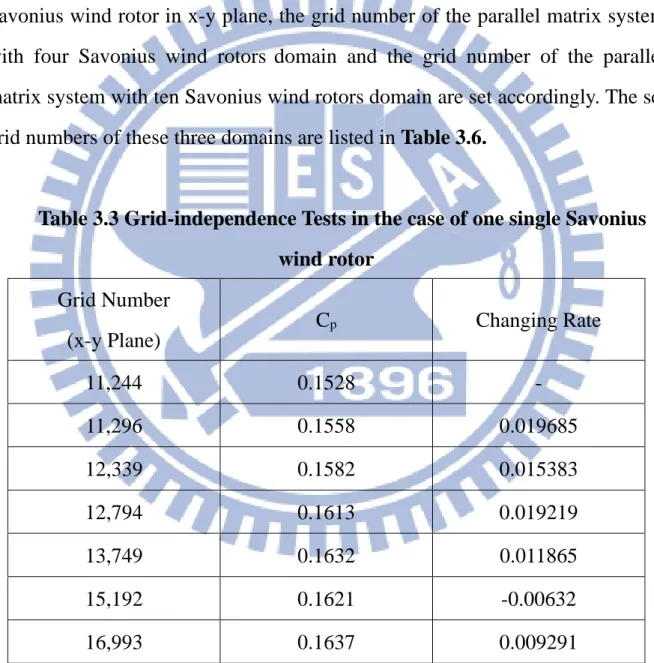
Table 3.1 Geometrical Data ... 24 Table 3.2 Dimensions of Computational Domains ... 25 Table 3.3 Grid-independence Tests in the case of one single Savonius

wind rotor... 43 Table 3.4 Grid-independence Tests in the case of the parallel matrix

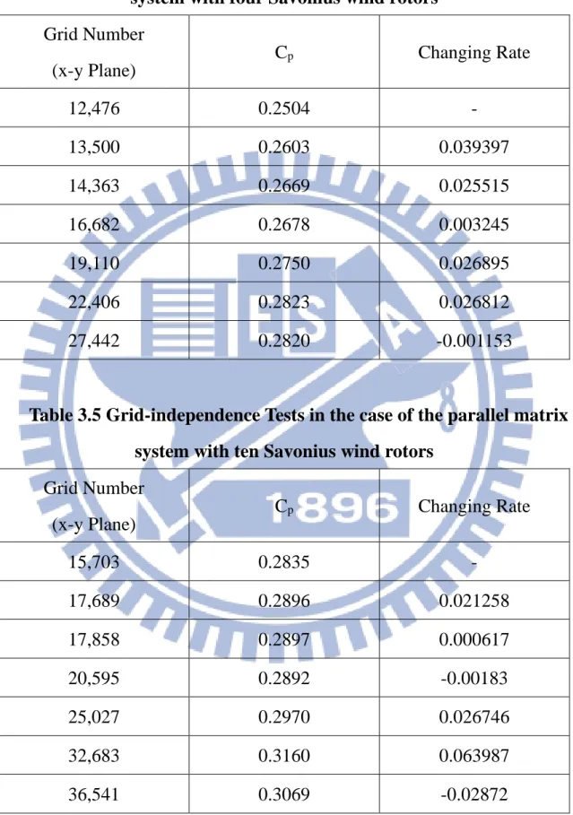
system with four Savonius wind rotors ... 44 Table 3.5 Grid-independence Tests in the case of the parallel matrix

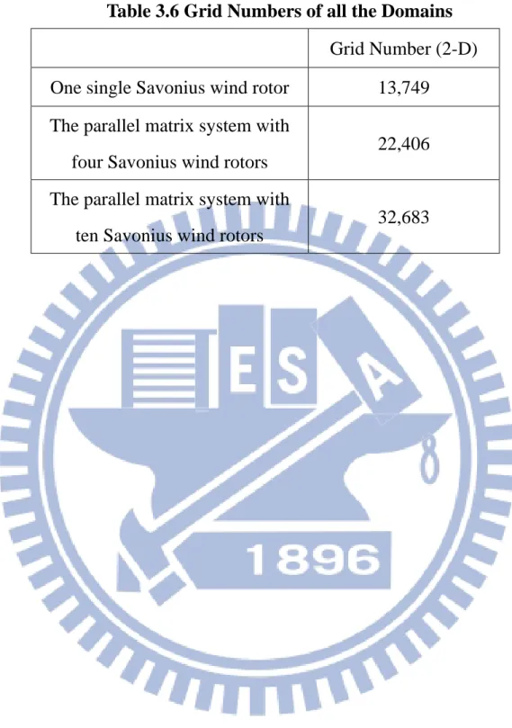
system with ten Savonius wind rotors ... 44 Table 3.6 Grid Numbers of all the Domains ... 45 Table 4.1 Geometry of Savonius wind rotor: present thesis; Feng [1];

Huang [2] ... 54 Table 4.2 Parameters for one single Savonius wind rotor ... 55

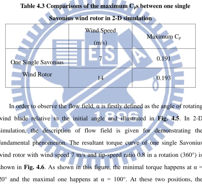
Table 4.3 Comparisons of the maximum Cps between one single Savonius

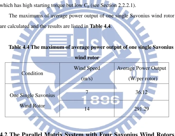
wind rotor in 2-D simulation ... 56 Table 4.4 The maximum of average power output of one single Savonius

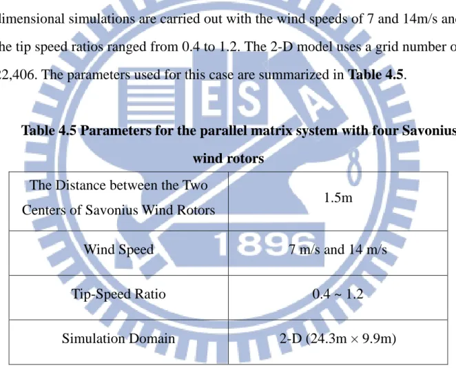
wind rotor... 57 Table 4.5 Parameters for the parallel matrix system with four Savonius

wind rotors ... 58

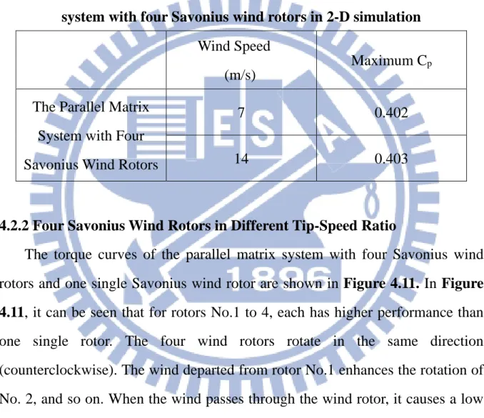
Table 4.6 Comparisons of the maximum Cps between the parallel matrix

system with four Savonius wind rotors in 2-D simulation ... 59 Table 4.7 The maximum of average power output of the parallel matrix

system with four Savonius wind rotors ... 60 Table 4.8 Parameters for the parallel matrix system with ten Savonius

wind rotors ... 61

(12)

Table 4.9 Comparisons of the maximum Cps between the parallel matrix system with ten Savonius wind rotors in 2-D simulation ... 62 Table 4.10 The maximum of average power output of the parallel matrix

system with ten Savonius wind rotors ... 65

Table 4.11 Predicted Cps at different Tip-speed Ratios in 2-D simulations:

(a) one single rotor (b) parallel matrix systems ... 67 Table 4.12 The maximum of average power output of the parallel matrix

systems and one Single Savonius wind rotor ... 69

(13)

LIST OF FIGURES

Fig. 1.1 Global CO2 emissions from fossil fuel burning, 1850 to 2007.

Gas fuel includes flaring of natural gas. All emission estimates

are expressed in Gt CO2 (Boden and Marland, 2010) [19] ... 10

Fig. 1.2 Life cycle CO2 emission factors for different types of power

generation systems [20] ... 10 Fig. 1.3 Structures of wind turbine [21] ... 11 Fig. 1.4 Wake effect from wind turbine picture (Riso National Laboratory,

Denmark) [22] ... 11 Fig. 1.5 Schematic of a two-bladed Savonius wind rotor [4] ... 12 Fig. 1.6 Streamlines around three Savonius wind rotors with phase angle

90° difference. [1] ... 12 Fig. 1.7 The scope of this study ... 13 Fig. 2.1 Idealized fluid model for a wind rotor [23] ... 22

Fig. 2.2 Characteristic curves of CP averaged as a function ofλfor various

wind turbines. [17] ... 22 Fig. 2.3 Flow conditions and aerodynamic forces with a drag device [24] ... 23 Fig. 2.4 Aerodynamic forces acting on an airfoil exposed to an air stream

[24] ... 23 Fig. 3.1 Schematics of Savonius wind rotor geometry in experimental

study ... 46 Fig. 3.2 The domain of one single Savonius wind rotor ... 46 Fig. 3.3 The domain of four two-bladed Savonius wind rotors in parallel

matrix system ... 47

(14)

Fig. 3.4 The domain of ten two-bladed Savonius wind rotors in parallel

matrix system ... 47

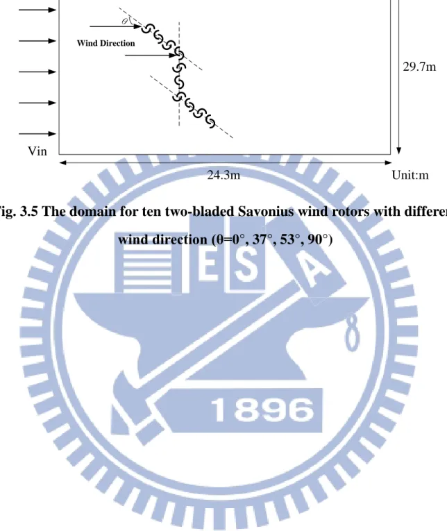
Fig. 3.5 The domain for ten two-bladed Savonius wind rotors with different wind direction (θ=0°, 37°, 53°, 90°) ... 48

Fig. 3.6 Overview of the segregated solution method ... 49

Fig. 3.7 Control volume used to illustrate discretization of a scalar transport equation ... 49

Fig. 3.8 Zones created by non-periodic interface intersection ... 50

Fig. 3.9 Two-dimensional grid interface ... 50

Fig. 3.10 User interface of Gambit ... 51

Fig. 3.11 Grid-independence tests: (a) one single Savonius wind rotor; (b) the parallel matrix system with four Savonius wind rotors; (c) the parallel matrix system with ten Savonius wind rotors ... 52

Fig. 4.1 Schematics of Savonius wind rotor geometry: (a) present thesis; (b) Feng [1]; (c) Huang [2] ... 71

Fig. 4.2 The 2D simulation of one single Savonius wind rotor comparing with Feng’s predictions [1], Huang’s predictions [2] and experimental measurements by Howell et al. [12] in: (a) wind speed 7 m/s; (b) wind speed 14 m/s... 72

Fig. 4.3 The performance of one single Savonius wind rotor ... 73

Fig. 4.4 Velocity vector distribution around one single Savonius wind rotor at α=100° in wind speed: (a) 7m/s; (b) 14m/s ... 74

Fig. 4.5 The defined angle α of rotating wind blade relative to the initial angle ... 74

Fig 4.6 Torque curve of one single Savonius wind rotor with wind speed 7 m/s and tip-speed ratio 0.8 in a rotation ... 75

(15)

Fig. 4.7 Static pressure field around one single Savonius wind rotor in

2-D simulation at: (a) α=20°; (b) α=100° ... 76

Fig. 4.8 Velocity vector distribution around one single Savonius wind

rotor in 2-D simulation at: (a) α=20°; (b) α=100° ... 77

Fig. 4.9 Phase-averaged pressure difference from the average pressure field [14] ... 77 Fig. 4.10 Velocity vector distribution around the parallel matrix system

with four Savonius wind rotors in wind speed: (a) 7m/s; (b) 14m/s ... 78 Fig. 4.11 Torque curves of the parallel matrix system with four Savonius

wind rotors and one single Savonius wind rotor ... 79 Fig. 4.12 Static pressure field around the parallel matrix system with four

Savonius wind rotors ... 79 Fig. 4.13 Velocity vector distribution around the parallel matrix system

with four Savonius wind rotors ... 80 Fig. 4.14 Streamlines around the parallel matrix system with four

Savonius wind rotors at wind speed 7 m/s and TSR 0.9 ... 80 Fig. 4.15 Comparison of the parallel matrix system with four Savonius

wind rotors and one single Savonius wind rotor ... 81 Fig. 4.16 Velocity vector distribution around the parallel matrix system

with ten Savonius wind rotors in wind speed: (a) 7m/s; (b) 14m/s ... 82 Fig. 4.17 Torque curves of the parallel matrix system with ten Savonius

wind rotors and one single Savonius wind rotor ... 82 Fig. 4.18 Static pressure field around the parallel matrix system with ten

Savonius wind rotors ... 83

(16)

Fig. 4.19 Velocity vector distribution around the parallel matrix system with ten Savonius wind rotors ... 83 Fig. 4.20 Streamlines around the parallel matrix system with ten Savonius

wind rotors at wind speed 7 m/s and TSR 0.7 ... 84 Fig. 4.21 Comparison of the parallel matrix system with ten Savonius

wind rotors and one single Savonius wind rotor ... 84 Fig. 4.22 Three-rotor with phase angle difference 90° in different wind

directions [1] ... 85 Fig. 4.23 the parallel matrix system with ten Savonius wind rotors in

different wind directions ... 85 Fig. 4.24 Velocity vector distribution around the ten Savonius wind rotors

with a change of wind direction θ (a) θ = 0°; (b) θ = 37°; (c) θ = 53°; (d) θ = 90° ... 87 Fig. 4.25 Static pressure field around the ten Savonius wind rotors with a

change of wind direction θ (a) θ = 0°; (b) θ = 37°; (c) θ = 53°; (d) θ = 90° ... 89

Fig. 4.26 Predicted Cps at different Tip-speed Ratios in 2-D simulations:

(a) one single rotor; (b) parallel matrix system ... 90 Fig. 4.27 Comparison of the parallel matrix system with ten Savonius

wind rotors, the parallel matrix system with four Savonius wind rotors and one single Savonius wind rotor ... 91

(17)

CHAPTER 1 INTRODUCTION

1.1 Motivation

The fossil fuel resources on earth are limited, and the global demands for gas, oil and coal exceed the supplies. As a consequence, they are more and more expensive. Therefore, the heavily dependence on fossil fuels could cause serious problems, including energy shortage and carbon dioxide emissions due to burning of fossil fuels.

As shown in Fig. 1.1, Carbon dioxide emissions are increasing year by year that cause global warming. Hence, researches of renewable energy are extremely important. Many countries are committed to develop the renewable energies,

such as wind energy, solar energy, geothermalenergy, ocean energy, hydropower

and bioenergy. The carbon dioxide emissions are very low during the production processes of these renewable energy sources, as illustrated in Fig. 1.2. Although nuclear power does not emit any carbon dioxide during power generation, but there are strong oppositions against strengthening nuclear power in many countries of the world due to its safety and waste-handling problems. As mentioned previously, wind energy is one of the important renewable energies, which has a much lower carbon dioxide emission compared with the fossil fuel resources. In other words, its pollution to the environment is very low.

Wind power is the conversion of the wind momentum energy into a useful form of energy. There are two kinds of principal wind turbine designs. They are horizontal-axis wind turbines (HAWTs), whose rotation axis is parallel to the

(18)

horizon, and vertical-axis wind turbines (VATWs), whose axis is perpendicular to the horizon. Their structures are demonstrated in Fig. 1.3. It is commonly

known that the power coefficient (Cp) of HAWTs, ranged from about 0.30 to

0.45, is higher than that of VAWTs, whose range is from 0.15 to 0.30. However, there are a few problems in HAWTs. First, HAWTs spinning with high tip speed ratio always cause the low-frequency sound to make noise pollution. Second, it is necessary to need a sufficient distance between the wind rotors in order to avoid wake effect (see Fig. 1.4), resulting in a lower energy conversion. Third, the fan should be aligned with the wind direction in order to obtain a better efficiency, but it always takes a long time to adjust. Last but not the least, the costs of land preparations, installation, maintenance and repair of HAWTs are considerable. On the other hand, VAWTs, with the low-cost capital and simple structure, can be more efficiently installed in the low wind area. It can be divided into two categories based on their blade designs: Darrieus wind turbine is lift-type, whereas Savonius wind turbine is drag-type. Relative to the

drag-type wind turbines, the lift-type wind turbine has a better value of Cp, but

the starting torque is low. Besides, Savonius wind turbine is noiseless and it is able to bear the wind with fluctuation. However, the power efficiency needs to be improved.

Even though the Cp of HAWTs is higher than the one of VAWTs, there are a

lot of methods to improve the latter one’s performance. In order to achieve this purpose, for instance, it can put a series of VAWTs connecting in parallel with a fixed distance between them, and they rotate with a specific phase angle difference. In Feng’s preliminary study [1], the simulation of parallel matrix system consisted of three two-bladed Savonius wind rotors, as shown in Fig. 1.5,

to rotate with 90 degree phase angle deference. Its Cp is about 1.45 times that of

(19)

one single Savonius wind rotor in 3-D simulation. Following by Huang’s study [2], the simulation of parallel matrix system adopted four two-bladed Savonius

wind rotors to rotate with 90 degree phase angle deference (see Fig. 1.6). Its

average Cp is about 1.46. To further enhance the efficiency of two-bladed

Savonius wind rotor parallel matrix system, the present work intends to establish three groups of four two-bladed Savonius wind rotors parallel matrix systems and investigating their respective performance by using computational fluid

dynamics (CFD) technique. And then find the optimum Cp value. In this way,

the best performance can be expected to find by fully utilizing wind fields in effect.

1.2 Literature Review

The Savonius wind rotor is a drag-typed vertical-axis wind rotor, developed by S. J. Savonius [3]. Its shape is similar to the character “S”, therefore, it is also called S-rotor. This kind of rotor is spinned by drag force. The drag force difference between concave and convex surfaces drives the rotor, leading to a large starting torque with a relatively low rotational speed. Many improving researches are bringing up after the Savonius’ development.

Blackwell et al. [4] investigated the performances of fifteen configurations of Savonius wind rotors by testing in a low speed wind tunnel. What they investigated included parameters, such as number of blades, wind velocity, wind rotor height, and blade overlap ratio. The results showed that the two-bladed configurations have better performance than the three-bladed ones, except the starting torque. Besides, the performance increases with aspect ratio slightly, and the optimum overlap ratio is between 0.1 and 0.15.

(20)

Fujisawa [5] studied the performances of two-bladed Savonius wind rotors with different overlap ratios ranged from 0 to 0.5 by experimental investigations. The results reveal that the performance of Savonius wind rotor reaches a maximum value at an overlap ratio of 0.15. It is due to the fact that the flow through the overlap strengthens the forward movement. However, when the overlap ratio becomes larger, the recirculation zone grows accordingly, causing the performance deterioration.

Gupta et al. [6] studied the performances of a Savonius wind rotor and a Savonius-Darrieus machine with overlap variation by experimental investigations. For the Savonius-Darrieus machine, there was a two-bladed Savonius wind rotor in the upper part and a Darrieus machine in the lower side.

The result showed that Cp with 20% overlap is higher than 16.2% without

overlap. They also concluded that the improvement of Cp can be achieved for

the Savonius-Darrieus wind machine compared with the general Savonius rotor.

Irabu and Roy [7] introduced a guide-box tunnel to improve the Cp of

Savonius wind rotors and prevent the damage by strong wind disaster. The guide-box tunnel was like a rectangular box as wind passage and the test wind rotor was included. It was able to adjust the inlet mass flow rate by its variable area ratio between the inlet and outlet. The experimental results showed that the

maximum Cp of the two-bladed wind rotor using the guide-box tunnel is about

1.23 times of that the wind rotor without the guide-box tunnel and 1.5 times of that using a three-bladed wind rotor. Apparently, it verified that the two-bladed wind rotor is better than the three-bladed one for converting wind power.

Saha et al. [8] used a wind tunnel to test and investigate the performances by different number of blades and stages, different geometries of blade and inserting valves on the concave side of blade or not. The results were as follows.

(21)

First, with an increases of the number of blades, the performance of wind rotor decreases. Second, twisted geometry blade profile has a better performance than

the semicircular blade geometry. Third, the Cp of a two-stage Savonius wind

rotor is higher than those of single-stage and three-stage wind rotors. Last, the valve-aided Savonius wind rotor with three blades shows a better performance than the conventional wind rotor.

Altan et al. [9] introduced a curtaining arrangement to improve the performance and increase the efficiency of a two-bladed Savonius wind rotor without changing its basic structure. They placed two wind-deflecting plates in front of the wind rotor to prevent the negative torque opposite the wind rotor

rotation. The experimental results showed that Cp increase about 38% with an

optimum curtain arrangement and it is 16% much higher than that without curtaining.

Antheaume et al. [10] applied the CFD software, Fluent, to investigate the performance of vertical axis Darrieus wind rotor in different working fluids by

using k-ε turbulent model under steady-state conditions. They also discussed the

average efficiency of several wind rotors connected in parallel pattern. The results showed that increasing the number of wind rotors or decreasing the distance between wind rotors can make the efficiency higher due to the velocity streamlines straightening effect by the configuration. In addition, the performances working in water are much higher than those in air.

Zhao et al. [11] applied the computational fluid dynamics (CFD) software to investigate the performance of new helical Savonius wind rotors. They analyzed the behaviors of the wind rotors with different aspects ratio, number of blades, overlap distance and helical angle. The results showed that three-blade

helical wind rotor has lower Cp compared with two-bladed helical wind rotor.

(22)

And the best overlap ratio, aspect ratio, and helical angle are 0.3, 6.0 and 180°, respectively.

Howell et al. [12] applied Fluent to investigate the performances of one VAWT in 2-D and 3-D simulations and compared the predictions with

experimental data. The turbulence model used was RNG k-ε model, by which

the applicability in flow fields involves large flow separations. The error bars on experimental data were fixed at ±20% of measured values. The results showed that the performances predicted by 2-D simulations are apparently higher than those by 3-D simulations and experimental measurements due to the effect of the generation of over tip vortices.

Pope et al. [13] applied Fluent to investigate the performances of zephyr VAWT and compared the predictions with experimental data. By the reason that a free spinning turbine cannot be fully simulated, they used constant rotational speeds of the VAWT in simulations and changed the specification of parameters to reveal freely moving turbine blades in experiments. They indicated that determining the performance at constant rotational speed is valuable since any power generation connected to the electricity grid needs to operate at constant speed.

Shigetomi et al. [14] studied the interactive flow field around two Savonius wind rotors by experimental investigation using particle image velocimetry. They found that there exist power-improvement interactions between two rotating Savonius rotors in appropriate arrangements. The interactions are caused by the Magnus effect to provide the additional rotation of the downstream rotor and the periodic coupling of local flow between two wind rotors. However, they are quite sensitive between two wind rotors to the wind direction so that wind rotors arranged together will lose one of the VAWTs inherent advantages, such as

(23)

no influence of wind direction.

Akwa et al. [15] investigated the influence of the buckets overlap ratio of a Savonius wind rotor on the averaged moment and power coefficients in the complete cycles of operation by the commercial software, Star-CCMþ. Numerical simulations of the air flow on the rotor in 40 different situations were carried out. The results showed that the best performance occurs at bucket overlap ratios with values close to 0.15, giving an averaged power coefficient of 0.3161 under the tip speed ratio 1.25. However, in the range of high bucket overlap, the moment and performance of the rotor fall dramatically due to the reduced incidence of air on the concave side of the rotor bucket.

McTavish et al. [16] studied a performance assessment of a novel vertical axis wind turbine by using CFD software, CFdesign 2010. A validation study consisting of steady and rotating simulations was conducted using a Savonius rotor. Fair agreement was obtained by comparing with experimental data. Steady two-dimensional CFD simulations had demonstrated that the new VAWT has the similar average static torque characteristics to existing Savonius rotors. Three-dimensional simulations were conducted at several tip speed ratios with a free stream speed of 6 m/s. The predicted dynamic torque generated by the rotor decays more rapidly with increasing tip speed ratio than the torque output of Savonius rotors due to its asymmetric design and the curvature of the outer rotor wall.

Akwa et al. [17] presented a review on the performance of Savonius wind turbines. Simple construction, high start up and full operation moment, wind acceptance from any direction, low noise and angular velocity in operation, reducing wear on moving parts, are some advantages of using this type of machine. Savonius rotor performance is affected by operational conditions,

(24)

geometric and air flow parameters. Each different arrangement of Savonius rotor affects its performance. The range of reported values for maximum averaged power coefficient includes values around 0.05–0.30 for most settings. Performance gains of up to 50% for tip speed ratio of maximum averaged power coefficient are also reported with the use of stators.

Zhou et al. [18] explored the non-linear two-dimensional unsteady flow over a conventional Savonius-type rotor and a Bach-type rotor, and developed a simulation method for predicting their aerodynamic performance. The simulations were performed using Star-CCMþ. A comparative study of the two types of rotors was carried out, and numerical simulation results were compared with experimental data. The results showed that the Bach-type rotor is demonstrated to have better performance for torque and power coefficient than the conventional Savonius-type rotor. A discussion of the causes of these differences was presented that is based on a detailed study of the respective flow field characteristics, including the behavior of moment coefficients, velocity vectors and pressure distribution. A simulation method for further study of new blades shapes was suggested.

Feng [1] applied the computational fluid dynamics (CFD) software, Star-CD, to investigate the flow field around two-bladed Savonius wind rotors and their corresponding performances. The study mentioned that using the parallel matrix arrangement of Savonius wind rotors can get higher power efficiency. It

indicated that the parallel matrix system has an optimum Cp, which is about 1.45

times of Cp of one single Savonius wind rotor in 3-D simulation.

Huang [2] applied the CFD software, Fluent, to investigate a four two-bladed Savonius wind rotors in parallel matrix system and compared the

predicted results with experimental data. For the simulation results, the Cp of

(25)

parallel matrix system with curtain is about 1.03 times of that of the system

without curtain. Both of those are occurred at TSR 0.8. Besides, The Cp of

parallel matrix system with curtain at TSR 0.6 is about 1.16 times of that of the system without curtain. However, the predicted results are higher than the

experiment measurements because the resultant Cps in experiments by the

generated power, which needs to consider energy transform loss.

1.3 Scope of Present Study

This study employs a computational fluid dynamics (CFD) software, Fluent, to analyze the flow fields around two-bladed Savonius wind rotors and their corresponding performances. This research includes three cases: the first one is a study of a single Savonius wind rotor, the second is the parallel matrix system, consisting of four two-bladed Savonius wind rotors, and the last one is the parallel matrix system of ten two-bladed Savonius wind rotors. All of the cases are carried out by the corresponding parametric studies, whose parameters include the wind velocity and tip speed ratio. After that, the influence of wind direction change on the parallel system is also studied. Then, comparisons between the systems mentioned above are discussed.

(26)

Fig. 1.1 Global CO2 emissions from fossil fuel burning, 1850 to 2007. Gas

fuel includes flaring of natural gas. All emission estimates are expressed in Gt CO2 (Boden and Marland, 2010) [19]

Fig. 1.2 Life cycle CO2 emission factors for different types of power

generation systems [20]

(27)

Fig. 1.3 Structures of wind turbine [21]

Fig. 1.4 Wake effect from wind turbine picture (Riso National Laboratory, Denmark) [22]

(28)

Fig. 1.5 Schematic of a two-bladed Savonius wind rotor [4]

Fig. 1.6 Streamlines around three Savonius wind rotors with phase angle 90° difference. [1]

(29)

Fig. 1.7 The scope of this study

(30)

CHAPTER 2 FUNDAMENTALS OF WIND ENERGY

2.1 Brief History of Wind Energy

The wind energy has been used for thousands of years such as sailing, grinding grains, irrigation and drawing water. The first windmill appeared in Europe can be traced back to the twelfth century. The first wind machine was known as appearing about 2200 years ago in Persia for grinding grains. Then the Romans used the same way for the same purpose around 250 A.D. By the fourteenth century, the Dutch employed windmills to drain water in the low-lying areas of the Rhine River delta. After many years developing, the Netherlands used windmill to drain wetlands from the fourteenth century onwards and become an economy developed country gradually. Professor James Blyth built an experiment of windmill to produce electricity in Scotland in July 1887. The first use of windmill for producing electricity was in 1888. And the first such windmill was built and used by Charles Brush in Ohio, U.S.A. Ten years later, about 72 wind turbines were being used to produce electricity in the range of about 5 to 25kW.

In the twentieth century, wind turbines were used around the world. Because the first wind power station was established in Denmark in 1891, wind power became an important part of a decentralized electrification in the first quarter of the twentieth century. There existed many small electricity generating sites in Denmark, and wind power was a large part of them. In Australia, small wind generators were used to provide power at isolated post offices and farms. In

(31)

America, rural farms had used wind power originally. Eventually, this generated electricity was connected to grid later. By 1930, windmill had been widely manufactured and used to generate electricity for the distribution system having not yet been installed in America. More than six million wind turbines had been manufactured in American and it was the first time that the utilization of wind energy was based on an industrially mass-produced. Following these experience, American manufacturers started build and sell small wind turbines not only for battery-charging but also for interconnection to electricity networks. The first megawatt wind turbine was built in USA in 1941. In the 1970s and 1980s, the U.S. government promoted the technologies for the large-scale commercial wind turbines. NASA researched many of the turbine designs under this project that still is used today.

In the end of 2002, there was roughly 32 GW of power supplied from wind energy in the world. Europe has been the leader in wind power utilization, contributing 76% of the total. In 2006, roughly 65GW of rated power were installed in wind farms worldwide, of which more than 47GW located in Europe, and more than 11GW in the United States.

2.2 Basic of Wind Energy Conversion

2.2.1 Power Conversion and Power Coefficient

From the expression for kinetic energy in flowing air, the power contained

in the wind passing an area A with the wind velocity v1 is:

𝑃𝑃𝑊𝑊 = 𝜌𝜌₂𝐴𝐴𝐴𝐴13 (2-1)

where ρ is air density, depending on air pressure and moisture. For practical

calculations it may be assumed ρ ≈ 1.225kg/m3. The air streams in axial

(32)

direction through the wind turbine, of which A is the swept area. The useful mechanical power obtainment is expressed by means of the power coefficient

Cp:

𝑃𝑃 = 𝐶𝐶𝑝𝑝𝜌𝜌₂𝐴𝐴𝐴𝐴13 (2-2)

Supposing the wind velocity of airflow is homogeneous, the value ahead of

the turbine plane is v1. After passing through the retardation of wind turbine,

suffers retardation due to the power conversion to a speed v3 far behind the wind

turbine. Due to the power conversion, wind velocity v1 reduce to a velocity v3, as

shown in Fig. 2.1, a simplified theory could be claimed that the velocity can be

represented in an average value v2, where v2 = (v1+v3)/2, in the retardation

where the moving blades located. On this basis, Betz has shown by a simple

calculation that the maximum useful power can be obtained for v3/v1 = 1/3 in

1920; where the power coefficient Cp = 16/27 ≈ 0.593. In reality, wind turbine

displays the maximum values Cp, max = 0.4 ~ 0.5 due to losses, such as profile

loss, tip loss and loss due to wake rotation. In order to determine the mechanical power available for the load machine, such as electrical generator or pump, Eq. (2-2) has to be multiplied with an efficiency of the drive train, taking losses in bearings, couplings and gear boxes into account.

An important parameter of wind rotor is the tip-speed ratio (TSR), λ. It is

defined as a ratio of the circumferential velocity of blade tips to the wind speed: 𝜆𝜆 = 𝑢𝑢 𝐴𝐴� =1

𝐷𝐷 2 ∙

𝜔𝜔

𝑣𝑣1 (2-3)

where D is the outer turbine diameter and ω the angular wind rotor

speed. Considering that in the rotating mechanical system, the power is the

product of torque T and angular speed ω (P = T • ω), then Cp becomes

𝐶𝐶𝑝𝑝 =_𝑃𝑃𝑃𝑃_𝑊𝑊 = 1𝑇𝑇⋅𝜔𝜔 2𝜌𝜌𝐴𝐴𝑣𝑣13

(2-4)

(33)

Fig. 2.2 shows typical characteristics Cp (λ) for different types of wind

rotors. Besides the constant maximum value according to Betz, as well as the

figure indicates a revised curve Cp by Schmitz, who takes the downstream

deviation from axial air flow direction into account. The difference is notable in the region of lower tip speed ratios.

2.2.2 Wind Rotor Blades Using Aerodynamic Drag or Lift

Extract the airflow power to mechanical power without considering design of wind rotor blades. The momentum theory by Betz indicates the physically based, ideal limit value for the extraction of mechanical power from free-stream airflow without considering the design of the energy converter. However, the power which can be achieved under real conditions cannot be independent of the characteristics of the energy converter. The fundamental difference for various rotor blade designs depends on what kind aerodynamic force is utilized to produce the mechanical power. The first fundamental difference which considerably influences the actual power depends on which aerodynamic forces are utilized for producing mechanical power. As the wind rotor blades are subjected to airflow, the generated aerodynamic drag is parallel to the flow direction, whereas the lift is perpendicular to flow direction. The real power coefficients obtained are greatly dependent on whether aerodynamic drag or aerodynamic lift is used.

2.2.2.1 Drag Devices

The simplest type of wind energy conversion can be achieved by means of pure drag surfaces as shown in Fig. 2.3. The air impinges on the surface A with

wind velocity v, and then the drag D can be calculated from the air density ρ, the

(34)

surface area A, the wind velocity u and the aerodynamic drag coefficient CD as

𝐷𝐷 = 𝐶𝐶𝐷𝐷1₂𝜌𝜌𝐴𝐴𝐴𝐴𝑟𝑟2 = 𝐶𝐶𝐷𝐷1₂𝜌𝜌𝐴𝐴(𝐴𝐴 − 𝑢𝑢)2 (2-5)

The relative velocity, vr = v – u, which effectively impinges on the drag area, is

determined by wind velocity v and blade rotating speed u = ωRM, in which RM

is the mean radius. Then the resultant power is

𝑃𝑃 = 𝐷𝐷 ⋅ 𝑢𝑢 = 1₂𝜌𝜌𝐴𝐴𝐴𝐴3�𝐶𝐶𝐷𝐷�1 −𝑢𝑢_𝑣𝑣�2 𝑢𝑢_𝑣𝑣� =1₂𝜌𝜌𝐴𝐴𝐴𝐴3𝐶𝐶𝑝𝑝 (2-6)

Analog to the approach described in Chapter 2.2.1, it can be shown that Cp reaches a maximum value with a velocity ratio of u/v = 1/3. The maximum

value of Cp is then

𝐶𝐶𝑝𝑝,𝑚𝑚𝑚𝑚𝑚𝑚 =₂₇4 𝐶𝐶𝐷𝐷 (2-7)

It is taken into account that the aerodynamic drag coefficient CD of a

concave surface curved against the wind direction can hardly exceed a value of

1.3. Thus, the maximum power coefficient Cp, max of a general drag-type wind

rotor becomes about 0.2, only one third of Betz’s ideal Cp value of 0.593.

2.2.2.2 Lift Devices

Utilization of aerodynamic lift on wind rotor blade can achieve much higher power coefficients. The lift blade design employs the same principle that enables airplanes to fly. As shown in Fig. 2.4, when air flows over the blade, a pressure gradient creates between the upper and the lower blade surfaces. The pressure at the lower surface is greater than upper surface. Thus, the difference of pressure produces a lift force to uplift the blade. The lift force occurred on a body by

wind can be calculated from the air density ρ, acting area A, wind velocity v and

aerodynamic lift coefficient CL as

(35)

𝐿𝐿 = 𝐶𝐶𝐿𝐿1₂𝜌𝜌𝐴𝐴𝐴𝐴2 (2-8)

When blades are attached to the central axis of a wind rotor, the lift force is translated into rotational motion. All of the modern wind rotor types are designed for utilizing this effect, and the best type suited for this purpose is with a horizontal rotational axis. The aerodynamic force created is divided into a component in the direction of free-stream velocity, the drag force D, and a component perpendicular to the free-stream velocity, the lift force L. The lift

force L can be further divided into a component Ltorque in the plane of rotation of

the wind rotor, and a component Lthrust perpendicular to the plane of rotation.

Ltorque constitutes the driving torque of the wind rotor.

Modern airfoils, developed for aircraft wings and which are also applied in wind rotors, have an extremely favorable lift-to-drag ratio. It could show a qualitative utilization of how much an aerodynamic lift force uses as a driving force would have more efficiency. However, it is no longer possible to calculate the power coefficients of lift-type wind rotors quantitatively with the aid of elementary physical relationships alone.

2.3 Vertical and Horizontal Axis Wind Rotors

Wind rotors are approximately classified into two general types by their orientations: horizontal axis type and vertical axis type. A horizontal axis wind rotor has its blades rotating on an axis parallel to the ground and a vertical axis one has its blades rotating on an axis perpendicular to the ground. There are a number of designs for both, and each type has certain advantages and disadvantages. There are numerous designs for both type rotors with different concerns, which are related to diverse situations. Generally, the number of

(36)

vertical axis wind rotor for commercial uses is much less than that of horizontal axis wind rotor.

2.3.1 Wind Rotors with a Vertical Axis of Rotation

The oldest design of wind rotors is fabricated in vertical axis of rotation. At the beginning, vertical-axis wind rotors could only be built for using aerodynamic drag. It was only recently that engineers succeeded in developing vertical-axis designs which could also utilize aerodynamic lift effectively. Darrieus proposed such design, considered as a promising concept for modern wind turbines in 1925. The Darrieus wind rotor resembles a gigantic eggbeater and the geometric shape of the wind rotors blades is complicated that is difficult to manufacture. A wind rotor, called H-rotor, also utilizes aerodynamic lift force. Instead of curved wind rotor blades, the straight blades are connected to the wind rotor shaft by struts.

Furthermore, Savonius wind rotor, which is investigated in this research, is also one type of vertical-axis wind rotors. The wind rotor was invented by a Finnish engineer, Savonius in 1922. The structure of Savonius wind rotor is simple with a shape of character “S”, so it is also called S-rotor. Savonius wind rotor is one of the simplest wind rotors to manufacture. Because it is a drag-typed device, Savonius wind rotor extracts much less wind energy than the other similarly-sized lift-type wind rotor, but it has higher starting torque.

2.3.2 Horizontal Axis Wind Rotors

The earliest design of this type of wind turbine was the big Dutch-style windmill, primarily used for milling grain. Another early type of these turbines was the windmill that was built on almost all farms in the early twentieth century.

(37)

This type of wind turbines is the dominant design principle in wind energy technology today. The undisputed superiority of this design to date is primarily based on the reason that the wind rotor blade shape can be aerodynamically optimized and the highest efficiency can be achieved when aerodynamic lift is utilized appropriately.

These turbines usually need to adjust the angle of the entire wind rotor with the change of wind direction. They achieve the objective by using a yaw system which can move the entire wind rotor left or right in small increments. They can also control the wind rotor torque and power output by adjusting the blade angle using the pitching mechanism. However, designs differing from standard concept are also common and simplifications of construction, such as the absence of the pitching mechanism, can be found, particularly in small wind turbines.

(38)

Fig. 2.1 Idealized fluid model for a wind rotor [23]

Fig. 2.2 Characteristic curves of CP averaged as a function ofλfor various

wind turbines. [17]

(39)

Fig. 2.3 Flow conditions and aerodynamic forces with a drag device [24]

Fig. 2.4 Aerodynamic forces acting on an airfoil exposed to an air stream [24]

(40)

CHAPTER 3 MATHEMATICAL MODEL AND NUMERICAL

ALGORITHM

3.1 Domain Description

In this work, the air flow fields around a single rotating Savonius wind rotor, the parallel matrix system with four Savonius wind rotors and the parallel matrix system with ten Savonius wind rotors are analyzed numerically under different tip-speed ratios by employing Fluent. The geometry of a two-bladed Savonius wind rotor was given in Fig. 1.5 and the corresponding information is summarized in Table 3.1. And, the geometry of real wind rotor is shown in Fig.

3.1.

Table 3.1 Geometrical Data

Number of Blades 2

Rotor Blade Diameter (m) 0.9

Overlap Ratio of Blades 0.15

In order to compare the power efficiencies between one single Savonius wind rotor and the parallel matrix systems, three types of rectangular domains are set up and shown in Figs. 3.2, 3.3 and 3.4, respectively. The corresponding dimensions of these domains are listed in Table 3.2. For the case of parallel matrix system, the distance between each wind rotors is set as 1.5 m.

(41)

Table 3.2 Dimensions of Computational Domains

Length Width

One single Savonius wind rotor

(m) 24.3 9.9

The parallel matrix system with

four wind rotors (m) 24.3 9.9

The parallel matrix system with

ten wind rotors (m) 24.3 29.7

Furthermore, the domains including ten Savonius wind rotors with different wind directions are set as shown in Fig. 3.5, and the angles of wind direction are 0°, 37°, 53° and 90°. For simplification, it does not include the consideration of the shaft of wind rotors.

3.2 Governing Equations

In order to make the model tractable, some assumptions are given as follow: 1. The flow is incompressible and turbulent.

2. The heat transfer and buoyancy effects are neglected.

Based on the assumptions mentioned above, the governing equations are given below.

3.2.1 The Continuity and Momentum Equation

Turbulent flows are characterized by fluctuating velocity field. In Reynolds averaging, the solution variables in the instantaneous (exact) Navier-Stokes

(42)

equations are decomposed into the mean (ensemble-averaged or time-averaged) and fluctuating components. For the velocity components:

𝑢𝑢𝑖𝑖 = 𝑢𝑢𝑖𝑖 + 𝑢𝑢𝑖𝑖′ (3-1)

where 𝑢𝑢_𝑖𝑖 and 𝑢𝑢_𝑖𝑖′ are the mean and fluctuating velocity components ( i = 1, 2,

3). Likewise, for pressure and other scalar quantities:

𝜙𝜙 = 𝜙𝜙 + 𝜙𝜙′_(3-2)

where 𝜙𝜙 denotes a scalar such as pressure, energy, or species concentration.

Substituting expressions of this form for the flow variables into the instantaneous continuity and momentum equations and taking a time (or ensemble) average

(and dropping the over-bar on the mean velocity, 𝑢𝑢 ) yields the

ensemble-averaged momentum equations. They can be written in Cartesian tensor form as: 𝜕𝜕𝜌𝜌 𝜕𝜕𝜕𝜕 + 𝜕𝜕 𝜕𝜕𝑚𝑚𝑗𝑗(𝜌𝜌𝑢𝑢𝑖𝑖) = 0 (3-3) 𝜕𝜕 𝜕𝜕𝜕𝜕(𝜌𝜌𝑢𝑢𝑖𝑖) + 𝜕𝜕 𝜕𝜕𝑥𝑥𝑗𝑗�𝜌𝜌𝑢𝑢𝑖𝑖𝑢𝑢𝑗𝑗� = −_{𝜕𝜕𝑚𝑚}𝜕𝜕𝑃𝑃 𝑖𝑖+ 𝜕𝜕 𝜕𝜕𝑚𝑚𝑗𝑗�𝜇𝜇 � 𝜕𝜕𝑢𝑢𝑖𝑖 𝜕𝜕𝑚𝑚𝑗𝑗+ 𝜕𝜕𝑢𝑢𝑗𝑗 𝜕𝜕𝑚𝑚𝑖𝑖 − 2 3𝛿𝛿𝑖𝑖𝑗𝑗 𝜕𝜕𝑢𝑢𝑙𝑙 𝜕𝜕𝑚𝑚𝑙𝑙�� + 𝜕𝜕 𝜕𝜕𝑚𝑚𝑗𝑗(−𝜌𝜌𝑢𝑢𝑖𝑖 ′_𝑢𝑢 𝑗𝑗′) (3-4)

Eqs. (3-3) and (3-4) are called Reynolds-averaged Navier-Stokes (RANS) equations. They have the same general form as the instantaneous Navier-Stokes equations with the velocities and other solution variables now representing ensemble-averaged (or time-averaged) values. Additional terms now appear that

represent the effects of turbulence. The Reynolds stress term, −𝜌𝜌𝑢𝑢_𝑖𝑖′𝑢𝑢_𝑗𝑗′, must be

modeled in order to close Eq. (3-4).

(43)

3.2.2 RNG k-ε Model

The RNG-based k-ε turbulence model is derived from the instantaneous

Navier-Stokes equations, using a mathematical technique called “renormalization group” (RNG) methods. The analytical derivation results in a model with

constants different from those in the standard k-ε model. The additional terms

and functions in the transport equations for k and ε are also different.

3.2.2.1 Transport Equations for the RNG k-ε Model

The turbulence kinetic energy, k, and its rate of dissipation, ε, are obtained

from the following transport equations:

𝜕𝜕 𝜕𝜕𝜕𝜕(𝜌𝜌𝜌𝜌) + 𝜕𝜕 𝜕𝜕𝑚𝑚𝑖𝑖(𝜌𝜌𝜌𝜌𝑢𝑢𝑖𝑖) = 𝜕𝜕 𝜕𝜕𝑚𝑚𝑗𝑗�𝛼𝛼𝑘𝑘𝜇𝜇𝑒𝑒𝑒𝑒𝑒𝑒 𝜕𝜕𝑘𝑘 𝜕𝜕𝑚𝑚𝑗𝑗� + 𝐺𝐺𝑘𝑘 − 𝜌𝜌𝜌𝜌 + 𝑆𝑆𝑘𝑘 (3-5) and 𝜕𝜕 𝜕𝜕𝜕𝜕(𝜌𝜌𝜌𝜌) + 𝜕𝜕 𝜕𝜕𝑥𝑥𝑖𝑖 (𝜌𝜌𝜌𝜌𝑢𝑢𝑖𝑖) = _{𝜕𝜕𝑚𝑚}𝜕𝜕 𝑗𝑗�𝛼𝛼𝜀𝜀𝜇𝜇𝑒𝑒𝑒𝑒𝑒𝑒 𝜕𝜕𝜀𝜀 𝜕𝜕𝑚𝑚𝑗𝑗� + 𝐶𝐶1𝜀𝜀 𝜀𝜀 𝑘𝑘(𝐺𝐺𝑘𝑘) − 𝐶𝐶2𝜀𝜀𝜌𝜌 𝜀𝜀2 𝑘𝑘 − 𝑅𝑅𝜀𝜀+ 𝑆𝑆𝜀𝜀 (3-6)

The term of Gk represents the production of turbulence kinetic energy. Using

the exact equation for the transport of k, this term may be defined as 𝐺𝐺_𝑘𝑘 =

−𝜌𝜌𝑢𝑢𝑖𝑖′𝑢𝑢𝑗𝑗′ 𝜕𝜕𝑢𝑢_{𝜕𝜕𝑚𝑚}𝑗𝑗

𝑖𝑖. The quantities αk and αε are the inverse effective Prandtl numbers

for k and ε, respectively. Sk and Sε are user-defined source terms.

3.2.2.2 Modeling the Turbulent Viscosity

The scale elimination procedure in RNG theory produces a differential equation for turbulent viscosity:

𝑑𝑑 �𝜌𝜌2𝑘𝑘

√𝜀𝜀𝜀𝜀� = 1.72 𝜈𝜈�

�𝜈𝜈�3_{−1+𝐶𝐶}_𝜈𝜈𝑑𝑑𝜈𝜈̂ (3-7)

(44)

where

𝜈𝜈̂ = 𝜇𝜇𝑒𝑒𝑒𝑒𝑒𝑒/𝜇𝜇,

𝐶𝐶𝜈𝜈 ≈ 100

Eq. (3-7) is integrated to obtain an accurate description of how the effective turbulent transport varies with the effective Reynolds number (or eddy scale), allowing the model to be better handled in the low-Reynolds-number and near-wall flows.

In the high-Reynolds-number limit, Eq. (3-7) gives 𝜇𝜇𝜕𝜕 = 𝜌𝜌𝐶𝐶𝜀𝜀𝑘𝑘

2

𝜀𝜀 (3-8)

with Cμ = 0.0845, derived using RNG theory.

3.2.2.3 RNG Swirl Modification

Turbulence, in general, is affected by rotation or swirl in the mean flow. The RNG model in Fluent provides an option to account for the effects of swirl or rotation by modifying the turbulent viscosity appropriately. The modification takes the following functional form:

𝜇𝜇𝜕𝜕 = 𝜇𝜇𝜕𝜕0 𝑓𝑓(𝛼𝛼𝑠𝑠, 𝛺𝛺,𝑘𝑘_𝜀𝜀) (3-9)

where 𝜇𝜇_𝜕𝜕0 is the value of turbulent viscosity calculated without the swirl

modification using either Eq. (3-7) or Eq. (3-8). Ω is a characteristic swirl number

evaluated within Fluent, and αs is a swirl constant that assumes different values

depending on whether the flow is swirl-dominated or only mildly swirling. This swirl modification always takes effect for axisymmetric, swirling flows and three-dimensional flows when the RNG model is selected. For mild swirling

flows (the default in Fluent), αs is set to 0.07. For strong swirling flows, however,

a higher value of αs can be used.

(45)

3.2.2.4 Calculating the Inverse Effective Prandtl Numbers

The inverse effective Prandtl numbers, k and ε, are computed using the

following formula derived analytically by the RNG theory: �_𝛼𝛼𝛼𝛼−1.3929 0−1.3929� 0.6321 �_𝛼𝛼𝛼𝛼+2.3929 0+2.3929� 0.3769 = 𝜀𝜀𝑚𝑚𝑚𝑚𝑙𝑙 𝜀𝜀𝑒𝑒𝑒𝑒𝑒𝑒 (3-10)

where α0 = 1.0. In the high-Reynolds-number limit (𝜀𝜀𝑚𝑚𝑚𝑚𝑙𝑙

𝜀𝜀𝑒𝑒𝑒𝑒𝑒𝑒 ≪ 1), 𝛼𝛼𝑘𝑘 = 𝛼𝛼𝜀𝜀 ≈ 1.393.

3.2.2.5 The Rε in the ε Equation

The main difference between the RNG and standard k-ε models lies in the

additional term in the ε equation given by

𝑅𝑅𝜀𝜀=𝐶𝐶𝜇𝜇𝜌𝜌𝜂𝜂 3_{(1−𝜂𝜂/𝜂𝜂} 0) 1+𝛽𝛽𝜂𝜂3 𝜀𝜀2 𝑘𝑘 (3-11) where η ≡ Sk / ε, η0 = 4.38, β = 0.012.

The effects of this term in the RNG ε equation can be seen more clearly by

rearranging Eq. (3-6). Using Eq. (3-11), the third and fourth terms on the

right-hand side of Eq. (3-6) can be merged, and the resultant ε equation can be

rewritten as 𝜕𝜕 𝜕𝜕𝜕𝜕(𝜌𝜌𝜌𝜌) + 𝜕𝜕 𝜕𝜕𝑥𝑥𝑖𝑖(𝜌𝜌𝜌𝜌𝑢𝑢𝑖𝑖) =_{𝜕𝜕𝑚𝑚}𝜕𝜕 𝑗𝑗�𝛼𝛼𝜀𝜀𝜇𝜇𝑒𝑒𝑒𝑒𝑒𝑒 𝜕𝜕𝜀𝜀 𝜕𝜕𝑚𝑚𝑗𝑗� + 𝐶𝐶1𝜀𝜀 𝜀𝜀 𝑘𝑘(𝐺𝐺𝑘𝑘 + 𝐶𝐶3𝜀𝜀𝐺𝐺𝑏𝑏) − 𝐶𝐶2𝜀𝜀∗ 𝜌𝜌 𝜀𝜀2 𝑘𝑘 (3-12) where 𝐶𝐶_2𝜀𝜀∗ is given by 𝐶𝐶_2𝜀𝜀∗ _{≡ 𝐶𝐶} 2𝜀𝜀 +𝐶𝐶𝜇𝜇𝜂𝜂 3_{(1−𝜂𝜂 𝜂𝜂} 0 � ) 1+𝛽𝛽𝜂𝜂3 (3-13)

In regions where η < η0, the R term makes a positive contribution, and 𝐶𝐶_2𝜀𝜀∗

becomes larger than C2ε. In the logarithmic layer, for instance, it can be shown that

(46)

𝜂𝜂 ≈ 3.0 gives 𝐶𝐶_2𝜀𝜀∗ _{≈ 2.0, which is close in magnitude to the value of 𝐶𝐶}

2𝜀𝜀∗ in the

standard k-ε model (1.92). As a result, for weakly to moderately strained flows,

the RNG model tends to give results largely comparable to the standard k-ε model.

In regions of large strain rate (η > η0), however, the R term makes a negative

contribution, making the value of 𝐶𝐶_2𝜀𝜀∗ less than C2ε. In comparison with the

standard k-ε model, the smaller destruction of ε augments ε, reducing k and,

eventually, the effective viscosity. As a result, in rapidly strained flows, the RNG

model yields a lower turbulent viscosity than the standard k-ε model.

Thus, the RNG model is more responsive to the effects of rapid strain and

streamlining curvature than the standard k-ε model, which explains the superior

performance of the RNG model for certain classes of flows.

3.2.2.6 Model Constant

The model constants C1ε and C2ε in Eq. (3-6) have values derived analytically

by the RNG theory. These values, used by default in Fluent, are

𝐶𝐶1𝜀𝜀 = 1.42; 𝐶𝐶2𝜀𝜀 = 1.68

3.2.3 Standard Wall Functions

The standard wall functions in Fluent are based on the proposal of Launder and Spalding (1974), and have been most widely used for industrial flows.

Momentum

The law-of-the-wall for mean velocity yields

𝑈𝑈∗ ₌ 1

𝑘𝑘𝑙𝑙𝑙𝑙(𝐸𝐸𝑦𝑦∗) (3-14)

where

(47)

𝑈𝑈∗ _≡ 𝑈𝑈𝑃𝑃𝐶𝐶𝜇𝜇1 4� 𝑘𝑘𝑃𝑃1�2

𝜏𝜏𝑤𝑤_�_𝜌𝜌 (3-15)

𝑦𝑦∗ _≡ 𝜌𝜌𝐶𝐶𝜇𝜇1 4� 𝑘𝑘𝑃𝑃1�2𝑦𝑦𝑃𝑃

𝜀𝜀 (3-16)

In which

k = von Karman constant (= 0.487)

E = empirical constant (= 9.793)

UP = mean velocity of the fluid at point P

KP = turbulent kinetic energy at point P

yP = distance from point P to the wall

μ = dynamic viscosity of the fluid

3.3 Boundary Conditions

In the model domain, there exist boundary conditions for the followings: rotation of the wind rotor, inlet surfaces, outlet surfaces, physical symmetric surfaces, and wall boundary conditions.

1. Rotation boundary condition

In the domain of interest mentioned above, boundary conditions are described at the rotating wind rotor, inlet surfaces, outlet surfaces, side surfaces (atmosphere), and walls (curtain).

𝜔𝜔 = 2𝑣𝑣1𝜆𝜆

𝐷𝐷 (3-17)

where D is the outer wind rotor diameter, ω the angular wind rotor speed, v1

the wind velocity, and λ the tip-speed ratio (TSR).

2. The inlet boundary condition

(48)

The inlet boundary conditions are:

𝑢𝑢 = 𝑢𝑢_{𝑖𝑖𝑖𝑖} 𝐴𝐴 = 0 𝑤𝑤 = 0

where u, v and w represent the velocity components in X, Y and Z directions, respectively.

3. The outflow boundary condition

Outflow boundary conditions are applied at downstream flow exit, where the details of the local velocity and pressure are not known in advance. It is set by Fluent (2010) internally that the mass conservation is definitely maintained.

4. The symmetrical boundary condition

In the atmospheric case, the free surface boundary conditions, where the local velocity gradient approximate zero, are applied for side surfaces, provided that the distances are far enough from the center line of the domain. Via a series of numerical tests, the distance between the free surface and center line is chosen five times of the rotor diameter as Akwa et al. [15] do.

5. Wall boundary condition

The wall boundary conditions satisfy the no-slip condition that are

u, v, w = 0.

3.4 Introduction to FLUENT Software

Fluent is a state-of-the-art computer program for modeling fluid flow and

(49)

heat transfer in complex geometries. It provides complete mesh flexibility, including the ability to solve the flow problems using unstructured meshes that can be generated about complex geometries with relative ease. Supported mesh types include 2-D triangular/quadrilateral, 3-D tetrahedral/hexahedral/pyramid, and mixed (hybrid) meshes. Fluent also allows refining or coarsening grid based on the flow solution.

Fluent is written in the C computer language and makes full use of the flexibility and power offered by the language. Consequently, true dynamic memory allocation, efficient data structures, and flexible solver control are all possible. In addition, Fluent uses a client/server architecture, which allows it to run as separate simultaneous processes on client desktop workstations and powerful computational servers. This architecture allows for efficient execution, interactive control, and complete flexibility between different types of machines or operating systems.

All functions required to compute a solution and display the results are accessible in Fluent through an interactive, menu-driven interface.

3.5 Numerical Method

This study employs the computational fluid dynamics software Fluent to analyze the flow fields around rotating Savonius wind rotors. The finite volume iteration and SIMPLE algorithm are put in use to solve the governing equations of a transient flow field. And the corresponding grid movement is also solved by using sliding mesh method.

Fluent uses Segregated Solver method to solve the governing integral equations for the conservation of mass and momentum, and (when appropriate)

(50)

for energy and other scalars such as turbulence and chemical species. In case a control-volume-based technique is used that consists of:

1. Division of domain into discrete control volumes using a computational grid.

2. Integration of the governing equations on the individual control volumes to construct algebraic equations for the discrete dependent variables such as velocities, pressure, temperature, and conserved scalars.

3. Linearization of the discretized equations and solutions of the resultant linear equation system yield updated values of the dependent variables.

3.5.1 Segregated Solution Method

Using this approach, the governing equations are solved sequentially (i.e., segregated from one another). Because the governing equations are non-linear (and coupled), several iterations of the solution loop must be performed before a converged solution is obtained. Each time of iteration consists of the steps illustrated in Fig. 3.6 and outlined below:

1. Fluid properties are updated, based on the current solution. (If the calculation has just begun, the fluid properties will be updated based on the initialized solution.)

2. The u, v, and w momentum equations are each solved in turn using current values for pressure and face mass fluxes, in order to update the velocity field. 3. Since the velocities obtained in Step 2 may not satisfy the continuity equation

locally, a Poisson-type equation for the pressure correction is derived from the continuity equation and the linearized momentum equations. This pressure correction equation is then solved to obtain the necessary

(51)

corrections to the pressure and velocity fields and the face mass fluxes that continuity is satisfied.

4. Where appropriate equations for scalars such as turbulence, energy, species, and radiation are solved using the previously updated values of the other variables.

5. When inter-phase coupling is to be included, the source terms in the appropriate continuous phase equations may be updated with a discrete phase trajectory calculation.

6. A check for convergence of the equation set is made. These steps are continued until the convergence criteria are met.

3.5.2 Linearization: Implicit

In the segregated solution method the discrete, non-linear governing equations are linearized to produce a system of equations for the dependent variables in every computational cell. The resultant linear system is then solved to yield an updated flow-field solution.

The manner in which the governing equations are linearized may take an implicit form with respect to the dependent variable (or set of variables) of interest. The implicit form is described in the following:

Implicit

For a given variable, the unknown value in each cell is computed using a relation that includes both existing and unknown values from neighboring cells. Therefore each unknown will appear in more than one equation in the system, and these equations must be solved simultaneously to give the unknown quantities.

In the segregated solution method each discrete governing equation is

(52)

linearized implicitly with respect to that equation's dependent variable. This will result in a system of linear equations with one equation for each cell in the domain. Because there is only one equation per cell, this is sometimes called a scalar system of equations. A point implicit (Gauss-Seidel) linear equation solver is used in conjunction with an algebraic multi-grid (AMG) method to solve the resultant scalar system of equations for the dependent variable in each cell. For example, the x-momentum equation is linearized to produce a system of equations in which

u-velocity is the unknown. Simultaneous solution of this equation system (using

the scalar AMG solver) yields an updated u-velocity field.

In summary, the segregated approach solves for a single variable field (e.g., p) by considering all cells at the same time. It then solves for the next variable field by again considering all cells at the same time, and so on. There is no explicit option for the segregated solver.

3.5.3 Discretization

Fluent uses a control-volume-based technique to convert the governing equations to algebraic equations that can be solved numerically. This control volume technique consists of integrating the governing equations about each control volume, yielding discrete equations that conserve each quantity on a control volume basis.

Discretization of the governing equations can be illustrated most easily by considering the steady-state conservation equation for transport of a scalar

quantity 𝜙𝜙. This is demonstrated by the following equation written in integral

form for an arbitrary control volume V as follows:

∮ 𝜌𝜌𝜙𝜙𝐴𝐴⃗ ∙ 𝑑𝑑𝐴𝐴⃗ = ∮ 𝛤𝛤𝜙𝜙𝛻𝛻𝜙𝜙 ∙ 𝑑𝑑𝐴𝐴⃗ + ∮ 𝑆𝑆_𝑉𝑉 𝜙𝜙𝑑𝑑𝑑𝑑 (3-18)

(53)

where

ρ = density

𝐴𝐴⃗ = velocity vector 𝐴𝐴⃗ = surface area vector

𝛤𝛤𝜙𝜙 = diffusion coefficient for 𝜙𝜙

𝛻𝛻𝜙𝜙 = gradient of 𝜙𝜙

𝑆𝑆𝜙𝜙 = source of 𝜙𝜙 per unit volume

Eq. (3-18) is applied to each control volume, or cell, in the computational domain. The two-dimension, triangular cell shown in Fig. 3.7 is an example of such a control volume. Discretization of Eq. (3-18) on a given cell yields

∑𝑁𝑁_𝑒𝑒𝑒𝑒𝑓𝑓𝑓𝑓𝑒𝑒𝑓𝑓𝜌𝜌𝑒𝑒𝐴𝐴��⃗𝜙𝜙𝑒𝑒 𝑒𝑒 ∙ 𝐴𝐴��⃗ =𝑒𝑒 ∑𝑁𝑁_𝑒𝑒𝑒𝑒𝑓𝑓𝑓𝑓𝑒𝑒𝑓𝑓𝛤𝛤𝜙𝜙(𝛻𝛻𝜙𝜙)𝑖𝑖 ∙ 𝐴𝐴��⃗ + 𝑆𝑆𝑒𝑒 𝜙𝜙𝑑𝑑 (3-19)

where

𝑁𝑁𝑒𝑒𝑚𝑚𝑓𝑓𝑒𝑒𝑠𝑠 = number of faces enclosing cell

𝜙𝜙_𝑒𝑒 = value of 𝜙𝜙 convected through face f

𝜌𝜌𝑒𝑒𝐴𝐴��⃗ ∙ 𝐴𝐴𝑒𝑒 ��⃗ = mass flux through the face 𝑒𝑒

𝐴𝐴��⃗ = area of face f _𝑒𝑒

(𝛻𝛻𝜙𝜙)𝑖𝑖 = magnitude of 𝛻𝛻𝜙𝜙 normal to face f

V = cell volume

The equations solved by Fluent take the same general form as the one given above and apply readily to multi-dimension, unstructured meshes composed of arbitrary polyhedral.

By default, Fluent stores discrete values of the scalar 𝜙𝜙 at the cell center (c0

and c1 in Fig. 3.7). However, face values 𝜙𝜙_𝑒𝑒 are required for the convection