國
立
交
通
大
學
電子工程學系 電子研究所
碩 士 論 文
三維積體電路在通用圖形處理器裡基於
力使量法的平行分割演算法
A Force-Directed Based Parallel Partitioning
Algorithm for Three Dimensional Integrated
Circuits on GPGPU
研 究 生:陳琬菁
指導教授:賴伯承 教授
三維積體電路在通用圖形處理器裡基於
力使量法的平行分割演算法
A Force-Directed Based Parallel Partitioning
Algorithm for Three Dimensional Integrated
Circuits on GPGPU
研 究 生:陳琬菁 Student:Wan-Jing Chen
指導教授:賴伯承 Advisor:Bo-Cheng Lai
國 立 交 通 大 學
電子工程學系 電子研究所
碩 士 論 文
A ThesisSubmitted to Department of Electronics Engineering and Institute of Electronics
College of Electrical and Computer Engineering National Chiao Tung University
In partial Fulfillment of the Requirements For the Degree of
Master In
Electronics Engineering
August 2010
Hsinchu, Taiwan, Republic of China
I
三維積體電路在通用圖形處理器裡基於
力使量法的平行分割演算法
研究生:陳琬菁 指導教授:賴伯承教授
國立交通大學
電子工程學系 電子研究所 碩士班
摘 要
本 論 文 提 出 一 個 創 新 的 平 行 演 算 法 ( 稱 為 FDPrior) , 利 用 力 使 量 法 (force-directed) 解 決 在 3DIC 中 的 多 層 次 分 割 問 題 (multilayer partitioning problem),我們的研究主要提供一個全新的角度去思考如何解決分割問題;由於 3DIC技術中層次架構及規模日益擴大,需要昂貴的計算過程才能達到優化目的, 利用多核心架構的平行性將成為關鍵,並可縮短運行時間,我們研究目標是盡量 減少TSV的總數量,且同時滿足每一層晶片的面積限制。藉由N-body simulation 方 案 及 新 技 術 達 到 減 少 不 必 要 的 同 步 次 數 , FDPrior 成 功 地 在 通 用 圖 形 處 理 器 (GPGPU)架構裡開發出大量平行度;使用ISPD98當作輸入並做實驗測試,FDPrior 平均上比傳統FM演算法獲得5.95倍更好的實驗結果,並加速高達303.66倍的運行 時 間;而跟PP3D相比 ,FDPrior平均 仍 然可達 到7.71倍 更好的結果,和增強3.35 倍的運行時間。 近年來,多階層超圖(multilevel hypergraph)分割演算法比非多階層的方法 可得到更好性能。因此,該論文也提出一個新的演算法稱為MFDPrior,它是使用 之前所提的FDPrior當作基本分割演算法,採用多階層演算法作為骨架,跟之前所 提 的FDPrior演算 法 相比 ,MFDPrior平 均可獲 取1.46倍更好 的 實驗結 果,和 贏 得 1.44倍的時間加速。II
A Force-Directed Based Parallel Partitioning
Algorithm for Three Dimensional Integrated Circuits
on GPGPU
Student: Wan-Jing Chen Advisor: Bo-Cheng Lai
Department of Electronics Engineering
Institute of Electronics
National Chiao Tung University
ABSTRACT
This thesis proposes an innovative force-directed parallel algorithm, FDPrior, to solve the multilayer partitioning problem of 3DICs. The purpose of our research is providing a new field of vision in the partition problem of 3DICs. The growing scale and multi-layered structure of the 3DIC technology make it computational ly expensive for EDA tools to achieve optimization goals. Exploiting the algorithmic parallelism on multi-core architectures becomes the key to attain scalable runtime. The objective is to minimize the total number of Through Silicon Vias (TSVs) while meeting the area constraint for each layer. By adopting the N-body simulation scheme and novel techniques to reduce synchronization overhead, FDPrior successfully exposes the massive parallelism on the multi-core GPGPU architecture. The experimental results on ISPD98 benchmark show that FDPrior outperforms the conventional FM algorithm by achieving in average 5.95X better TSVs and up to 303.66X runtime speedup. Compared with PP3D, a paral lel 3DIC partitioning algorithm, FDPrior achieves 7.71X better TSVs with 3.35 X runtime enhancements.
In recent years, the multilevel hypergraph partitioning algorithms could earn better performances than non-multilevel methods. This is why our thesis also proposes an algorithm, MFDPrior, which fulfills the multilevel framework. MFDPrior exercises the FDPrior as the essential partitioning part. When comparing with the single level FDPrior, MFDPrior demonstrates an average of 1.46X better solution quality and earns 1.44X speedup.
III
致謝
本篇論文得以完成,首先要感謝指導教授賴伯承博士的辛苦栽培,
在兩年的過程中,教導我研究的態度和方法,並且適時地給予建議和
方向。也感謝實驗室的同學、學長、學弟妹們的鼓勵和幫助,使得研
究能夠順利進行,並度過了快樂的兩年研究生的生活。最後,也要謝
謝一直在背後默默支持我的家人和朋友們,特別感謝蘇俊仁、林佩潔、
吳木陳、楊子嫻、游雅蘭給我的鼓勵。由衷地感謝大家。
民國一百年八月
研究生陳琬菁謹識於交通大學
IV
Contents
Chinese Abstract
I
English Abstract
II
Acknowledgement
III
Contents
IV
List of Figures
VIII
List of Symbols
X
Chapter 1 Introduction
1
Chapter 2 Introduction of N-body Problem
3
2.1
Definition of N-body Problem ... 3
2.2
Difference Formation of Newton N-body Problem ... 5
2.3
General Considerations: Solving the N-body problem ... 6
Chapter 3 N-body Simulation on GPU
7
3.1
The GPGPU Parallel Platform ... 7
3.1.1 CUDA
8
3.1.2 Comparison between A GPU and A CPU
9
3.2
Design Methodology ... 10
3.3
Design Considerations On GPGPUs ... 11
V
3.3.1 The Amount of Data Used by Threads
11
3.3.2 The Determined Number of Threads
12
3.4
Optimization Methods On GPGPUs ... 13
3.4.1 Coalescing Access
13
3.4.2 Reduction Technology
14
3.5
Consideration of Memory Capacity ... 16
3.6
Inter-cell Force Modeling ... 18
Chapter 4 Case Study: 3D ICs Partitioning
20
4.1
Introduction Of the 3DIC Partitioning ... 20
4.2
Related Work: Partitioning Algorithms ... 21
4.3
3DIC Partitioning Problem Formulation ... 22
4.3.1 The Structure of 3DICs
23
4.3.2 Variable Definitions
23
4.3.3 Problem Description
24
Chapter 5 FDPrior Algorithm
25
5.1
FDPrior algorithm ... 26
5.1.1 Phase1: N-body Simulation
27
5.1.2 Phase 2: Mapping Cells To A Layer
31
5.1.3 Phase 3: Escape From Local Optimum
32
5.2
Experimental Results ... 33
5.3
The Discussion of FDPrior ... 36
5.3.1 Comparisons Between algorithms
37
5.3.2 The Distribution Of Layer Spaces
37
VI
5.3.3 Parallel And Sequential Scemes On N-body Simualtion 39
Chapter 6 MFDPrior: Multilevel Of FDPrior
41
6.1
Introduction of Multilevel ... 41
6.2
MFDPrior: The Multilevel Methodology of FDPrior ... 42
6.2.1 Multilevel Coarsening Phase
44
6.2.2 Partitioning Phase
45
6.2.3 Multilevel Un-coarsening Phase
45
6.3
Experimental Results ... 46
6.4
Discussion of Issues ... 48
6.4.1 The Distribution of Layer Spaces
49
6.4.2 Compare Results with Multilevel of PP3D
49
Chapter 7 Conclusion
51
VII
List of Tables
Table 1: The reduction technique in a warp ... 15
Table 2: Sums of data by using reduction technique ... 16
Table 3: The code of the calculated forces in the N-body simulation phase ... 30
Table 4: Characteristics in ISPD98 benchmark ... 33
Table 5: The average number of TSVs execute on the algorithms in each case. ... 35
Table 6: Comparison of runtime on the algorithms ... 36
Table 7: The distribution of all layer areas of FDPrior in ISPD98 benchmark ... 38
Table 8: Comparisons of average solutions and runtime with FDPrior and MFDPrior ... 47
VIII
List of Figures
Figure 1: The architecture of Nvidia’s Geforce 9800GT. ... 8
Figure 2: Parallel design methodology which guides the design optimization from algorithm to the parallel platform ... 10
Figure 3: Memory segments and thread in a half warp of thread ... 12
Figure 4: Two arrays that are used to describe in Fig.9 -1. ... 14
Figure 5: The simple parallel reduction technology ... 14
Figure 6-1: Definition and initial hypergraph ... 17
Figure 6-2: The total amount of memory of each module is smaller than 1GB…...…17
Figure 6-3: Module A is larger than 1GB………17
Figure 7-1: Multi-pin nets ... 18
Figure 7-2: Clique models for Fig.7-1……….………...….18
Figure 8-1: A hypergraph G=(C, Net) and its initial solution ... 19
Figure 8-2: The given hypergraph translates into clique model……...…….….… ...…19
Figure 8-3: Cell B is affected by the set SB and nB=5……….19
Figure 9: The structure of a 3DIC for vertical interconnects. ... 23
Figure 10: The flow chart of FDPrior algorithm. ... 26
Figure 11: The force by a stretched spring joining cell i and j. ... 29
IX
Figure 13: The distribution of solution qualities of algorithms in ibm04 ... 35
Figure 14: Comparisons of the average solutions between parallel and sequential schemes of N-body simulation ... 39
Figure 15: The simple phases of the multilevel partition algorithm ... 42
Figure 16: The flow chart of MFDPrior algorithm ... 43
Figure 17: Simple diagram of modified hyperedge coarsening ... 44
Figure 18: Comparisons of average number of TSVs with FDPrior and MFDPrior .. 46
X
List of Symbols
G The given hypergraph of a netlist C A set of cells that each cell C.
N The size of C or the total number of particles in a N -body system Net A set of nets that connect to two or more cells
K Divides the set of cells C into K layers ( )
A given constant that decides the range of area bounds The total area of all cells in layer_j
The total area of the TSV_IO cells The average layer area of a 3DIC The given area of cell
Minimum bound of a layer space Maximum bound of a layer space
A set of adjacent cells and pins to cell The total number of elements in the set .
The average of the summation of (= /size of C)
The displacement of between two iterations(in z-direction)
The hold force impacts on cell
The attractive force impacted on a cell . The total force of s cell
Number of TSVs Contains both the TSV_IOs and TSVs.
σ The standard deviation of all layer areas in the circuit CV The layer area coefficient of variation
1
Chapter 1
Introduction
Introduction
A Graphics Processing Unit (GPU) is a multi-processor which is used to offload intensive computations. Authentic speedups can be achieved by controlling the power on certain compute-intensive applications. The advantages of GPU technologies have propelled the GPU into a sea change in computer architecture due to the impending ubiquity of multi-processors. However, programmer’s traditional algorithms and the selection of algorithms being used for problems req uire changes to utilize GPUs [1]. This paper adopts a highly parallel N-body simulation scheme on EDA problems and maps on a GPGPU to benefit from its massive parallel computation capability.
N-body simulation can describe the interaction of N particles in a system. Each of N particles affects others according to a function of their separation distances [2]. In computational physics, N-body algorithms are usually relative to many common problems in gravitation, fluid dynamics and electrostatics. The all-pairs direct approach to N-body simulation is a straightforward method that sum of all pair-wise interactions among the N particles. This naïve method requires O (N 2
) computational complexity, which is clearly not fast enough in the simulation of large systems. Parallel computation is considered as a good solution to speed calculations. Nvidia had researched in N-body problem and discovered that all-pairs N-body algorithm is special suited to execute on GPU platforms [3].
Our research provides three contributions. The first important contribution is the translation from exploring electronic design automation (EDA) field into applications of N-body algorithm [4]. Besides, our research attempts to transfer interaction model
2
from traditional all-pairs into partial-pairs, which is more proper to electric circuits and real-world algorithms.
The second strength is to reduce the number of synchronizations by our proposed algorithm, FDPrior. Three-dimensional integrated circuits (3DICs) technology has been considered as a solution to the challenges of large die area and long global wire delay in the advanced semiconductor technology [5]. Accordingly, we deliberate a study case in the partitioning problem on 3DICs by N-body algorithm. Under these considerations, we proposed a novel multi-layer partitioning algorithm on GPU platforms, which is called FDPrior. FDPrior can efficiently reduce the unnecessary synchronizations by implying bottom-up layer constructions.
The third contribution is to join a multilevel structure on FDPrior and improve the solution qualities. Multilevel approach is one of famous algorithms to solve partitioning problems. Multilevel method can coarsen the size of original hypergraph and solve each level hierarchically. Because of the enhancement of solutions by multilevel methods, we also implements multilevel methodologies on the proposed FDPrior algorithm, and called this modification algorithm as MFDPrior.
The rest of this thesis is organized as follows. Chapter 2 introduces the traditional N-body simulation in detail. Chapter 3 provides the GPU platform architecture, detailed optimization steps and parallel design methodology on a GPU. Chapter 4 presents the related work on partitioning problems and problem formulation. The overview of the proposed FDPrior algorithm flow, the experiment results on ISPD98 benchmark and probably issues about FDPrior are discussed in Chapter 5. Chapter 6 focuses on the multilevel approach of FDPrior algorithm, MFDPrior. Besides, the discussion of MFDPrior and experimental results also are provided in Chapter 6. Finally, the conclusions are drawn in Chapter 7.
3
Chapter 2
N-body Simulation
Introduction of N-body Problem
N-body simulation is a simulation of N particles in a dynamical system, and is usually under the influence of physical forces, such as gravity. In Chapter 2, we introduce some basic concepts for helping to understand the fundamental of N-body problems.
2.1
Definition of N-body Problem
Formally, N-body problem is a problem which describes the motion of N particles that interacts with others [6]. Each particle affects all others according to a function of their separation distance. The informal version of the N-body problem is described as following [7]:
In a dynamical system, there have N particles in space which masses are m1 …
mN . In the beginning, only the present conditions and initial positions for every particle are specified at the current instant. Then determine the position of each particle for the future time or even past time in this system. In mathematical terms, the N-body problem describes the process of finding a global solution of the initial value problem.
N-body algorithms have numerous applications such as astrophysics, molecular dynamics and plasma physics. The all-pairs method is a brute-force approach that evaluates all pair-wise interactions among the N particles. The direct method is a
4
naïve solution to solve N-body problem, which sums the individually-computed forces on a given particle over all the mutual interactions [8]. However, this all-pairs directed technique requires O(N 2
) computational effort for the interaction of N particles among a system. Due to the required intensive mathematical computations, N-body problem encounters a formidable challenge to the numerical analysis and computer hardware.
The force of attraction experienced between each pair of particles is a constant Newtonian force. In the view of physics, N-body problem determines the motion of N particles attracting one another in pairs according to the Newton law of gravity under a given initial condition which contains their positions and velocities. In the current popular models, the interactions between particles essentially concentrate only on their self-gravity. The N-body simulation provides an evolution of a self-gravitating finite system. In the view of a self-gravitating system, each particle feels the force attraction of all the other particles and interests primarily in the dynamics system which is developed from initial states [9]. The lack of anti-gravity or reaction is the mainly arduous issue in simulating systems.
We believe that the equations of motion are not purely gravity in N-body problem. If the definitions of force attraction between each pair of particles are applicable, the problems could be handled properly. The numerous applications in N-body problems are not only on physics but also on electronic design automation (EDA). We are primarily interested in the modified equations of the interactions, as opposed to the original Newton’s Law of Gravity. In this thesis, our research presented an approach to provide an insight about the nature of existing approximations to self-action systems instead of self-gravitating systems.
5
2.2
Difference Formation of Newton N-body Problem
Isaac Newton’s monograph was published in 1687and comprised the foundations for most of classical mechanics. Since gravity is responsible for the motion of starts and planets, Newton is among the first who completed the mathematical formulation which presents gravitational interactions in terms of differential equations in a system.
In a system which contains N particles, the equations of motion for a particle of index i can be described in the following form:
(1)
Equation 1 is Newton's second law of motion. For a particle of index j, is the mass and is the coordinates. For convenience, the gravitational constant G usually scales to one unit (that means G is equal to one). The power in the denominator is three instead of two to balance the vector difference and be used to specify the direction of the force.
Equation 2 is a modified expression including a softening parameter ( ) [10].
(2)
The softening parameter is introduced in the modified equation on account of preventing the force singularity as the separation distance 0. Informally, a self-gravitating system is called collision-less system if and only if the mass distribution does not influence its evaluation. However, pure Newtonian interactions listed in Equation 1 ( =0) are used for most applications.
6
2.3
General Considerations: Solving the N-body problem
Newton describes the three laws of motion and the law of gravity. These Principia is generally considered to be one of the greatest scientific accomplishments of all times. In the N-body problem, N defines the number of bodies in a system. With these principles, Newton completely demonstrated that the two-body (N = 2) problem deriving Kepler’s laws of planetary motion and his theory of gravitation .
The two-body problem could be completely solved by Johann Bernoulli [11]. In the case of N = 3 (called three-body problem), strict solutions only exist in some special cases. The N-body problem only confesses the exact solutions in the case of two interacting particles. It has been widely known that the N-body problem in Equation 1 for N ≥ 3 cannot be solved in the same sense as the two-body problem. Some physic literature even concluded the impossibility of solving the N-body problem when the number of bodies is bigger and equal than three (N ≥ 3) [12].
7
Chapter 3
N-body Simulation on GPU
N-body Simulation on GPUs
Chapter 3 mainly illustrates how N-body simulation is implemented on a GPGPU. Since our experiments are implemented on this platform, GPGPU architecture of Nvidia Geforce 9800GT is provided below. Chapter 3 presents the parallel design methodology which guides optimizations from a parallel algorithm to a parallel architecture. And following sections discuss design considerations on GPUs, required optimization steps, and translation of hypergraph for collecting mutual forces in N-body simulation. Besides, memory restrictions on multi-core systems are discussed.
3.1 The GPGPU Parallel Platform
Our algorithms are implemented on the Nvidia Geforce 9800GT and the architecture is shown in Fig 1. The 9800GT includes 64 streaming processors (SP) which is grouped into 8 streaming multiprocessors (SM). Instructions will be fetched and decoded by SM and executed by eight SPs in the SM. In addition, each multiprocessor also has 8192 registers, 16KB share memory, the texture cache and constant cache.
The following section will introduce about GPU platform in detail. Section 3.1.1 introduces CUDA (Compute Unified Device Architecture) structure. CUDA is Nvidia’s parallel platform which provides several APIs to make parallel programming easier. In CUDA, most essential operations are executed by SPs. And Section 3.1.2 enumerates GPU’s benefits.
8
3.1.1 CUDA
CUDA is mainly based on the C-language which can let programmers quickly learn programming language. In CUDA structure, the region of executable program is dividing into two parts: Host and Device. In substance, host refers to the CPU side and device is the GPU platform. Usually the program will prepare ready information on the host and copy these data into memory of the GPU, and the GPU executes calculations on the device. Then the program on the host accesses completely data back from memory of the GPU. This memory translation takes extremely long latency as a result of only passing through PCI Express interface on a CPU. T he above memory translation cannot be accessed too often for avoiding reducing efficiency.
Streaming Processor (SP) Shared Memory Texture Memory L/S Load/Store Unit
Fi gur e 1: The architecture of Nvidia’s Geforce 9800GT. Host
Input Assembler Thread Execution Manager
Global Memory L/S L/S L/S L/S SM SM SM SM SM SM SM SM
9
CUDA platform uses SIMT (Single Instruction Multiple Thread) technique to exploit the parallelism of a program. In a SIMT program, every thread executes the same instructions on different data regions. In the CUDA architecture, minimum execution unit on a GPU is a thread. Many threads are grouped into a thread block, and thread blocks are grouped into a grid. Each thread has own space of registers and local memory. All threads in a thread block are executed by a SM, and share the same resources within the SM. But threads in different thread blocks cannot access the same shared memory and cannot communicate directly or synchronization. Therefore, the extent of cooperation of threads is relatively low with different thread blocks. The CUPA program is based on the units of warp in implementation. A warp currently has 32 threads which divided into two groups of 16 threads (half -warp).
3.1.2 Comparison between A GPU and A CPU
Compared with CPUs, using GPUs has a few major benefits to operate works. Above all, a GPU has numerous execution units but lower clock rate. On the contrary, a CPU usually has less execution units but higher clock rate. Since the numerous execution units on a GPU, a GPU cannot bring much help for works with low degree of parallel. Besides, a GPU normally does not own complex flow control units, efficiency will be relatively poor when draw on high degree of branching programs. And a GPU usually possesses more memory bandwidth, such as the memory bandwidth on Nvidia’s Geforce 9800GT is around 57 (GB/sec) and the currently high-class CPU just has around 10 (GB/sec). Moreover, the price of a GPU is cheaper than the price of a high-class CPU. However, current GPU programming model is still not mature and not yet recognized standards. Overall, a GPU platform is similar to a stream processor and is suitable to conduct a great deal of the same work s. A CPU is more flexible which can conduct more various works simultaneously.
10
3.2 Design Methodology
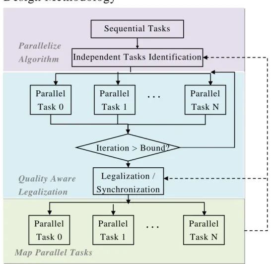
Figure 2: Parallel design methodology which guides the design optimization from algorithm to the parallel platform
For achieving faster runtime, an appropriately co-optimized technique is demanded to handle the communications between the parallelized algorithm and the characteristics of the parallel execution platform. The parallel design methodology, which widely used to algorithms in this thesis, is introduced in this section. In spite of our case study only focuses on 3DIC partitioning on GPGPU, we believe that this design methodology can be applied for other algorithms as well as different parallel architectures.
Fig.2 shows the flow of the parallel design methodology. This parallel design methodology can be divided into three fundamental phases. At first, the parallelize algorithm phase identifies a set of independent parallel tasks from the original
Independent Tasks Identification Sequential Tasks
Legalization / Synchronization
Parallelize Algorithm
Map Parallel Tasks
Parallel Tasks Parallel Task 0 Parallel Task 1 Parallel Task N . . . Parallel Task 0 Parallel Task 1 Parallel Task N . . . Quality Aware Legalization Iteration > Bound?
11
sequential algorithm. This first phase can expose the latent parallelism which could assist with speeding up the runtime of the architecture. Secondly, the quality aware legalization part can relax the synchronization criteria among parallel tasks within a certain execution period. The relaxed synchronization criteria allow the parallel tas ks to search even larger problem space for high quality results. Afterwards, specific mechanisms are added to coordinate concurrent execution of the parallel tasks without violating constraints while considering the quality of the solution. Finally, the last part performs a seamless mapping of parallel tasks to the underlying parallel execution platform. In the last part, taking advantages of the useful features of parallel platform and avoid architectural bottlenecks is the major work. For example, memory conflicts, which are caused by massive communication among parallel tasks, could be the common bottleneck without careful designs. T he dashed lines on the right side of Fig.2 illustrated the circumstances that several iterations usually are required between exposing the parallelism and appropriate optimizations in the parallel platform. Based on this design methodology, the following chapters discuss about how algorithms are designed as well as optimized for GPGPU in detail.
3.3 Design Considerations On GPGPUs
Section 3.3.1 clarifies coalescing of a half warp of threads, and discusses a specified amount of data which are loaded from threads. In Section 3.3.2, the number of threads per block and the number of blocks per grid are determined .
3.3.1 The Amount of Data Used by Threads
In the present CUDA architecture, coalescing global memory accesses is one of the most important performance considerations in programming. Coalescing access is quite useful to possess some local coherence in the texture. When definite access
12
requirements are met, global memory loads and stores by threads of a half warp (or a warp) are coalesced into few transactions by the device [13]. Global memory should be aligned segments of 16- and 32- words to confirm these access requirements: for instance, if every thread all access 32-bits data, then the address which is accessed by the first thread must is a multiple of 64-bytes (16*4 bytes). Fig. 3 explains coalescing of a half warp of threads, such as floats are 32-bit words, and shows global memory as rows of 64-byte aligned segments.
Figure 3: Memory segments and thread in a half warp of thread
In current CUDA devices, an amount of data which is loaded from every thread can be 32-bites, 64- bits or 128-bits. If this amount of data does not meet the requirements, you can use the __align (n) __ instruction to solve problems. However, using 32-bits is the best efficiency. The used data types in our algorithms are integer or float types which all are 32-bit words. Because a GPU normally support 32-bits float type and probably not fully support IEEE 754 specification, some operations may be less accuracy.
3.3.2 The Determined Number of Threads
In CUDA thread hierarchy, threads are grouped into a thread block, and thread blocks are grouped into a grid. The number of threads per block and the number of blocks per grid may affect the performance. How to determine these numbers is depended on algorithms. The number of threads per block multiplied by the number of blocks per grid is the totally number of threads that executes on a GPGPU.
A half warp
64-bytes segment
13
Each multi-processor has 8192 registers in the current CUDA device. If each thread uses 32 registers, a multi-processor only can maintain up to executions of 256 threads simultaneously. If the numbers of present threads more than this figure, it will reduce the efficiency of implementation when a part of data must is accessed in global memory. The maximum threads per blocks of the prevalent CUDA device are 512. For safety, the fixed number of threads per block on proposed programs is 256 when considering the limitation of registers.
Owing to parallel whole particles in N-body simulation, the numbers of blocks per grid is decided the number of particles divide by 256 which presents the number of threads per block. The number of threads that executes on the GPGPU must is larger than the number of particles. Since Nvidia Geforce 9800GT furnishes maximum 65535 grid size, the maximum particles can reach around 16 million which is big enough in N-body simulation. If the number of particles is more than 16 million, the execution of threads may take extremely long latency and cause worst efficiency.
3.4 Optimization Methods On GPGPUs
Although GPGPU provides highly parallel computational capability, without careful designs, the architectural bottleneck can easily limit the potential performance enhancement. Our programs apply two techniques to enhance performance. The first one is coalescing access to alleviate memory bottleneck and the second one is the parallel reduction to speed up the synchronization among all cells. These common optimized topologies are also suitable to other wide-ranging applications.
3.4.1 Coalescing Access
If every multiprocessors have belong global memory caches in the GPU platform , it will need cache coherence protocols and substantially raise the complexity of
14
caches. Since multiprocessors do not do cache in the global memory, the accessed latencies in the global memory are very long. Because of the accessed characteristics of the DRAM, the access in global memory is as continuous as possible.
For continuous access, cells are placed into an array where the addresses are continuous. As shown in Fig.4, we use two arrays to describe this data construction. The array, ptrc, is used to index ptrset array that stores the set of adjacent cells. Each cell is stored as a sequence of the cells that it spans, in consecutive locations in ptrset. When accessing all neighbors within a thread block, this data structure qual ifies the coalescing access. For shorten the memory access latency, all threads in a block coalescing access and use the shared memory as a manual controlled cache.
3.4.2 Reduction Technology
Figure 5: The simple parallel reduction technology Figure 4: Two arra ys that are used to des cribe in Fig. 9-1.
0 1 6 8 12 C P2 P1 D D E B D …… . . ptrc ptrset Cells A B C D E C D E P2 B D
15
Even though we reduce the number of unnecessary sync hronizations, the algorithm still requires some synchronization to collect and calculate information among cells. Therefore we use the parallel reduction technique [14] to speedup these evaluations. As shown in Fig.5, the computation complexity of an array with size of n could be reduced from O(n) to O(log2 n) in the program.
1 2 3 4 5 6 7 8 9 10 11 12 13 14 15 16
__global__ void Devaluate_TSVs(){
__shared__ int sdata[256]; //declare shared memory int tid = threadIdx.x; //threads id in a block int i = blockIdx.x*256+ tid;
sdata[tid] = 0; //initial shared memory //each thread loads one element from global to shared memory
if(i<net_size)sdata[tid] = dnet_highlow[i]; __syncthreads();
if (tid<128) sdata[tid] += sdata[tid + 128]; //do reduction in shared memory __syncthreads();
if (tid < 64) sdata[tid] += sdata[tid + 64]; __syncthreads();
if (tid < 32) warpReduce(sdata, tid); //reduction in a warp //store result for this block to global memory
if (tid == 0) dodata[blockIdx.x] = sdata[0]; }
Table 1: The reduction technique in a warp
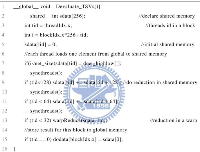
Table 1 illustrates code of the reduction technique in our following programs. This code sums of data by threads. Using __shared__ instruction accesses the shared memory which access speed is quite fast, listed in line 2. In CUDA devices, __syncthreads() instruction, shown in line 8, is a built -in function and denotes that all threads of a block must are synchronized to this point. When the number of needful calculations is less than 32, we have only one warp left. We don’t need to
16
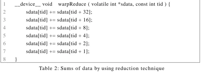
__syncthreads() for less 32 threads per block and saves lot of time. Hence, we construct additional code to handle part in Table 1 line 13. Table 2 demonstrates the reduction technique in a warp.
1 2 3 4 5 6 7 8
__device__ void warpReduce ( volatile int *sdata, const int tid ) { sdata[tid] += sdata[tid + 32]; sdata[tid] += sdata[tid + 16]; sdata[tid] += sdata[tid + 8]; sdata[tid] += sdata[tid + 4]; sdata[tid] += sdata[tid + 2]; sdata[tid] += sdata[tid + 1]; }
Table 2: Sums of data by using reduction technique
3.5 Consideration of Memory Capacity
The total amount of global memory available on the device is almost 1GB in Nvidia Geforce 9800GT. Even though the amount of available memory is big enough for our use in ISPD98 benchmark, the total amount of memory in GPU is still smaller than in CPU. We probe into memory problems when the amount of global memory is not big enough for applications. Because implementations on GPU are only for the N-body simulation of our proposed algorithms, we just discuss the configuration of memory in N-body simulation part.
Finding out independent modules of a hypergraph is the first step . If the memory size of each independent module in a circuit is smaller than the maximum amount of global memory on a GPU, the order and association of the independent module can be easily arranged in the usable memory. These independent modules can practice individually in N-body simulation. Since these modules are self-reliant, there will not have any impact on forces between different independent modules and do not cause
17
influence on solutions. For example in Fig. 6, a given hypergraph is composed by three independent modules: module A, B and C. The total amount of required memory of each module is smaller than 1GB. At first, program performs movements of module A until completely exercising in N-body simulation phase. Then, the program replaces the required second data between CPU and GPU, as well as module B and C are accomplished finally.
What if one of modules is larger than the maximum amount of global memory on a GPU? A casual solution is exchanging information between modules in each time steps. We could see Fig6-3 as an example. First of all, the program partitions the
Module B.C exercise on GPU
A B C
Replace the second data between CPU and
GPU memories Module A exercises on GPU
Figure 6-2: The total amount of memory of each module is smaller than 1GB
A given hypergraph
Independent modules
The maximum amount of memory available on GPU Figure 6-1: Definition and initial hypergraph
A
C B
B C Replace data between
CPU and GPU
A
Module B. C and redundant module A exercises on GPU Mainly Module A
exercises on GPU
Redundant part of A
18
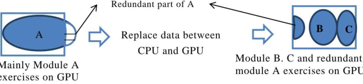
larger module A into main and redundant parts, minimize the size of cutline between these two parts, and copy the duplication between these two parts. Then the program starts to exercise mainly module A in N-body simulation. Since we also copy the duplication, the error between main and redundant parts of module A can be avoided. Next, global memory on a GPU substitutes for next required information, then module B, C and redundant part of module A are fulfilled and operated. Repeat the above steps until simulation terminates. Though the program can frequently substitute information between memories to avoid errors, eternally accessing data cause fiercely latency and lead to worst executed runtime. However, this situation is inevitable under memory limitation. Hence, we also provide second solution which transfers data by blocks instead of time steps and reduce frequently substitutions. The second solution may impact final solutions when main and redundant part of module A still have connections. To avoid likely inaccuracy, the number of connections between these two parts is as few as possible, which could handle by partitioning in the beginning. Consequently, the second solution runs faster than the first solution but gets worst solutions. It depends on the designer’s choice.
3.6 Inter-cell Force Modeling
Electronic circuits usually contain both 2-pin and multi-pin nets. Various models have been proposed to replace multi-pin nets by a group of 2-pin nets. For modeling forces in simulating, our research adopts the traditional model which replaces each net by a clique [15]. For example, for the 4-pin net in Fig.7-1, the clique model is shown in Fig.7-2.
Figure 7-1: Multi-pin nets
19
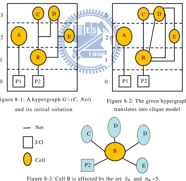
N-body simulation focuses on motions between cells instead situation of nets. To model the forces between cells, the given hypergraph is translated into a speci fic format. Each cell is affected by its own set which is defined as a set of adjacent cells and pins to cell . And is the total number of elements in the set . This following translation model is used for calculating mutual interactions in N -body simulation. For example, Fig.8 illustrates the problem translation into our required format. Fig.8-1 shows a given hypergraph G =(C, Net). Fig.8-2 shows the translation of the hypergraph by using the clique model, and then the interactions between cells are shown. Such as Cell B in Fig.8-3, Cell B is affected by the own set that contains adjacent cells and pins including pin2, cell C, cell D, cell D and cell E.
Figure 8-3: Cell B is affected by the set and =5. I/O Cell Net C D E P2 D B Figure 8-1: A hypergraph G=(C, Net)
and its initial solution
Figure 8-2: The given hypergraph translates into clique model 0 1 2 3 P1 A B P2 C D E 0 1 2 3 A C D E B P1 P2
20
Chapter 4
Case Study: 3D ICs Partitioning
Case Study: 3DICs Partitioning
The partitioning problem formulations and the related works are presented in Chapter 4. The related works are focused on the partitioning algorithms which have been proposed in the past decades. And some symbols used in the following content are also introduced.
4.1 Introduction Of the 3DIC Partitioning
Moore’s Law enables the exponential growth of the chip scale. 3DIC technology enables the vertical integration of a large scale system onto the multiple layers of the same die or the same package [16]. The multilayer structure of the 3DIC technology makes it even more computational expensive for EDA tools to achieve optimization goals. The future EDA tools are required to handle the sheer amount of system complexity which requires enormous computation power to sustain the satisfactory performance. Parallel computing has been considered as a solution to meet the soaring requirement [ 17 ]. Multi-core architectures, such as general purpose graphic processing unit (GPGPU), have become the mainstream of the future computing systems. Through expanding parallelism in applications, GPGPU can exploit parallelism and achieve superior performance.
Partitioning is in the first step of physical design optimization flow [18]. For a 3DIC, partitioning divides cells into K sub-groups and assigns these groups to different layers. The signals between layers are connected by the Through Silicon
21
Vias (TSVs) which generally occupy larger chip area t han conventional vias. Thus the optimization result of 3DIC partitioning determines the total number of TSVs between layers and has significant impact on several imperative design issues such as number of TSVs, footprint area constraint, timing, thermal distribution, as well as the fabrication yield. To reduce the cost, the goal in this study case is to minimize the number of TSVs under the footprint constraints.
This thesis proposes FDPrior, a highly parallel 3DIC partitioning algorithm based on force-directed scheme with prioritized layering mechanism. FDPrior is among the first to adopt a non-heuristic technique by using force-directed [ 19] methods to approach 3DIC partitioning problems. These force-directed methods extend the conventional concepts of direct N-body simulation. Chapter 5 will introduce the flow of FDPrior in detail.
4.2 Related Work: Partitioning Algorithms
Partitioning has been extensively researched during the past decades. To resolve partitioning problems, various approaches have been proposed . We have surveyed the following four related works.
The first group of algorithms adopted heuristic approaches to enable eas y implementation and return acceptable solution quality. The representative example of this group is the FM algorithm. FM was first proposed by Fiduccia and Mattheyses, and is widely used in solving various partitioning problems. FM used a greedy -like approach to move the cell which could return the maximum gain. However, the runtime of FM gets significantly worse with the increasing number of cells. Besides, the algorithm itself is prone to fall into a local optimum and returned a sub -optimal result.
22
The second group used deterministic approaches, such as ILP (Integer Linear Programming), to find out the optimal solution. Jiang et.al [20] used the ILP approach to formulate the 3DIC partitioning problem and was able to find the minimum number of TSVs with constrained footprint. The downside of this approach was the extremely long run time which was impractical for a system with a large number of cells.
The third group used multilevel approach to solve the partitioning pro blem hierarchically. hMetis [21] is one of the most widely used algorithm in this group. hMetis started by repeatedly combining cells into groups of cells ( this process called coarsening). When the numbers of cells got smaller and reached an acceptable level, hMetis performed FM partitioning followed by un-coarsening the cell groups to a finer-grain level. The process was repeated until all the created cell groups were un-grouped to the finest level.
With the soaring system complexity in the future 3DIC design, parallel processing on many-core architecture is considered as a solution to enable the scalable computing capability for future EDA tools. PP3D was proposed speed up the 3DIC partitioning by adopting parallel processing scheme. PP3D extended the fundamental ideas of FM algorithm, and adde d the ability to identify the independent cells which could be moved simultaneously. Compared with the original FM, PP3D achieved one order of runtime speedup while returning the similar solution quality.
4.3 3DIC Partitioning Problem Formulation
This subsequent section will introduce how the 3DIC partitioning problem is modeled for FDPrior algorithm. The definitions of the partitioning problem and variables are described here.
23
4.3.1 The Structure of 3DICs
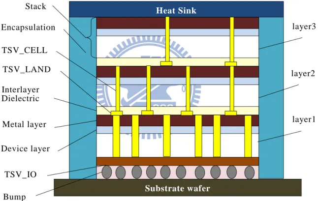
Fig.9. shows a simple example of the structure of a 3DIC [22]. All the layers are stacked up vertically. A TSV_IO connects the layer_1 to the bump of a package pin. A TSV, which consists of a TSV_CELL and a TSV_LAND, connects signals between two internal adjacent layers. A TSV_CELL connects to the upper metal l ayer and a TSV_LAND is a landing pad placed on the lower metal layer. In the partitioning, each TSV is modeled as a cutline between the neighboring layers. The total number of TSVs in this thesis contains both the TSV_IOs and TSVs.
4.3.2 Variable Definitions
1. A circuit is modeled by a hypergraph G=(C, Net) where with a set of nets Net that connect to two or more cells and a set of cells C that each cell C. And
is the given area of cell .
TSV_CELL TSV_LAND layer3 layer2 layer1 Stack ed die Encapsulation TSV_IO Device layer Metal layer Bump Interlayer Dielectric Heat Sink Substrate wafer
24
2. is the total area of all cells in layer_j and is the total area of the TSV_IO cells. is the average layer area of a 3DIC. The area constraint of each layer is defined as follows:
(3)
) (4)
(5)
The maximum and minimum bounds of layers are set as and respectively. is a given constant that decides the range of area bounds. The
overflow area is that multiplies the ratio of . And the minimum and maximum area bounds are the average layer area of a 3DIC subtracted or added this overflow area.
3. Equation 6 defines the displacement of the cell .Where represents the current position of , represents the position of from the previous optimization iteration, and the displacement of between two iterations.
(6)
, and are all in the z-direction. The sign of guides the direction of cell .
4. During the optimization, each cell can be in either the fixed state or mobile state. A cell in the mobile state can move freely in response to the inter -cell forces while a fixed cell stays at the current position.
4.3.3 Problem Description
The 3DIC partitioning problem can be formulated as a hypergraph multilayer partitioning problem. Given the hypergraph of a netlist and area constraint (
), a partitioning algorithm divides the set of cells C into K layers
25
Chapter 5
FDPrior Algorithm
FDPrior Algorithm
Chapter 5 introduces our proposed algorithm, FDPrior [ 23 ]. The main contributions of FDPrior could be categorized into three folds: 1) massive algorithmic parallelism exploited by multi-core GPGPU computing systems 2) a force -directed approach to achieve high result quality 3) bottom -up prioritized layer construction to minimize synchronization overhead.
FDPrior enables a massive computation parallelism by N-Body simulation method which simulates motions of all cells independently. N -Body simulation phase adopts a non-heuristic approach of force-directed method to simulate forces among cells. However, N-body simulation needs fierce mathematical computations for interaction of N particles among a dynamic system. Such N-body problems encounter a formidable challenge to the numerical analysis and computer hardware. Hence, the applications of N-body simulation are particularly suitable for modern multi-core platforms. In partitioning problem, conventional approaches usually define the layer space at first and then optimize solutions on pre-defined layer spaces. However, in parallel algorithm, this method would result in much synchronization which is used to obtain information among cells, such as the distribution. In third fold, FDPrior does not define the layer spaces in the beginning. Instead, the layer space is gradually stacked up by the bottom-up layer construction. This innovative method can significantly reduce the number of synchronizations and gain faster runtime.
In addition to returning better results, FDPrior is designed to take advantage of the scalable computing capability enabled by multi -core computing systems. When
26
compared with PP3D [24] and the conventional FM [25] algorithms, FDPrior can achieve up to 3.35X and 303.66X times faster runtime on ISPD98 benchmark. Not only finishing the execution faster, FDPrior also returns better results which are in average 7.71X and 5.95X better in terms of total TSV numbers.
5.1 FDPrior algorithm
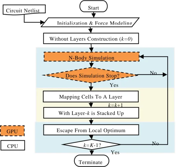
The algorithm flow is illustrated in Fig.10. The orange parts implement on the GPU platform, as well as the white parts execute on CPU. The algorithm is composed of three phases, including N-body simulation, mapping cells to a layer, and escape
Figure 10: The flow chart of FDPrior algorithm.
Independent module Circuit Netlist
Escape From Local Optimum Mapping Cells To A Layer Initialization & Force Modeling
N-Body Simulation
Does Simulation Stop?
Terminate k=K-1?
Start
CPU GPU
Without Layers Construction (k=0)
With Layer-k is Stacked Up k=k+1
Yes
No Yes
27
from local optimum. N-Body simulation phase simulates the movement of each mobile cell based on the forces impacted on it. The second phase picks appropriate cells and maps them to a layer. The first two phases limit the optimization search within a regional area and could fall into a local optimum. Thus the third phase enables a mechanism to escape from local optimum through disturbing the unfixed cells. The above phases will be repeated K-1 times to determine the lower K-1 layers. The remaining mobile cells after K-1 iterations are directly placed into the layer_ K. Details of each phase are discussed in the below sections.
5.1.1 Phase1: N-body Simulation
FDPrior employs the non-heuristic approach to calculate the forces. N-body simulation numerically approximates the motion of each cell in a system. Each cell in a netlist is modeled as a body and be moved independently. Consequently, there has massive parallelism and exploits by the GPGPU platforms. We separate the force into two fundamental components. First, the hold force will give each cell a tendency to stay in the current position. The second component is an attractive force, which is induced by the inter-cell forces to move cells to towards the equilibrium position. These two forces pull each other until the total force is zero; and the system reaches a static equilibrium.
5.1.1.A Hooke’s Law
Many problems seem new but actually not. The quadratic placement techniques had been used for the placement problem in a long time. We can refer the previous methods on placement and make modifications for solving partitioning in 3DICs. Accordingly, FDPrior adopts old solutions of the placement problems and assumes the Hooke’s law to describe the motions of force. In quadratic placement problem, many
28
algorithms use the springs or extra forces by Hooke’s law to obtain better solutions, e.g. Quinn published in 1975 [26]. This method is usually celled force-directed approach in the EDA field.
Simulating mobile cells in a free space may appear vibration when applying gravitational forces that describes in Section 2.2. In our experience, the vibration could take a long time to reach a stable state by using Equation 1 as the force equations. We practice the general rectilinear motion formulae to describe the motion along a straight line. Since there are not frictions in simulation, the accumulated speed keeps each body moving even after they have arrived the meeting point, and results in a two-body vibration situation. According to practical implementations, f the vibration mode can rarely provide improvement on the solutions. In the simulation, the vibration mode happens when the direction of a body’s acceleration is opposite to its velocity. For this reason, spending too much time on the simulation of the vibration mode is unnecessary and considered redundant.
In physics, Hooke's law of elasticity is an approximation that expresses the extension of a spring with the load applied to it. Hooke's law simply presents that strain is directly proportional to stress. The common application of Hooke’s law is spring application. To avoid vibration and obtain quick convergence, FDPrior adopts the forces exerted by the springs, which are defined by Hooke’s law. Hooke’s law states mathematically in Equation7 where F is the restoring force exerted by the spring.
(7)
Where x is the displacement of this spring's end from its equilibrium position; and k is the spring constant. A negative sign on the right hand side of Equation 7 shows always opposite direction between displacement and restoring force. FDPrior perform force-directed method to solve equations of forces instead by linear solver.
29
5.1.1.B Hold Force
The hold force is defined in Equation 8. , defined by the area of cell , is the spring constant which affects the strength of the hold force.
(8)
The negative sign presents this cell want to stay in the current position. When the area of a cell is large, this cell has larger momentum a nd is more difficult to be moved.
5.1.1.C Attractive Force
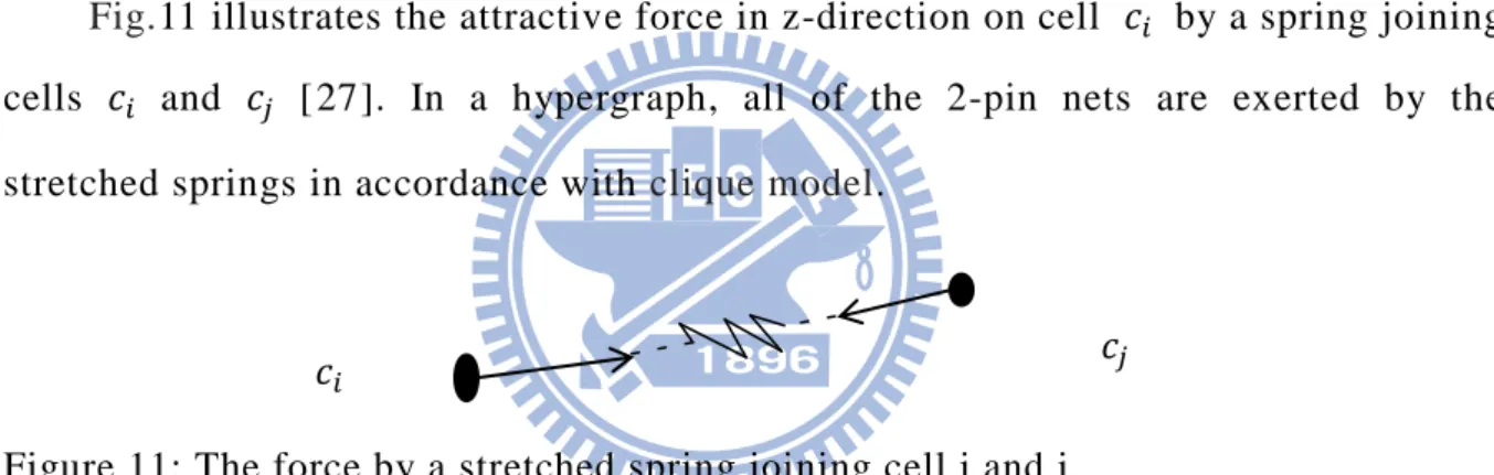
Fig.11 illustrates the attractive force in z-direction on cell by a spring joining cells and [ 27]. In a hypergraph, all of the 2-pin nets are exerted by the stretched springs in accordance with clique model.
Figure 11: The force by a stretched spring joining cell i and j.
The attraction force between two bodies forms a tendency to pull the bodies closer to each other at every simulation step. The attractive force between cells is defined in Equation 9. The final attractive force is the accumulated forces impacted on a cell . (9)
In Chapter 3, we mentioned that FDPrior adhere the clique model to modify the given hypergraph, which is translated from the multi-pin nets to a group of 2-pin nets by clique model. All the weight of each 2-pin net is same and set to unit in a system. The formulation of the force in the clique by Hooke’s law is equivalent to Equation 8.
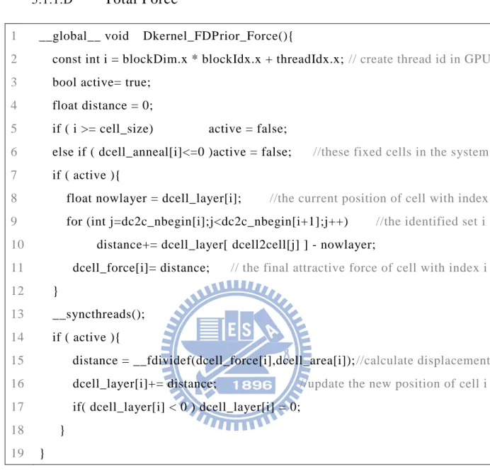
30 5.1.1.D
Total Force
1 2 3 4 5 6 7 8 9 10 11 12 13 14 15 16 17 18 19__global__ void Dkernel_FDPrior_Force(){
const int i = blockDim.x * blockIdx.x + threadIdx.x; // create thread id in GPU
bool active= true; float distance = 0;
if ( i >= cell_size) active = false;
else if ( dcell_anneal[i]<=0 )active = false; //these fixed cells in the system
if ( active ){
float nowlayer = dcell_layer[i]; //the current position of cell with index
for (int j=dc2c_nbegin[i];j<dc2c_nbegin[i+1];j++) //the identified set i
distance+= dcell_layer[ dcell2cell[j] ] - nowlayer;
dcell_force[i]= distance; // the final attractive force of cell with index i
}
__syncthreads(); if ( active ){
distance = __fdividef(dcell_force[i],dcell_area[i]);//calculate displacement
dcell_layer[i]+= distance; //update the new position of cell i
if( dcell_layer[i] < 0 ) dcell_layer[i] = 0; }
}
Table 3: The code of the calculated forces in the N-body simulation phase
The total force is the sum of the hold force and attractive force. The new cell positions are efficiently computed by solving Equation 10 for .
(10)
The N-Body Simulation phase terminates when the number of iterations reaches the threshold level or the total number of iterations exceeds a configured limit. In each layer space, configured limit is 2000 in our experimentation. The threshold level is defined as * distribution ratio where is an empirical number. The range used in
31
this algorithm is = 0.95. And the distribution ratio is the total number of mobile
cells which fall in the constructed layers divided by the rest of the mobile cells. In other words, * distribution ratio means that the majority of cells exercise enough
and already drop to the lower layer by the connected nets.
Table 3 shows the calculations of forces in the N-body simulation phase. Line 6 percolates already fixed cells in a system. Line 7-12 calculates each attractive force with cell by creating a thread with index i. Because throughput of single-precision floating-point division takes some cycle, we use __fdividef functio n to accelerate for division, shown in line 15. This __fdividef(x,y) function means x divided by y and provides a faster math version. Both the regular floating -point division and __fdividef(x,y) have the same accuracy. But __fdividef(x,y) delivers a result of zero and cause inaccuracy when 2126 < y < 2128. Fortunately, the areas of every cells in the ISPD98 benchmark are not bigger than 2126. Line 14-18 arranges the data and updates the new positions of cells. Since the I/O pins are located in the bottom layer, the positions cannot be lower than 0. In case this situation occurs, we add a refinement in line 17.
5.1.2 Phase 2: Mapping Cells To A Layer
In the Mapping Cells To A Layer phase, the layer space is constructed by gradually stacking up cells from the bottom of a layer. Since it is a bottom -up approach, cells at lower positions have higher priorities to be included in this layer. When more cells are included in this layer, the area of this layer will increase. And FDPrior will search the best layer boundary (with minimal cutline) between the minimum layer area bound ( ) and maximum layer area bound ( ) which were defined in Chapter 3. These cells which are mapped into this layer will be changed into the fixed state, while others remain in mobile states.
32
In other words, FDPrior will gradually search cells which are located in lower positions and straightly put them in this layer until the area of this layer reaches the minimum layer area bound. For example, these cells with index 1 … p are successively mapped into a layer. Then FDPrior estimates the cutline and save data in the buffer when each cell moves until the area of this layer reaches the maximum layer area bound. Suppose these cells with index p+1 … q are already handled and each cell has its own cutline. Finally, the program will seek out the minimum cutline between cells with index from p+1 to q, as well as set the appropriate cells into fixed states. If the cell with index g has the minimal cutline, cells with index g+1 … q will set to freedom in a system. In conclusion, only these cells with index 1 … p, p+1 … g are firmly mapped into these layer and turned states into the fixed states.
In the program beginning, there does not define any layer spaces. And all the cells of the given hypergraph are in the mobile states. Each layer space will b e stacked up after repeating executes the Mapping Cells To A Layer phase. Until the lower K-1 layers all are successively implemented, the remaining mobile cells in the system will be directly placed into the layer_K.
5.1.3 Phase 3: Escape From Local Optimum
The previous two phases limit the optimization search within a regional area and the solution may fall into a local optimum. FDPrior adds an approach to escape from the possible local optimum by disturbing certain m obile cells based on Equation 10.
/
/ ) (11)
33
5.2 Experimental Results
The target GPGPU platform of FDPrior is Nvidia Geforce 9800GT [28]. All the experiments are conducted on a 2.66GHz Intel® Core(TM) i7 -920 CPU sprinting CentOS 5.5 with 6GB of memory. This research adopts the ISPD98 benchmark suite to evaluate the algorithms [29]. ISPD98 contains a wide range of varieties, which is listed in Table 4. The indicates the unbalance of layers and the area footprint constraint. The number of desired layers and are different when considering characteristics in every case are distinct. If the chip area is immense, we donate this chip more freedom in the area bounds, such as the chip area in ibm18 is larger then the given constant will be slightly great. The numbers of threads per block are 256 in all cases when considering the limitation of registers. Consequently, the total number of threads that we implemented in the GPGPU platform is 256* the number of blocks per grid.
Bench #Block #cells #nets #I/Os #layers
ibm01 56 12506 14111 246 4 10 ibm02 78 19342 19584 259 4 10 ibm03 108 22853 27401 283 4 10 ibm04 126 27220 31970 287 4 10 ibm05 112 28146 28446 1201 4 10 ibm06 137 32332 34826 166 4 10 ibm07 189 45639 48117 287 5 12 ibm08 200 51023 50513 286 5 12 ibm09 239 53110 60902 285 5 12 ibm10 295 68685 75196 744 5 12 ibm11 319 70152 81454 406 5 12 ibm12 303 70439 77240 637 5 12 ibm13 390 83709 99666 490 6 15 ibm14 598 147088 152772 517 6 15 ibm15 730 161187 186608 383 6 15 ibm16 743 182980 190048 504 6 15 ibm17 742 184752 189581 743 6 15 ibm18 823 210341 201920 272 6 15
34
Fig.12 compares the average number of TSVs generated by FDPrior, PP3D [22] and MLFM algorithms. PP3D leverages the fundamental ideas of FM algorithm, and adds the ability to identify the independent cells. MLFM represents the exten ded conventional FM algorithm which considers multilayer partitioning. FDPrior obtains much better qualities than PP3D and MLFM in every benchmark. The experimental numbers are the average of 30 runs. The average numbers of TSVs which execute on the algorithms in ISPD98 benchmark are listed in Table 5.
Figure 12: Comparison of average solutions on the algorithms.
When comparing with PP3D and MLFM, FDPrior demonstrates an average of 7.71X and 5.95X better solution quality respectively. Since PP3D introduces the primary ideas of FM algorithm, the solutions of PP3D is a bit of near to the solutions of MLFM. FDPrior accomplishes an absolutely different algorithm by using N-body algorithm and creates coarser grain than others. That is the reason that FDPrior can perform better solution qualities.
From the distribution of 30 runs, FDPrior is more stable on solution qualities than PP3D and MLFM algorithms. Fig.13 shows the solution qualities of PP3D are distributed across a wider range than FDPrior in ibm04. FDPrior also achieves 3.35X
1 .E+0 3 1 .E+0 4 1 .E+0 5 1 .E+0 6 #T SV s FDPrior PP3D MLFM IBM1 8 IBM1 7 IBM1 6 IBM1 5 IBM1 4 IBM1 3 IBM1 2 IBM1 1 IBM1 0 IBM0 9 IBM0 8 IBM0 7 IBM0 6 IBM0 5 IBM0 4 IBM0 3 IBM0 2 IBM0 1