WiMAX 迴旋渦輪碼技術與 數位訊號處理器實現

國 立 交 通 大 學

電子工程學系 電子研究所碩士班

碩

士

論

文

WiMAX 迴旋渦輪碼技術與

數位訊號處理器實現

WiMAX Convolutional Turbo Code Technology

and Digital Signal Processor Implementation

研 究 生：曾劭學

指導教授：林大衛 博士

WiMAX 迴旋渦輪碼技術與

數位訊號處理器實現

WiMAX Convolutional Turbo Code Technology

and Digital Signal Processor Implementation

研究生:曾劭學 Student: Shao-Hsueh Tseng

指導教授:林大衛 博士 Advisor: Dr. David W. Lin

國立交通大學

電子工程學系 電子研究所碩士班

碩士論文

A Thesis

Submitted to Department of Electronics Engineering & Institute of Electronics College of Electrical and Computer Engineering

National Chiao Tung University in Partial Fulfillment of the Requirements

for the Degree of Master in

Electronics Engineering October 2009

Hsinchu, Taiwan, Republic of China

WiMAX 迴旋渦輪技術

與數位訊號處理器實現

研究生:曾劭學 指導教授:林大衛 博士

國立交通大學

電子工程學系 電子研究所碩士班

摘要

IEEE 802.16e 無線通訊標準中，於系統的傳送端訂定了前向誤差

更正編碼的機制，藉此降低通訊頻道中雜訊失真的影響。通道編碼為

本論文的重點。

本篇論文在於研究 IEEE 802.16e OFDMA 所訂定的迴旋渦輪

碼（CTC）系統並實現在數位訊號處理器(DSP)。闡明迴旋渦輪碼的

雙二位元循環遞迴系統迴旋（duo-binary CRSC）編碼以及利用最大

對數事後機率(max-log-MAP)進行 BCJR (Bahl `Cock `Jelinek 和

Raviv 四位研究者做為命名)解碼演算法。我們利用 C 語言驗證系統

演算法上的正確性，以及補償 max-log-MAP 導致的效能損失，並在

接著在 TI C6416 DSP 平台，我們改變格子圖順序，以及利用 DSP

內建函式達到平行運算，並且有效改善解碼器的運算速度。原始解碼

器的部分僅可達到約每秒 800K 位元的處理速度，改善後解碼器的速

度增進約 2 倍，進而可以達到每秒 1500K 位元的處理速度。

WiMAX Convolutional Turbo Code Technology

and Digital Signal Processor Implementation

Student: Shao-Hsueh Tseng Advisor: Dr. David W. Lin

Department of Electronics Engineering

& Institute of Electronics

National Chiao Tung University

Abstract

In the IEEE 802.16e wireless communication standard, a forward error

correction (FEC) mechanism is presented are the transmitter side to

reduce the noisy channel effect. The focus is on the channel coding.

The focus of this thesis is the research of the convolutional turbo code

(CTC) defined in IEEE 802.16e OFDMA and implement on the C6416

DSP. We explain the duo-binary circular recursive systematic

convolutional encoding (duo-binary CRSC) and use BCJR decoding

algorithm by max-log-MAP. We employ the C program to insure the

correctness of our algorithm and compensate the performance loss by

max-log-MAP, furthermore, simulate the CTC for different modulations

in AWGN.

Then, we implement on TI C6416 DSP, changing trellis order and

using intrinsic function to achieve parallel operation. Therefore, we

improve decoder operation speed efficiently. For original decoder just can

achieved a processing rate of 800 Kbps . For improved decoder , which is

誌謝

本篇論文的完成，首先要特別感謝我的指導教授林大衛博士，在我進入交大 電子所開始，不論是課業或是研究上的困難，老師總能細心的給予適時方向去解 決問題，使我學到了分析以及解決問題的能力。此外老師對於學生的認真以及親 切樂觀的態度更是深遠影響了我，使我在研究所的這幾年得到了學術以外更重要 的智慧。 此外，由衷的感謝通訊電子與訊號處理實驗室所有的成員，包含各位師長、 同學、學長姐以及學弟妹們。特別感謝吳俊榮學長、林鴻志學長、王海薇學姐和 盧世榮學弟對我在學術上的不吝指導與建議，謝謝你們幫我解決了許多通訊方面 的疑問。感謝 95 級佳楓學長的指導，96 級凱暐、志偉、豐進、清德、辰彥等實 驗室成員，以及陳紹基老師的學生嘉洵跟靖順，平日和我一起念書、討論、玩耍， 讓我的研究生涯擁有美好的回憶。期待各位夥伴們畢業後都有不錯的發展。 最後，必須感謝我的家人，我父母親給予我的支持，使我在外地讀書時能無 後顧之憂，感謝他們的支持，也謝謝所有幫助過我、陪我走過這段歲月的人 曾劭學 民國 98 年 11 月 於新竹

Contents

1 Introduction 1

1.1 Scope of the Work . . . 1

1.2 Organization of this Thesis . . . 2

2 Overview of CTC in IEEE 802.16e OFDMA 3 2.1 Convolution Turbo Code Specification [1] . . . 3

2.1.1 Randomizer [1] . . . 4

2.1.2 CTC Encoder In IEEE 802.16e OFDMA [1] . . . 6

2.1.3 1/3 CTC Encoder [1] . . . 8

2.1.4 CTC Interleaver [1] . . . 10

2.1.5 CTC Tail-Biting [1], [4] . . . 11

2.1.6 Subpacket Generation (Channel Interleaver or Interleaver and Punc-turing) [1] . . . 14

2.1.7 Modulation [1] . . . 19

2.1.8 Demodulation for Bit-Interleaved Coded Modulation [3] . . . 19

2.2.1 The Turbo Decoding Algorithm [5] . . . 23

2.2.2 Decoding Rule for CRSC Codes with Non-binary Trellis [8] . . . 25

2.2.3 Simplified Max-Log-MAP Algorithm for Double-Binary CTC [8] . . . 28

3 DSP Implementation Environment 33 3.1 The DSP Board [12] . . . 33

3.2 The DSP Chip [12] . . . 34

3.2.1 Central Processing Unit [12] . . . 36

3.2.2 Memory [14] . . . 39

3.3 TI’s Code Development Environment [15] . . . 40

3.4 Code Development Flow [17] . . . 42

3.5 Code Optimization on TI DSP Platform . . . 42

3.5.1 Compiler Optimization Options [17] . . . 44

3.5.2 Software Pipelining [18] . . . 46

3.5.3 Macros and Intrinsic Functions [17] . . . 47

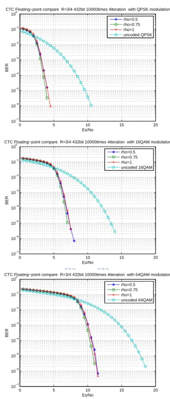
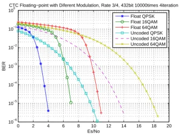
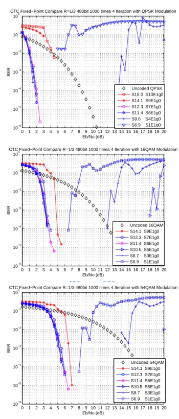
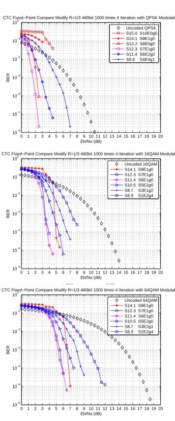
4 Fixed-Point Implementation of CTC Encoder and Decoder 48 4.1 Performance in AWGN Channel with Floating-Point Processing . . . 48

4.2 Performance in AWGN Channel with Fixed-Point Processing . . . 49

4.2.1 Scaling Method [22] . . . 53

4.2.2 Clipping Method [19], [20] . . . 60 5 Speeding Up of DSP Implementation 67

5.1 Speed of DSP [17] . . . 67

5.2 Original State Order [22] . . . 71

5.3 Arrange State Order to Achieve Parallelism . . . 73

5.4 Comparison of Speed . . . 78

5.4.1 Comparison of Original and Improved Codes in Additions, Multiplica-tions and Intrinsic FuncMultiplica-tions . . . 78

5.4.2 Processing Rate of CTC Decoder . . . 86

6 Conclusion and Future Work 89 6.1 Conclusion . . . 89

6.2 Future Work . . . 90

List of Figures

2.1 Use of CTC in transmitter and receiver of IEEE 802.16e OFDMA (from [1]). 4

2.2 PRBS for data randomization (from [1], Fig. 337). . . 6

2.3 Structure of CTC in transmitter ans decoding in receiver (based on [1]). . . . 7

2.4 CTC encoder (base on [1]). . . 9

2.5 CTC rate 1/3 encoder flow chart [22]. . . 9

2.6 CTC encoding slot concatenation for different rates [1]. . . 11

2.7 CTC channel coding per modulation (modified from [1]). . . 12

2.8 CTC interleaver in two steps (modified from [1]). . . 13

2.9 Block diagram of CTC channel interleaving scheme (from [1]). . . 17

2.10 QPSK, 16-QAM, and 64-QAM constellations (from [1]). . . 20

2.11 Metric partitions of the 16-QAM constellation (from [3]). . . 23

2.12 Block diagram of a turbo decoder (from [5]). . . 24

2.13 CTC trellis structure of duo-binary convolutional code with feedback encoder (from [8]). . . 26

3.1 Sundance’s SMT395 module (from [11]). . . 34

3.3 C64x cache memory architecture [14]. . . 40 3.4 Code development flow for C6000 [17]. . . 43 3.5 Software-pipelined loop [17]. . . 46 4.1 Performance of CTC at different ρ values under three modulations with 288

information bits. . . 50 4.2 Performance of CTC at different ρ values under three different modulations

with 432 information bits. . . 51 4.3 Performance of CTC at 288-bit and ρ = 0.75 with different modulations

em-ploying floating-point computation at 4 iterations. . . 52 4.4 Performance of CTC at 432-bit and ρ = 0.75 with different modulations

em-ploying floating-point computation at 4 iterations. . . 52 4.5 Hypothetical reference CTC decoder implementation with marking of

fixed-point data format at various place. . . 53 4.6 CTC fixed-point truncation parameters (modified from [22]). . . 54 4.7 Illustration of fixed-point data formats with the scaling method, where Q11.4

may be replaced by other setting (such as Q9.6 or Q14.1) depending on code rate and operating condition. . . 55 4.8 CTC decoding at different bit numbers with different modulations. . . 56 4.9 Performance with scaling of various quantities in CTC decoding to avoid

over-flow at high SNR. . . 57 4.10 Performance of CTC with different scale factors under three modulations with

4.11 Performance of CTC with different scale factors under three modulations with

432 information bits. . . 59

4.12 Fixed-point data format with the clipping method. . . 61

4.13 Performance of CTC at different clipping ranges under three modulations with 288 information bits. . . 63

4.14 Performance of CTC at different clipping ranges under three modulations with 432 information bits. . . 64

4.15 Performance of rate 1/2 CTC with 288 information bits with floating-point decoding vs. fixed-point under clipping method. . . 65

4.16 Performance of rate 3/4 CTC with 432 information bits with floating-point decoding vs. fixed-point under clipping method. . . 66

5.1 Graphical representation of the amem4() and the max2() intrinsics [17]. . . 69

5.2 Graphical representation of the dotp2() intrinsic [17]. . . . 69

5.3 Graphical representation of packXX2() intrinsics[17]. . . . 70

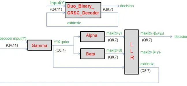
5.4 Overall encoder and decoder architecture. . . 71

5.5 Trellis diagram, every branch in the trellis connecting at time k − 1 to a state at time k. . . . 74

5.6 Arrangement of trellis order for forward and backward metrics. . . 75

5.7 Use of the packXX2() intrinsics for forward metric . . . . 75

5.8 Improved C code for the alpha() function. . . 78

5.9 Assembly code of the alpha() function (1/5). . . 79

5.11 Assembly code of the alpha() function (3/5). . . 81

5.12 Assembly code of the alpha() function (4/5). . . 82

5.13 Assembly code of the alpha() function (5/5). . . 83

List of Tables

2.1 CTC Channel Coding Schemes for Each Modulation Method . . . 5

2.2 Circulation State Look-Up Table (SC1 and SC2) [1, Table 573] . . . 14

2.3 Parameters for the Subblock Interleavers . . . 16

2.4 Bit Metric for Method-ML and Method-LLR . . . 22

2.5 Amount of Additions, Multiplications and Max Operations for Soft-Output Decoding of One Component Code Once, Where Number of Information Bits = 480 . . . 32

3.1 Functional Units and Operations Performed [12] . . . 37

4.1 Coding Gain Performance of Rate-1/2 CTC in AWGN at BER = 10−5 _with Floating-Point and Fixed-Point with Scaling Method Computation . . . 60

4.2 Coding Gain Performance of Rate-3/4 CTC in AWGN at BER = 10−5 _with Floating-Point and Fixed-Point with Scaling Method Computation . . . 60

4.3 Coding Gain at Rate 1/2 with 288 Information Bits CTC in AWGN at BER = 10−4 _{with Floating-Point Computation and Fixed-Point Computations with} Scaling Method and Clipping Method . . . 62

4.4 Coding Gain at Rate 3/4 with 432 Information Bits CTC in AWGN at BER = 10−4 _{with Floating-Point Computation and Fixed-Point Computations with}

Scaling Method and Clipping Method Computation . . . 62

5.1 TMS320C64X Compiler Intrinsics [17]. . . 68

5.2 Overall Encoder and Decoder Block Cycles . . . 72

5.3 Speed Up in Channel Interleaver . . . 72

5.4 Profile of Duo Binnary CRSC decoder with QPSK Modulation for 480 In-formation Bits, Rate 1/2 Coding in One Iteration . . . 73

5.5 Profile of Improve Duo Binnary CRSC Decoder with QPSK Modulation for 480 Information Bits, Rate 1/2 Coding in One Iteration . . . 77

5.6 Speed Up in Decoding of One Data Block with QPSK Modulation for One Iteration . . . 77

5.7 Numbers of Intrinsic calls and arithmetic operations in Original Code for CTC Decdoding . . . 85

5.8 Numbers of Intrinsic Calls and Arithmetic Operation in Improved Code . . . 86

5.9 Information Data Processing Rate Calculated from CCS for Original Code for 480 Information Bits, Rate 1/2 Coding . . . 87

5.10 Information Data Processing Rate Calculated from CCS for Improved Code for 480 Information Bits, Rate 1/2 Coding . . . 87

5.11 Comparison of Decoder Speeds for Tail-Biting CC, CTC, and LDPC Calcu-lated from CCS . . . 88

Chapter 1

Introduction

1.1

Scope of the Work

Digital wireless transmission is a trend in the next generation of consumer electronics. Due to this demand high data transmission rate and mobility are needed. The OFDM modulation technique for wireless communication has been a main stream in recent years. IEEE has completed several standards, including the IEEE 802.11 series for LANs (local area networks) and IEEE 802.16 series for MANs (metropolitan area networks), based on OFDM technique. Our study is based on the IEEE 802.16 standard [1] which specifies the air interface of mobile broadband wireless multiple access systems providing multiple access. In wireless communication, the transmitted signals are easily interfered and distorted by variance things sources such as the crowd traffic, bad weather, the obstacle of buildings, etc. Digital wireless transmission with multimedia contents such as audio and video is a trend. These services often exhibit high data rates and require high quality reproduction. To improve the robustness of the wireless communication against the noisy channel condition, the FEC (forward-error-correcting coding) mechanism is a must in almost every commercial communication standard, including the IEEE 802.16.

Mobile WiMAX. In addition, the puncture and M-ary modulation are used after encoder. A number of studies have been conducted using BCJR algorithm [6] as the turbo decoding. There have been numerous studies in the literature dealing with different decoding algo-rithm. However we need to reduce the complexity for actual digital signal processor (DSP) implementation. For convolutional turbo codes, we arrange trellis order to achieved parallel operation.

In this thesis, we focuss on the study of the simulation and the DSP implementation of the CTC in the IEEE 802.16 standard, We first study the encoding and decoding techniques. Then we perform computer simulation to investigate the coding performance. Finally, we optimize CTC on the DSP with fixed-point computation.

1.2

Organization of this Thesis

This thesis is organized as follows.

• Chapter 2 introduces the CTC (convolutional turbo codes) of IEEE 802.16e

specifica-tions.

• Chapter 3 describes the DSP implementation environment.

• Chapter 4 discusses simulation and DSP implementation of the CTC. • Chapter 5 discusses the optimization of CTC decoder on DSP.

Chapter 2

Overview of CTC in IEEE 802.16e

OFDMA

The convolutional turbo code (CTC) is one mandatory channel coding scheme in Mobile WIMAX. In this chapter, We introduce the encoding and the decoding methods for the CTC in IEEE 802.16e OFDMA.

2.1

Convolution Turbo Code Specification [1]

The mandatory channel coding scheme used in IEEE 802.16e OFDMA is as shown in Fig. 2.1. The input data stream is processed by the randomizer to clean up the bit correlation, and then each data block is encoded by the convolutional turbo encoder. The block-by-block coding makes the convolutional turbo code effectively a block code. However, we do not implement the repetition block, which can be used to further increase the signal-to-noise-ratio (SNR) margin over the modulation and FEC mechanisms, for the channel coding procedures in IEEE 802.16e. Repetition block can be applied only to QPSK modulation. Reader interested in the repetition block can refer to relevant material in [1].

To make the system more flexibly adaptable to the channel condition, 32 coding-modulation schemes are defined in IEEE 802.16e, as shown in Table 2.1. The different coding rates are

Figure 2.1: Use of CTC in transmitter and receiver of IEEE 802.16e OFDMA (from [1]). made by puncturing of the native convolutional turbo code. The puncturing mechanism in convolutional turbo coding can provide variable code rates through one convolutional turbo encoder.

2.1.1

Randomizer [1]

The randomizer is a pseudo random binary sequence (PRBS) generator defined by the polynomial 1 + X14_{+ X}15_{, as depicted in Fig. 2.2. Data randomization is performed on all}

data transmitted on the downlink (DL) and uplink (UL), except the frame control header (FCH). The randomization is initialized on each FEC block.

If the amount of data to transmit does not fit exactly the amount of data allocated, padding of 0xFF (“1” only) shall be added to the end of the transmission block, up to the amount of data allocated. Here, the amount of data allocated means the amount of data that corresponds to the amount of slots bNs/Rc, where Ns is the number of the slots allocated for the data burst and R is the repetition factor used.

Each data byte to be transmitted shall enter sequentially into the randomizer, MSB first, to make the “0” and “1” bits in the input data streams well-distributed and hence improve the coding performance. The randomization is applied only to information bits. Preambles

Table 2.1: CTC Channel Coding Schemes for Each Modulation Method Modulation Uncoded Block Size (bytes) Overall Code Rate Coded Block Size (bytes) Number of Used Sub-channels QPSK 6 1/2 12 1 QPSK 12 1/2 24 2 QPSK 18 1/2 36 3 QPSK 24 1/2 48 4 QPSK 30 1/2 60 5 QPSK 36 1/2 72 6 QPSK 48 1/2 96 8 QPSK 54 1/2 108 9 QPSK 60 1/2 120 10 QPSK 9 3/4 12 1 QPSK 18 3/4 24 2 QPSK 27 3/4 36 3 QPSK 36 3/4 48 4 QPSK 45 3/4 60 5 QPSK 54 3/4 72 6 16QAM 12 1/2 24 1 16QAM 24 1/2 48 2 16QAM 36 1/2 72 3 16QAM 48 1/2 96 4 16QAM 60 1/2 120 5 16QAM 18 3/4 24 1 16QAM 36 3/4 48 2 16QAM 54 3/4 72 3 64QAM 18 1/2 36 1 64QAM 36 1/2 72 2 64QAM 54 1/2 108 3 64QAM 24 2/3 36 1 64QAM 48 2/3 72 2 64QAM 27 3/4 36 1 64QAM 54 3/4 72 2 64QAM 30 5/6 36 1 64QAM 60 5/6 72 2

Figure 2.2: PRBS for data randomization (from [1], Fig. 337).

are not randomized. In both UL and DL, the randomizer is initialized with the vector (LSB) 0 1 1 0 1 1 1 0 0 0 1 0 1 0 1 (MSB).

We do not implement the hybrid automatic repeat request (HARQ) mechanism. In HARQ the randomizer can be initialized with different vector, so the detail are given in [1] for HARQ required, which can refer to [1] in detail.

2.1.2

CTC Encoder In IEEE 802.16e OFDMA [1]

The convolutional turbo code (CTC) defined in IEEE 802.16e OFDMA is shown in Fig. 2.3. The input data are first encoded by the CTC encoder. Then, they are interleaved by the interleaving block and followed by puncturing. Note that the interleaving and the puncturing are also called subpacket generation. CTC is not only defined in IEEE 802.16e OFDMA but also in IEEE 802.16e OFDM. They are differentiated by their puncturing mechanism and subpacket generation.

Turbo code was first proposed for error correction coding in 1993, which has provided for very long codewords with only modest decoding complexity.

In later years, researchers have shown that non-binary circular turbo codes can offer many advantages in comparison to the classical single binary turbo codes. Hence they have been used as one of FEC options in some recent satellite and mobile communication

Figure 2.3: Structure of CTC in transmitter ans decoding in receiver (based on [1]). standards, including DVB-RCS (Digital Video Broadcasting—Return Channel via Satellite) and WiMAX (IEEE 802.16e).

IEEE 802.16e employs the double-binary code, whose advantages over a binary code include [10]:

• Better convergence.

• Larger minimum distance.

• Less sensitivity to puncturing patterns. • Reduced latency.

– As data are processed using symbols of 2 bits and ignoring the side effects, latency is divided by 2, from both coding and decoding viewpoints.

– The trellis contains half as many states as a binary code of identical constraint length and the decoding hardware can be clocked at half the rate as a binary code [9, Chapter 12].

• Robustness of the decoder.

• Better performance for max-log-MAP algorithm: The duo-binary code can be decoded

with max-log-MAP algorithm, which loses only about 0.1–0.2 dB relative to the optimal log-MAP algorithm. This is in contrast to binary codes, which lose about 0.3–0.4 dB when decoded with the max-log-MAP algorithm [9, Chapter 12].

A more detailed understanding of this relationship can be gained form [10].

2.1.3

1/3 CTC Encoder [1]

The CTC encoder, including its constituent encoder, is shown in Figure 2.4. It uses a double binary circular recursive systematic convolutional (CRSC) code. The bits of the data to be encoded are alternately fed to A and B, starting with the MSB of the first byte being fed to A. The encoder is fed by blocks of k bits or N couples (k = 2 × N bits). For all the frame sizes, k is a multiple of 8 and N is a multiple of 4. Further, N is limited to 8 ≤ N/4 ≤ 1024.

The polynomials defining the connections are described in octal and symbol notations as follows:

• For the feedback branch: 0xB, equivalently 1 + D + D3_.

• For the Y parity bit: 0xD, equivalently 1 + D2_{+ D}3_.

Figure 2.4: CTC encoder (base on [1]).

First, the encoder (after initialization by the circulation state SC1) is fed the sequence in the natural order (position 1) with the incremental address i = 0, . . . , N − 1, which is called C1

encoding. Second, the encoder (after initialization by the circulation state SC2) is fed the sequence in the natural order (position 2) with the incremental address j = 0, . . . , N − 1, which is called C2 encoding. The order in which the encoded bits are fed into the subpacket

generation block is A, B, Y1, Y2, W1, W2 =

A0, A1, ..., AN −1, B0, B1, ..., BN −1,

Y1,0, Y1,1, ..., Y1,N −1, Y2,0, Y2,1, ..., Y2,N −1,

W1,0, W1,1, ..., W1,N −1, W2,0, W2,1, ..., W2,N −1.

We can represent the above rule with the flow chart shown as Fig. 2.5. Note that “CSLT” stand for circulation state look-up table, as shown in Table 2.2.

The encoding block size shall depend on the number of slots allocated and the modulation specified for the current transmission. Concatenation of a number of slots can be performed in order to make larger blocks of coding where it is possible, with the limitation of not exceeding the largest supported block size for the applied modulation and coding.

There are 32 different block sizes as shown in Fig. 2.6. The concatenation rule shall not be used when using (incremental redundancy) IR HARQ.

2.1.4

CTC Interleaver [1]

The interleaver requires the parameters P0, P1, P2, and P3 shown in Fig. 2.7, which gives

the block sizes, code rates, channel efficiency, and code parameters for different modulation and coding schemes.

The two-step interleaver can be performed as shown in Fig. 2.8, where two possible errors in the standard is indicated.

Figure 2.6: CTC encoding slot concatenation for different rates [1].

2.1.5

CTC Tail-Biting [1], [4]

For recursive encoders, tail-biting is not as easy as it is for non-recursive encoders. To ensure that the starting state is the same as the ending state, which is called circulation state, for recursive encoders an initial encoding of the whole sequence has to be performed [4].

The initial encoding is started in the all-zero state and depending on the information sequence it ends up in a special state, Send. Based on this ending state, the circulation state can be computed using linear algebra methods based on the state space description of the encoder. In order to eliminate this linear algebra computation, the IEEE 802.16 provides a so-called circulation state look-up table, where the correspondence between the final state

Send of the initial encoding process and the circulation state as a function of the information sequence length is listed in Table 2.2.

Afterwards, the real encoding can be started, whereby the encoder state is initialized now with the circulation state. Hence, a tail-biting encoder needs two complete encoding processes, which adds complexity to the encoder. Complexity is also added to the decoder

Figure 2.8: CTC interleaver in two steps (modified from [1]).

of the constituent code. The complexity added to the decoder compared to the case where the starting and ending state is known to the decoder is in the additional wrap-around for the forward and backward recursion of the MAP decoder. Since the wrap-around length can be kept small, the additional complexity is quite small [4].

Determination of CTC Circulation States [1]

The state of the encoder is denoted S (0 ≤ S ≤ 7) with S = 4S1+ 2S2+ S3, as shown

in Fig. 2.4. The circulation states SC1 and SC2 are determined by the following operations:

• Initialize the encoder with state 0.

• Encode the sequence in the natural order for the determination of SC1 or in the

in-terleaved order for determination of SC2. Let the final state in each case be denoted

Table 2.2: Circulation State Look-Up Table (SC1 and SC2) [1, Table 573] Nmod7 _{S0N −1} 0 1 2 3 4 5 6 7 1 0 6 4 2 7 1 3 5 2 0 3 7 4 5 6 2 1 3 0 5 3 6 2 7 1 4 4 0 4 1 5 6 2 7 3 5 0 2 5 7 1 3 4 6 6 0 7 6 1 3 4 5 2

• According to the length N of the sequence, use Table 2.2 to find SC1 and SC2.

2.1.6

Subpacket Generation (Channel Interleaver or Interleaver

and Puncturing) [1]

The proposed FEC structure in IEEE 802.16e OFDMA punctures the mother codeword to generate a subpacket with various coding rates. The framework consists of the following:

• bit separation,

• subblock interleaving, • bit grouping, and • bit selection.

The subpacket is also used in HARQ packet transmission. Figure 2.3 shows the block diagram of subpacket generation. A rate-1/3 CTC encoded codeword goes through inter-leaving and puncturing. Figure 2.9 shows the block diagram of the interinter-leaving block. The puncturing is performed to select a consecutive interleaved bit sequence that starts at some point in the whole codeword.

For the first transmission, the subpacket is generated to select the consecutive interleaved bit sequence that starts from the first bit of the systematic part of the mother codeword. The length of the subpacket is chosen according to the needed coding rate reflecting the channel condition. The first subpacket can also be used as a codeword with the needed coding rate for a burst where HARQ is not applied.

Bit Separation

All of the encoded bits can be demultiplexed into six subblocks denoted A, B, Y 1, Y 2,

W 1, and W 2. The encoder output bits are sequentially distributed into the six subblocks

with the first N bits going to the A subblock, the second N to the B subblock, the third N to the Y 1 subblock, the fourth N to the Y 2 subblock, the fifth N to the W 1 subblock, and the sixth N to the W 2 subblock.

Subblock Interleaving

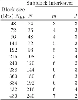
The six subblocks can be interleaved separately. The interleaving is performed in unit of bits. The sequence of interleaver output bits for each subblock can be generated by the procedure described below. The entire subblock of bits to be interleaved is written into an array at addresses from 0 to the number of the bits minus one (N − 1), and the interleaved bits are read out in a permuted order with the ith bit being read from the address ADi (i = 0, . . . , N − 1), as follows:

1. Determine the subblock interleaver parameters, m and J. Table 2.3 gives these pa-rameters.

Table 2.3: Parameters for the Subblock Interleavers Subblock interleaver Block size (bits) NEP N m J 48 24 3 3 72 36 4 3 96 48 4 3 144 72 5 3 192 96 5 3 216 108 5 4 240 120 6 2 288 144 6 3 360 180 6 3 384 192 6 3 432 216 6 4 480 240 7 2

3. Form a tentative output address Tk according to

Tk= 2m(k mod J) + BROm(bk/Jc) (2.1) where BROm(y) indicates the bit-reversed m-bit value of y (e.g. BRO3(6) = 3).

4. If Tk is less than N, ADi = Tk and increment i and k by 1. Otherwise, discard Tk and increment k only.

5. Repeat steps 3 and 4 until all N interleaver output addresses are obtained. Bit Grouping

The channel interleaver output sequence consists of the interleaved A and B subblock sequences, followed by a bit-by-bit multiplexed sequence of the interleaved Y 1 and Y 2 sub-block sequences, followed by a bit-by-bit multiplexed sequence of the interleaved W 1 and

Figure 2.9: Block diagram of CTC channel interleaving scheme (from [1]).

The bit-by-bit multiplexed sequence of interleaved Y 1 and Y 2 subblock sequences con-sists of the first output bit from the Y 1 subblock interleaver, the first output bit from the

Y 2 subblock interleaver, the second output bit from the Y 1 subblock interleaver, the second

output bit from the Y 2 subblock interleaver, etc. The bit-by-bit multiplexed sequence of interleaved W 1 and W 2 subblock sequences consists of the first output bit from the W 1 sub-block interleaver, the first output bit from the W 2 subsub-block interleaver, the second output bit from the W 1 subblock interleaver, the second output bit from the W 2 subblock inter-leaver, etc. Figure 2.9 shows the interleaving scheme. The order of bit grouping sequence is as follows: A0 0,A01,...,A0N −1,B00,B10,...,BN −10 , Y0 1,0,Y2,00 ,Y1,10 ,Y2,10 ,Y1,20 ,Y2,20 ,...,Y1,N −10 ,Y2,N −10 , W0 1,0,W2,00 ,W1,10 ,W2,10 ,W1,20 ,W2,20 ,...,W1,N −10 ,W2,N −10 .

Bit Selection

Lastly, bit selection is performed to generate the subpacket. The puncturing block is referred to as bit selection in the viewpoint of subpacket generation. The mother code is transmitted with one of the subpackets. The bits in a subpacket are formed by selecting specific sequences of bits from the interleaved CTC encoder output sequence. The resulting subpacket sequence is a binary sequence of bits for the modulator. The parameters for bit selection are listed below:

• k: the subpacket index when IR HARQ is enabled.

– When IR HARQ is not used, k=0 (for the first transmission and increases by one for the next subpacket).

– When there is more than one FEC block in a burst, the subpacket index for each FEC block shall be the same.

• NEP: the number of bits in the encoder packet (before encoding).

• NSCHk: the number of concatenated slots for the subpacket, as defined in [1, Table 569] for the non-HARQ and Chase HARQ CTC schemes.

• mk: the modulation order for the kth subpacket (mk=2 for QPSK, 4 for 16-QAM, and 6 for 64QAM).

• SP IDk: the subpacket ID for the kth subpacket (for the first subpacket, SP IDk=0=0).

Also, let the scrambled and selected bits be numbered from zero with the 0th bit being the first bit in the sequence. Then, the index of the ith bit for the kth subpacket shall be

where i = 0, . . . , Lk−1, Lk = 48·NSCHk·mk, and Fk= (SP IDk·Lk)mod(3·NEP). The NEP,

NSCHk, mk , and SP ID values are determined by the base station (BS) and can be inferred by the subscriber station (SS) through the allocation size in the DL-MAP and UL-MAP. The above bit selection makes the following possible.

• The first transmission includes the systematic part of the mother code. Thus it can

be used as the codeword for a burst where the HARQ is not applied or when Chase HARQ is applied.

• The location of the subpacket can be determined by the SP ID without the knowledge

of previous subpacket. This is a very important property for IR HARQ retransmission. Note that the optional IR HARQ is not considered in our research, so we bypass a detailed introduction of the IR HARQ mechanism.

2.1.7

Modulation [1]

After bit interleaving, the data bits are entered serially to the constellation map-per. Gray-mapped QPSK and 16-QAM are supported, whereas the support of 64-QAM is optional. The constellations as shown in Fig. 2.10 shall be normalized by multiplying the constellation points with the indicated factor c to achieve equal average power. The constellation-mapped data shall be subsequently modulated onto the allocated data carriers.

2.1.8

Demodulation for Bit-Interleaved Coded Modulation [3]

Let a[i] = aI[i] + jaQ[i] denote the QAM symbol transmitted via the ith sub-carrier of OFDMA symbol and {bI,1, · · · , bI,k, · · · , bI,t, bQ,1, · · · , bQ,k, · · · , bQ,t} be the corresponding bit sequence. Assuming that the ISI (inter–OFDMA symbol interference) and ICI (inter–carrier interference) are completely eliminated, we can write the received signal of the sub-carrier

Figure 2.10: QPSK, 16-QAM, and 64-QAM constellations (from [1]).

as

r[i] = Gch[i] · a[i] + w[i], (2.3)

where Gch[i] is the complex channel frequency response at the ith sub-carrier and w[i] is the complex additive white Gaussian noise (AWGN) with variance σ2 _{= N}

0. If the channel

estimate is error free, the output of the one-tap equalizer is given by

y[i] = a[i] + w[i]/Gch[i] = a[i] + w0[i], (2.4)

where w0_{[i] is still complex AWGN noise with variance σ}02_{(i) = σ}2_/|G

ch[i]|2.

According to the MAPSE (maximum a posterior sequence estimation) criterion, the following maximization should be performed to estimate the encoded bit sequence b:

ˆ

b = arg max

b P [b|r], (2.5)

where r is the received sequence of QAM signals. Assume that the transmitted symbols are equally distributed. Then the MAPSE criterion can be replaced by the ML (maximum

likelihood) criterion as:

ˆ

b = arg max

b P [r|b]. (2.6)

We further assume that Gch[i] is known to the receiver and that the transmitted bits are independent and identically distributed (i.i.d.).

For each in-phase or quadrature bit (i.e., bI,k or bQ,k), two metrics can be derived cor-responding to the two possible values 0 and 1, respectively. For bit bI,k, first the QAM constellation is split into two partitions of complex symbols, namely S_I,k(0) comprising the symbols with a “0” in position (I, k) and S_I,k(1), which is complementary. Then the two metrics are obtained by

m0

c(bI,k) = X α∈S_I,k(c)

log p(r[i]|a[i] = α) ≈ max α∈S(c)_I,k

log p(r[i]|a[i] = α), c = 0, 1. (2.7) Since the conditional pdf of r[i] is complex Gaussian as

p(r[i]|a[i] = α) = √1 2πσ exp{− 1 2 |r[i] − Gch[i]α|2 σ2 } (2.8)

and r[i] = Gch[i] · y[i], the metrics defined in (2.32) are equivalent to

mc(bI,k) = |Gch[i]|2· min α∈S_I,k(c)

|y[i] − α|2. (2.9)

Finally, these metrics are de-interleaved, i.e., each couple (m0, m1) is assigned to the bit

position in the decoded sequence according to the de-interleaver map, and fed to the Viterbi decoder which selects the binary sequence with the smallest cumulative sum of metrics. We name this method Method-ML in the following discussion.

From the concept of log-likelihood ratio (LLR), a method named Method-LLR is proposed in [3] to reduce the complexity of Method-ML. It defines LLR(bI,k) as

LLR(bI,k) , |Gch[i]|2 4 { min_α∈S(0) I,k |y[i] − α|2_{− min} α∈S_I,k(1) |y[i] − α|2_} , (m0(bI,k) − m1(bI,k))/4 , |Gch[i]|2· DI,k. (2.10)

Table 2.4: Bit Metric for Method-ML and Method-LLR Method-ML Method-LLR Bit metric (decided “0”) m0 [1₄(m0− m1) + 1)]2

Bit metric (decided “1”) m1 [1₄(m0− m1) − 1)]2

The quadrature part is similarly defined. The metrics sent to the Viterbi decoder in the two methods are defined in Table 2.4. Note that the difference between the bit metrics for the decided “0” and “1” is the same for the two methods, namely ±(m0− m1). Thus the

decoded bit sequence will be the same for the two methods.

In Method-LLR, only (m0− m1)/4 is sent to the de-interleaver while in Method-ML, both

m0 and m1 are sent. Besides, we can reduce (m0− m1)/4 = |Gch[i]|2· DI,k to a simple form constituting of yI[i] itself because Gray coding is used in the constellation map of M-ary QAM modulation in IEEE 802.16e.

Figure 2.11 shows the partitions of (S_I,k(0), S_I,k(1)) for the generic bit bI,k in the case of 16-QAM. As a consequence, DI,k = 1 4{ min_α∈S(0) I,k |y[i] − α|2_{− min} α∈S_I,k(1) |y[i] − α|2_}

can be simplified as follows.

DI,1 =

  

−yI[i], |yI(i)| ≤ 2

−2(yI[i] − 1), yI(i) > 2

−2(yI[i] + 1), yI(i) < 2  

 ∼= −yI[i], (2.11)

DI,2 = |yI[i]| − 2. (2.12) The same observation holds for QPSK and 64-QAM constellations. For QPSK, DI = −yI[i].

S_I,10 S_I,11 _S1 _S1 I,2 S0 I,2 I,2 x x −1 1 3 −3 (10) (00) (01) I −1 1 3 −3(11) (10) (00) (01) (11) BI,1 BI,2 Q Q I

Figure 2.11: Metric partitions of the 16-QAM constellation (from [3]). For 64-QAM, DI,1 =                   

−yI[i], |yI[i]| ≤ 2

−2(yI[i] − 1), 2 < yI[i] ≤ 4

−3(yI[i] − 2), 4 < yI[i] ≤ 6

−4(yI[i] − 3), yI[i] > 6

−2(yI[i] + 1), −4 ≤ yI[i] < −2

−3(yI[i] + 2), −6 ≤ yI[i] < −4

−4(yI[i] + 3), yI[i] < −6

                   ∼ = −yI[i], (2.13) DI,2 =   

2(|yI[i]| − 3), |yI[i]| ≤ 2

−4 + |yI[i]|, 2 < |yI[i]| ≤ 6

2(|yI[i]| − 5), |yI[i]| > 6

 

 ∼= −4 + |yI[i]|, (2.14)

DI,3 =

½

−|yI[i]| + 2, |yI[i]| ≤ 4

|yI[i]| − 6, |yI[i]| > 4 ¾

= ||yI[i]| − 4| − 2. (2.15)

2.2

Decoding of CTC

2.2.1

The Turbo Decoding Algorithm [5]

A key in turbo codes is the iterative decoding algorithm. In iterative decoding, the decoders for the constituent encoders take turns operating on the received data.

Each decoder produces an estimate of the probabilities of the transmitted symbols; there-fore, the decoders are soft output decoders. Probabilities of the symbols from one decoder, known as extrinsic probabilities, are interleaved and passed to the other decoder, where

Figure 2.12: Block diagram of a turbo decoder (from [5]).

they are used as prior probabilities for the other decoder. The decoder thus passes proba-bilities back and forth between the decoders, with each decoder combining the evidence it receives from the incoming prior probabilities with the parity information provided by the code. After some number of iterations, hopefully the decoder converges to an estimate of the transmitted codeword. Since the output of one decoder is fed to the input of the next decoder, the decoding algorithm is called a turbo decoder, for it is reminiscent of turbo charging an automobile engine using engine-heated air at the air intake. Thus it is not really the code which is “turbo,” but rather the decoding algorithm which is “turbo.” The general operation of the turbo decoding algorithm is shown in Fig. 2.12.

The MAP Decoding Algorithm [5], [7]

One maximum a posteriori (MAP) decoding algorithm particularly suitable for estimat-ing bit and/or state probabilities for a finite-state Markov system is the BCJR algorithm, named after Bahl, Cock, Jelinek, and Raviv who originally proposed it in 1974 [6]. While this algorithm has been known for some time, it was not extensively used for the decoding of convolutional codes because of the availability of a lower complexity Viterbi algorithm (for maximum-likelihood decoding of convolutional codes).

the conventional Viterbi algorithm computes hard decisions by outputting a single overall decision of the entire sequence of bits (or codeword) at the end, without providing the reliability of the decoder decisions on individual bits. Furthermore, the branch metric is based upon log likelihood values; no prior information is incorporated into the decoding process. The BCJR algorithm, on the other hand, computes soft outputs in the form of posterior probabilities for each message bit. While the Viterbi algorithm produces the maximum likelihood message sequence (or codeword), the BCJR algorithm produces the a posteriori most likely sequence of message bits, where the sequence of bits may not correspond to a continuous path through the trellis. The BCJR algorithm is a soft-input soft-output decoder that can be used directly in turbo decoding whereas the conventional Viterbi algorithm cannot without some modification to yield the required soft output. The BCJR algorithm for MAP decoding of convolutional codes consists of the following steps:

• Compute branch metric γ.

• Compute forward state metric α. • Compute backward state metric β.

• Compute extrinsic log likelihood ratio Le.

A more detailed understanding can be gained from [5].

2.2.2

Decoding Rule for CRSC Codes with Non-binary Trellis [8]

The trellis of a double-binary feedback convolutional encoder has the structure shown in Fig. 2.13. The goal of the MAP algorithm is to provide us with

Li(dk) = ln Pr[dk = i|Observation] Pr[dk= 0|Observation] = ln P_(Sk−1,Sk) dk=i p(Sk−1, Sk, {yk}) P_(Sk−1,Sk) dk=0 p(Sk−1, Sk, {yk}) , i = 1, 2, 3, (2.16)

Figure 2.13: CTC trellis structure of duo-binary convolutional code with feedback encoder (from [8]).

where yk is the received sample at time k. The index pair (Sk−1, Sk) determines the infor-mation symbol (bit couple) dk and the coded symbol xk from time k − 1 to time k where

dk is in GF(22) with elements {0,1,2,3}. The sum of the joint probabilities p(Sk−1, Sk, {yk}) in the numerator or in the denominator of (2.16) is taken over all path labeled with dk = i,

i = 0, 1, 2, 3, where we have used decimal notation for dk instead of binary for convenience.

With a memoryless transmission channel, the joint probability p(Sk−1, Sk, {yk}) can be writ-ten as the product of three independent probabilities

p(Sk−1, Sk, {yk}) = p(Sk−1, yj<k) · p(Sk, yk|Sk−1) · p(yj>k, Sk)

, αk−1(Sk−1) · γk(Sk−1, Sk) · βk(Sk) (2.17) where yj<k denotes the sequence of received symbols yj from the beginning of the trellis up to time k − 1 and yj>k is the corresponding sequence from time k + 1 up to the end of the

trellis. The forward recursion of the MAP algorithm yields

αk(Sk) =

X Sk−1

αk−1(Sk−1) · γk(Sk−1, Sk). (2.18) The backward recursion yields

βk−1(Sk−1) =

X Sk

γk(Sk−1, Sk) · βk(Sk). (2.19) When a transition between Sk−1 and Sk exists, the branch transition probability is given by

γk(Sk−1, Sk) = p(Sk, yk|Sk−1)

= p(Sk|Sk−1) · p(yk|Sk−1, Sk)

= P (dk) · p(yk|dk). (2.20) Let the natural logarithm of the branch transition probability metric be

Γk(Sk−1, Sk) = ln γk(Sk−1, Sk) (2.21) and the natural logarithms of αk(Sk) and βk(Sk) be

Ak(Sk) = ln αk(Sk) = lnX Sk−1 eAk−1(Sk−1)+Γk(Sk−1,Sk), (2.22) Bk−1(Sk−1) = ln βk−1(Sk−1) = lnX Sk eΓk(Sk−1,Sk)+Bk(Sk)_{. (2.23)}

Then the log-likelihood ratios (2.16) for i = 1, 2, 3 are given by

Li(dk) = ln P_(Sk−1,Sk) dk=i p(Sk−1, Sk, {yk}) P_(Sk−1,Sk) dk=0 p(Sk−1, Sk, {yk}) = ln P_(Sk−1,Sk) dk=i αk−1(Sk−1) · γ i k(Sk−1, Sk) · βk(Sk) P_(Sk−1,Sk) dk=0 αk−1(Sk−1) · γ 0 k(Sk−1, Sk) · βk(Sk) = ln P_(Sk−1,Sk) dk=i e Ak−1(Sk−1)+Γik(Sk−1,Sk)+Bk(Sk) P_(Sk−1,Sk) dk=0 e Ak−1(Sk−1)+Γ0k(Sk−1,Sk)+Bk(Sk) . (2.24)

2.2.3

Simplified Max-Log-MAP Algorithm for Double-Binary CTC

[8]

Implementing (2.24) in hardware is difficult and complex. It is also relatively compli-cated to implement it in DSP software. We consider the suboptimal max-log-MAP algorithm for double binary convolutional turbo codes. First, from (2.20) and (2.21),

Γk(Sk−1, Sk) = ln γk(Sk−1, Sk)

= ln[p(yk|dk) · P (dk)]. (2.25) The distribution of the received symbols is given by, for i = 0, 1, 2, 3,

p(yk|dk = i) = p(yks|xsk(i)) · p(ykp|xpk(i, Sk−1, Sk)) = 1 π · N0 e−EsN0[(y s,I k −x s,I k (i))2+(y s,Q k −x s,Q k (i))2] · 1 π · N0 e−EsN0[(y p,I k −x p,I k (i,Sk−1,Sk))2+(y p,Q k −x p,Q k (i,Sk−1,Sk))2] = Ck· e0.5·Lc·[y s,I k ·x s,I k (i)+y s,Q k ·x s,Q k (i)+y p,I k ·x p,I k (i,Sk−1,Sk)+ykp,Q·x p,Q k (i,Sk−1,Sk)] where ys

kand ypkrepresent the received systematic and parity symbols, respectively, ys,Ik , yks,Q,

y_kp,I, and y_kp,Qrepresent the received bit values transmitted through the I and Q channels, re-spectively, Lc = 4 · (fading factor) · (code rate) · E_Nb₀ represent the channel reliability, and

Ck = (_π·N1₀)2e− Es N0[(y s,I k )2+(x s,I k (i))2+(y s,Q k )2+(x s,Q k (i))2+(y p,I k )2+(x p,I k (i,Sk−1,Sk))2+(ykp,Q)2+(x p,Q k (i,Sk−1,Sk))2]_. Hence, Γk(Sk−1, Sk) = ln[p(yk|dk) · P (dk)] = 0.5 · Lc· [yks,I· x s,I k (i) + y s,Q k · x s,Q k (i) + y p,I k · x p,I k (i, Sk−1, Sk) +y_kp,Q· xp,Q_k (i, Sk−1, Sk)] + ln P (dk) + K (2.26)

where the constant K includes the constants and common terms that are cancelled in com-parisons at later stages. Note that

Ak(Sk) = ln X Sk−1 eAk−1(Sk−1)+Γk(Sk−1,Sk) ≈ max Sk−1 [Ak−1(Sk−1) + Γk(Sk−1, Sk)], (2.27) Bk−1(Sk−1) = ln X Sk eΓk(Sk−1,Sk)+Bk(Sk) ≈ max Sk [Γk(Sk−1, Sk) + Bk(Sk)]. (2.28) The above can be derived by considering the Jacobian logarithm [5], i.e.,

ln(eL1+ eL2) = max(L1, L2) + ln(1 + e−|L1−L2|). (2.29)

If the correction term (i.e., the second right-hand-side [RHS] term) is omitted and only the max term is retained, we obtain the above max-function (max-log-MAP) approximation. For iterative decoding of circular trellis, tail-biting gives

A0(S0) = AN(SN) ∀S0, (2.30)

BN(SN) = B0(S0) ∀SN. (2.31) As a result, the log-likelihood ratios in (2.24) reduce to

Li(dk) ≈ max (Sk−1,Sk) [Ak−1(Sk−1) + Γik(Sk−1, Sk) + Bk(Sk)] − max (Sk−1,Sk) [Ak−1(Sk−1) + Γ0k(Sk−1, Sk) + Bk(Sk)]. (2.32) We omit the detailed mathematical derivation for separating the log-likelihood ratios into intrinsic (prior information), systematic and extrinsic information. The interested reader may refer to [8]. It turns out that the extrinsic information can be expressed as

L_ie( ˆdk) = Li( ˆdk) − 0.5 · [y_ks,I · xs,I_k (i) + y_ks,Q· xs,Q_k (i)]

+0.5 · [ys,I_k · xs,I_k (0) + y_ks,Q· xs,Q_k (0)] − ln P [dk= i]

P [dk = 0]

The extrinsic information of the next decoder is computed from the prior information of previous decoder as La i(dk) = ln P [dk = i] P [dk= 0] (2.34) where i = 0, 1, 2, 3. Since P [dk = 01] = eL a 1(dk)_{· P [d} k= 00], P [dk = 10] = eL a 2(dk)· P [d k= 00], P [dk = 11] = eL a 3(dk)_{· P [d} k= 00], and P [dk = 00] + P [dk = 01] + P [dk = 10] + P [dk = 11] = 1, (2.35) we have P [dk = 00] = 1 1 + eLa 1(dk)+ eLa2(dk)+ eLa3(dk), P [dk = 01] = La 1(dk) 1 + eLa 1(dk)+ eLa2(dk)+ eLa3(dk), P [dk = 10] = La 2(dk) 1 + eLa 1(dk)+ eLa2(dk)+ eLa3(dk), P [dk = 11] = La 3(dk) 1 + eLa 1(dk)+ eLa2(dk)+ eLa3(dk). (2.36)

Using max-function approximation yields

ln P [dk= 00] = − max[0, La1(dk), L2a(dk), La3(dk)],

ln P [dk= 01] = La1(dk) − max[0, La1(dk), La2(dk), La3(dk)], ln P [dk= 10] = La2(dk) − max[0, La1(dk), La2(dk), La3(dk)],

ln P [dk= 11] = La3(dk) − max[0, La1(dk), La2(dk), La3(dk)]. (2.37)

Assuming equally likely symbols initially, we have

A0(S0) = 0 ∀S0, (2.38)

BN(SN) = 0 ∀SN, (2.39)

La

i(dk) = 0 ∀i, dk. (2.40) After sufficient decoding iterations, the decisions are made according to

ˆ dk =        01, if L( ˆdk) = La1(dk) and La1(dk) > 0, 10, if L( ˆdk) = La2(dk) and La2(dk) > 0, 11, if L( ˆdk) = La3(dk) and La3(dk) > 0, 00, else, (2.41) where L( ˆdk) = max[La1(dk), La2(dk), La3(dk)].

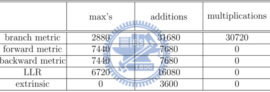
This above algorithm has been known as the max-log-MAP algorithm which only uses the max functions to compute log-likelihood ratios. But coming with the approximation to reducing log-likelihood ratios is some performance degradation. Table 2.5 shows the complexity analysis. We will discuss later the simulation results and the speed of our DSP implementation.

Table 2.5: Amount of Additions, Multiplications and Max Operations for Soft-Output De-coding of One Component Code Once, Where Number of Information Bits = 480

max’s additions multiplications branch metric 2880 31680 30720 forward metric 7440 7680 0 backward metric 7440 7680 0 LLR 6720 16080 0 extrinsic 0 3600 0

Chapter 3

DSP Implementation Environment

In this chapter, our discussion will concentrate on the DSP system development en-vironment, DSP chip and its features because our implementation is software-based on the DSP. The software development tool, Code Composer Studio (CCS), is also introduced.

3.1

The DSP Board [12]

The DSP card used in our implementation is Sundance’s SMT395 as shown in Fig. 3.1 [11]. It houses a 1 GHz 64-bit TMS320C6416T DSP of TI . The SMT395 is supported by TI’s Code Composer Studio and the 3L Diamond to enable multi-DSP systems with minimum development efforts by the programmers.

Features of the SMT395 board include:

• 1 GHz TMS320C6416T fixed-point DSP processor with L1 and L2 cache that has 8000

MIPS peak DSP performance.

• Xlilinx Virtex II Pro FPGA XC2VP30-6 in FF896 package. • 256 Mbytes of SDRAM at 133MHz.

Figure 3.1: Sundance’s SMT395 module (from [11]).

• Two Sundance High-speed Bus (50,100 or 200 MHz) ports at 32 bits width. • 8-Mbyte flash ROM for configuration and booting.

3.2

The DSP Chip [12]

The TMS320C64x DSP is a fixed-point DSP in the TMS320C64x series of the TMS320C6000 DSP platform family. The TMS320C64x device use the very-long-instruction-word (VLIW) architecture developed by TI. The C6416 device has two high-performance embedded copro-cessors, Viterbi Decoder Coprocessor (VCP) and Turbo Decoder Coprocessor (TCP) that can significantly speed up channel-decoding operations on chip. However the TCP is de-signed appropriately for the 3GPP standard and its parameter setting cannot be used to the CTC in 802.16e. Therefore, we cannot employ the TCP in our implementation.

The C64x core CPU consists of 64 general-purpose 32-bits registers and 8 function units. Features of C6000 devices include:

– Execute up to eight instructions per cycle.

– Allow designers to develop highly effective RSIC-like code for fast development time.

• Instruction packing:

– Gives code size equivalence for eight instructions executed serially or in parallel. – Reduces code size, program fetches, and power consumption.

• Conditional execution of all instructions:

– Reduces costly branching.

– Increases parallelism for higher sustained performance.

• Efficient code execution on independent functional units:

– Efficient C compiler on DSP benchmark suite.

– Assembly optimizer for fast development and improved parallelization.

• 8/16/35/64-bit data support, providing efficient memory support for a variety of

ap-plication.

• 40-bit arithmetic options add extra precision for applications requiring it. • Saturation and normalization provide support for key arithmetic operations.

• Field manipulation and instruction extract, set, clear, and counting support common

operation found in control and data manipulation application.

• 32 × 32-bit integer multiply with 32- or 64-bit result.

• Each multiplier can perform two 16x16 bits or four 8x8 bits multiplies every clock

cycle.

• Quad 8-bit and dual 16-bit instructions set extensions with data flow support.

• Special communication-specific instruction have been added to address common

oper-ations inerror-correcting codes.

• Bit count and rotate hardware extends support for bit-level algorithms.

In the following subsections, two major parts of TMS320C64x DSP are introduced re-spectively. They are the central processing unit and memory .

3.2.1

Central Processing Unit [12]

The C64x DSP core contains 64 32-bit general purpose registers, program fetch unit, instruction decode unit, two data paths each with four function units, control register, control logic, test unit, emulation logic and interrupt logic. The program fetch, instruction fetch and instruction decode units can arrange eight 32-bit instructions to the eight function units every CPU clock cycle. The processing of instructions occurs in each of the two data paths (A and B) shown in Fig. 3.2, each of which contains four functional units and one register file. The four functional units are: one unit for multiplier operations (.M), one for arithmetic and logic operation (L.), one for branch, byte shifts, and arithmetic operation (.S), and one for linear and circular address calculation to load and store with external memory operations (.D). The details of the function units are described in Table 3.1.

Each register file consists of 32 × 32-bit registers. Each function unit in the two sets of four functional units reads and writes directly within its own data path. That is, functional units .L1, .S1, .M1 and .D1 can only write to register file A. The same holds for register file B. However, two cross-paths (1X and 2X) allow functional units from one data path to

Table 3.1: Functional Units and Operations Performed [12] Function

Unit Operations

.L unit (.L1, .L2) 32/40-bit arithmetic and compare operations 32-bit logical operations

Leftmost 1 or 0 counting for 32 bit Normalization count for 32 and 40 bits Byte shifts

Data packing/unpacking 5-bit constant generation

Dual 16-bit and Quad 8-bit arithmetic operations Dual 16-bit and Quad 8-bit min/max operations .S unit (.S1, .S2) 32-bit arithmetic operations

32/40-bit shifts and 32-bit bit-field operations 32-bit logical operations

Branches

constant generation

Register transfers to /from control register file (.S2 only) Byte shifts

Data packing/unpacking

Dual 16-bit and Quad 8-bit compare operations

Dual 16-bit and Quad 8aturated arithmetic operations .M unit (.M1, .M2) 16 × 16 multiply

16 × 32 multiply operations

Dual 16 × 16 and Quad 8 × 8 multiply operations Dual 16 × 16 multiply with add/substract operations Quad 8 × 8 multiply with add operations

Bit expansion

Bit interleaving/de-interleaving Variable shift operations

Rotation

Galois Field Multiply

.D unit (.D1, .D2) 32-bit add, subtract, linear and circular address calculation Loads and store with 5-bit constant offset

Loads and stores with 15-bit constant offset (.D2 only) Loads and stores doubles words with 5-bit constant Loads and store non-aligned word and double words 5-bit constant generation

Figure 3.2: Functional block and CPU (DSP core) diagram [13].

access a 32-operand the opposite-side register file. The cross path 1X allows data path A to read its source from register file B. The cross path 2X allows data path B to read its source from register file A. In the C64x, CPU pipelines data-cross-path accesses over multiple clock cycles. This allows the same register to be used as a data-cross-path operand by multiply functional units in the same execute packet.

3.2.2

Memory [14]

Internal Memory

The C64x DSP chip has a 32-bit, byte-addressable address space. Internal (on-chip) memory is organized in separate data and program spaces. When off-chip memory is used, these spaces are unified on most devices to a single memory space via the external memory interface (EMIF). The C64x has two 64-bit internal ports to access internal data memory and a single internal port to access internal program memory, with an instruction-fetch width of 256 bits.

Memory Options

The C64x DSP Chip also provides a variety of memory options:

• Program cache. • 2-level caches.

• 32-bit external memory interface supports SDRAM, SBRAM, SRAM,

and other asynchronous memories for a broad range of external memory requirements and maximum system performance.

Cache Memory

The C64x memory architecture consist of a two-level internal cache-based memory ar-chitecture plus external memory. Level cache is split into program (L1P) and data (L1D) caches. The C64x memory architecture is shown in Fig. 3.3. On C64x devices, each L1 cache is 16KB. All caches and data paths are automatically managed by cache controller. Level 1 cache is accessed by the CPU without stalls. Level 2 cache is configurable and can be split

Figure 3.3: C64x cache memory architecture [14].

into L2 SRAM (addressable on-chip memory) and L2 cache for caching external memory locations. On a C6416 DSP, the size of L2 cache is 1 MB, and the external memory can be several Mbytes large. More detailed introduction to the cache system can be found in [14].

3.3

TI’s Code Development Environment [15]

TI provides a useful GUI development interface to DSP users for developing and de-bugging their projects: Code Composer Studio (CCS). The CCS development tools are a key element of the DSP software and development tools from Texas Instruments. The fully integrated development environment include real-time analysis capabilities, easy to use debugger, C/C++ compiler, assembler, linker, editor, visual project manager, simulators, XDS560 and XDS510 emulation drivers, and DSP/BIOS support.

Some of CCS’s fully integrated host tools include:

• Integrated visual project manager with source control interface, multi-project support

and the ability to handle thousands of project files.

• Source code debugger common interface for both simulator and emulator targets;

– C/C++/assembly language support. – Simple breakpoint.

– Advanced watch window. – Symbol browser.

• DSP/BIOS host tooling support (configure, real-time analysis and debugger). • Data transfer for real time data exchange between host and target.

• Profiler to understand code performance.

CCS also delivers foundation software consisting of:

• DSP/BIOS kernel for the TMS320C6000 DSPs:

– Pre-emptive multi-threading. – Inter-thread communication. – Interrupt handling.

• TMS320 DSP Algorithm Standard to enable software reuse.

• Chip Support Library (CSL) simplify device configuration. CSL provides C-program

• DSP library for optimum DSP functionality. The library includes many C-callable,

assembly-optimized, general-purpose signal-processing and image/video processing rou-tines. These routines are typically used in computationally intensive real-time appli-cations where optimal execution speed is critical.

3.4

Code Development Flow [17]

The recommended code development flow involves utilizing the C6000 code generation tools to aid in optimization rather than forcing the programmer to code by hand in assembly. Hence the programmer may let the compiler do all the laborious work of instruction selection, parallelizing, pipelining, and register allocation. This simplifies the maintenance of the code, as everything resides in a C framework that is simple to maintain, support, and upgrade. Fig. 3.4 illustrates the three phases in the code development flow. Because phase 3 is usually too detailed and time consuming, most of the time we will not go into phase 3 to write linear assembly code unless the software pipelining efficiency is too bad or the resource allocation is too unbalanced.

3.5

Code Optimization on TI DSP Platform

In this section, we describe several methods that can accelerate our code and reduce the execution time on the C64x DSP. First, we introduce two techniques that can be used to analyze the performance of specific code regions:

• Use the clock( ) and printf( ) functions in C/C++ to time and display the performance

of specific code regions. Use the stand-alone simulator (load6x) to run the code for this purpose.

code with the -mg option and executing load6x with the -g option. Then enable the clock and use profile points and the RUN command in the Code Composer debugger to track the number of CPU clock cycles consumed by a particular section of code. Use “View Statistics” to view the number of cycles consumed.

Usually, we use the second technique above to analyze the C code performance. The feedback of the optimization result can be obtained with the -mw option. It shows some important results of the assembly optimizer for each code section. We take these results into consideration in improving the computational speed of certain loops in our program.

3.5.1

Compiler Optimization Options [17]

In this subsection, we introduce the compiler options that control the operation of the compiler. The CCS compiler offers high-level language support by transforming C/C++ code into more efficient assembly language source code. The compiler options can be used to optimize the code size or the executing performance.

The major compiler options we use are -o3, -k, -pm -op2, -mh<n>, -mw, and -mi.

• -on: The “n” denotes the level of optimization (0, 1, 2, and 3), which controls the type

and degree of optimization.

– -o3: highest level optimization, whose main features are:

∗ Performs software pipelining.

∗ Performs loop optimizations, and loop unrolling. ∗ Removes all functions that are never called.

∗ Reorders function declarations so that the attributes of called functions are

∗ Propagates arguments into function bodies when all calls pass the same value

in the same argument position.

∗ Identifies file-level variable characteristics.

• -k: Keep the assembly file to analyze the compiler feedback.

• -pm -op2: In the CCS compiler option, -pm and -op2 are combined into one option.

– -pm: Gives the compiler global access to the whole program or module and allows it to be more aggressive in ruling out dependencies.

– -op2: Specifies that the module contains no functions or variables that are called or modified from outside the source code provided to the compiler. This improves variable analysis and allowed assumptions.

• -mh<n>: Allows speculative execution. The appropriate amount of padding, n, must

be available in data memory to insure correct execution. This is normally not a problem but must be adhered to.

• -mw: Produce additional compiler feedback. This option has no performance or code

size impact.

• -mi: Describes the interrupt threshold to the compiler. If the compiler knows that no

interrupts will occur in the code, it can avoid enabling and disabling interrupts before and after software-pipelined loops for improvement in code size and performance. In addition, there is potential for performance improvement where interrupt registers may be utilized in high register pressure loops.