Probability density of nonlinear phase noise
Keang-Po HoStrataLight Communications, Campbell, California 95008, and Graduate Institute of Communications Engineering, College of Electrical Engineering and Computer Science, National Taiwan University, Taipei, Taiwan
Received January 9, 2003; revised manuscript received April 25, 2003
The probability density of nonlinear phase noise, often called the Gordon–Mollenauer effect, is derived ana-lytically. The nonlinear phase noise can be accurately modeled as the summation of a Gaussian random vari-able and a noncentral chi-square random varivari-able with two degrees of freedom. Using the received intensity to correct for the phase noise, the residual nonlinear phase noise can be modeled as the summation of a Gauss-ian random variable and the difference of two noncentral chi-square random variables with two degrees of freedom. The residual nonlinear phase noise can be approximated by Gaussian distribution better than the nonlinear phase noise without correction. © 2003 Optical Society of America
OCIS codes: 190.3270, 060.5060, 060.1660, 190.4370.
1. INTRODUCTION
Gordon and Mollenauer1 showed that, when optical am-plifiers are used to compensate for fiber loss, the interac-tion of amplifier noise and the fiber Kerr effect causes phase noise, often called the Gordon–Mollenauer effect or nonlinear phase noise. By broadening the signal linewidth,2 nonlinear phase noise degrades both phase-shifted keying and differential phase-shift keying sys-tems, which have renewed attention recently.3–5 Be-cause the nonlinear phase noise is correlated with the received intensity, the received intensity can be used to correct the nonlinear phase noise.6–8 The transmission distance can be doubled if the nonlinear phase noise is the dominant impairment.6,8
Usually, the performance of the system is estimated based on the variance of the nonlinear phase noise.1,6–8
The probability-density function (pdf) is necessary to bet-ter understand the system and evaluates the system per-formance. This paper provides an analytical expression of the pdf for the nonlinear phase noise with6–8 and without1 the correction by the received intensity. The characteristic functions are first derived analytically, and the pdf ’s are the inverse Fourier transform of the charac-teristic functions.
2. PROBABILITY-DENSITY FUNCTION
For simplicity and without loss of generality, assume that the total nonlinear phase noise is1,6,8
NL⫽ 兩A ⫹ n1兩2⫹ 兩A ⫹ n1⫹ n2兩2
⫹ ¯ ⫹ 兩A ⫹ n1⫹¯ ⫹ nN兩2, (1)
where A is a real number representing the amplitude of the transmitted signal, nk⫽ xk⫹ iyk, k⫽ 1,..., N, are
the optical amplifier noise introduced into the system at the kth fiber span, and nkare independent identically
dis-tributed complex zero-mean circular Gaussian random variables with E兵xk2其⫽ E兵yk2其⫽ E兵兩nk兩2其/2⫽ 2, where
2 is the noise variance per dimension per span and E兵 其 denotes expectation. The product of fiber
nonlin-ear coefficient and the effective length per span ␥Leffis
ignored in Eq. (1) for simplicity.1,6,8 The random variable of Eq. (1) is a quadratic form of complex random variables9; in order to find a simplified representation, we derive its characteristic function here.
First, we consider the random variable of 1⫽ 兩A ⫹ x1兩2⫹ 兩A ⫹ x1⫹ x2兩2
⫹¯ ⫹ 兩A ⫹ x1⫹¯ ⫹ xN兩2. (2)
The overall nonlinear phase noise of Eq. (1) isNL⫽1
⫹ 2, where
2⫽ y12⫹ 兩 y1⫹ y2兩2⫹¯ ⫹ 兩 y1⫹¯ ⫹ yN兩2 (3)
is independent of 1 and has a pdf equal to that of 1
when A ⫽ 0. The random variable of Eq. (2) can be ex-pressed as
1⫽ NA2⫹ 2AwTx⫹ xTCx, (4)
where w⫽兵N, N⫺ 1,..., 2, 1其T, x⫽兵x
1, x2,..., xN其T,
and the covariance matrixC ⫽ MTM with
M ⫽
冋
1 0 0 ¯ 0 1 1 0 ¯ 0 1 1 1 ¯ 0 ] ] ] ] 1 1 1 ¯ 1册
. (5)The pdf of x is (22)⫺N/2exp(⫺xTx/22). The
char-acteristic function of1,⌿1() ⫽ E兵exp( j1)其, is
⌿1共兲 ⫽
exp共 jNA2兲
共22兲N/2
冕
exp共2jAwTx⫺ xT⌫x兲dx,
(6) where⌫ ⫽ I/(22) ⫺ jC and I is an N ⫻ N identity ma-trix. Using the relationship of
xT⌫x ⫺ 2jAwTx⫽ 共x ⫺ jA⌫⫺1w兲T⌫共x ⫺ jA⌫⫺1w兲
⫹2A2wT⌫⫺1w, (7) 0740-3224/2003/091875-05$15.00 © 2003 Optical Society of America
with some algebra, the characteristic function of Eq. (6) is ⌿1共兲 ⫽
exp共 jNA2⫺2A2wT⌫⫺1w兲
共22兲N/2det共⌫兲1/2 , (8)
where det[ ] is the determinant of a matrix. The char-acteristic function of Eq. (8) is
⌿1共兲 ⫽
exp关 jNA2⫺ 222A2wT共I ⫺ 2j2C兲⫺1w兴
det共I ⫺ 2j2C兲1/2 .
(9) Substituting A ⫽ 0 into Eq. (9), the characteristic func-tion of2 is⌿2() ⫽ det关I ⫺ 2j 2C兴⫺1/2. The charac-teristic function ofNLis⌿NL() ⫽ ⌿1()⌿2(), or ⌿NL共兲 ⫽ exp关 jNA 2⫺ 222A2wT共I ⫺ 2j2C兲⫺1w兴 det共I ⫺ 2j2C兲 . (10)
If the covariance matrix C has eigenvalues and eigen-vectors ofk, vk, k⫽ 1, 2,..., N, respectively, the
charac-teristic function of Eq. (10) becomes
⌿NL共兲 ⫽ exp
冋
jNA2⫺ 222A2兺
k⫽1 N 共vk Tw兲2 1 ⫺ 2j2 k册
兿
k⫽1 N 共1 ⫺ 2j2 k兲 (11) and can be rewritten to⌿NL共兲 ⫽
兿
k⫽1 N 1 1 ⫺ 2j2 k exp冋
jA2共v k Tw兲2/ k 1 ⫺ 2j2 k册
. (12)From the characteristic function of Eq. (12), the random variable ofNL[Eq. (1)] is the summation of N
indepen-dently distributed noncentral chi-square (2) random
variables with two degrees of freedom.10 The
eigenval-ues of the covariance matrix ofC are all positive and mul-tiply to unity.
Without going into detail, the matrix
C⫺1⫽
冋
1 ⫺ 1 0 ¯ 0 0 ⫺1 2 ⫺ 1 ¯ 0 0 0 ⫺ 1 2 ¯ 0 0 ] ] ] ] ] 0 0 0 ¯ ⫺ 1 2册
(13)is approximately a Toeplitz matrix for the series of 2,⫺1, 0,... For large N, the eigenvalues of the covariance ma-trix ofC are asymptotically equal to11
1 k ⬇ 2
再
1 ⫺ cos冋
共2k ⫹ 1兲 2N册冎
⫽ 4 sin2冋
共2k ⫺ 1兲 4N册
, k⫽ 1,..., N. (14) The values of Eq. (14) are the discrete Fourier transform of each row of the matrixC⫺1.With the correction of phase noise using received intensity,6–8the residual nonlinear phase noise is
RES⫽ 兩A ⫹ n1兩2⫹ 兩A ⫹ n1⫹ n2兩2
⫹ ¯ ⫹ 兩A ⫹ n1⫹¯ ⫹ nN⫺1兩2
⫺ 共␣opt⫺ 1兲兩A ⫹ n1⫹¯ ⫹ nN兩2. (15)
As from the appendix, ␣opt⬇ (N ⫹ 1)/2 is the optimal
scale factor to correct the nonlinear phase noise of Eq. (1) using the received intensity of 兩A⫹ n1⫹¯ ⫹ nN兩2.
The random variable corresponding to 1 [Eq. (4)]
be-comes
共N ⫺␣opt兲A2⫹ 2AwrTx⫹ xTCrx, (16)
where wr⫽ w ⫺␣opt⫻兵1, 1,..., 1其Tand
Cr⫽ 共M ⫺ L兲T共M ⫺ L兲 ⫺ 共␣opt⫺ 1兲LTL, (17) where L ⫽
冋
0 0 ¯ 0 0 ] ] ] ] 0 0 ¯ 0 0 1 1 ¯ 1 1册
. (18)Following the procedure from Eqs. (4) to (10), the char-acteristic function ofRESis
The characteristic functions ofRESin the form of
eigen-values and eigenvectors are similar to those of Eqs. (11) and (12). The characteristic functions ofRES have the
same expression as Eq. (12) using a new set of eigenval-ues and eigenvectors of the covariance matrixCrand the
vector of wr.
Except for the first and last rows, the matrixCr⫺1is also approximately a Toeplitz matrix for the series of 2, ⫺1, 0,... For large N, the eigenvalues ofCrare asymptotically
equal to 1 k ⬇ 4 sin2
冋
共k ⫺ 1.25兲 2共N ⫺ 1兲册
, k ⫽ 2,..., N, 1⬇ ⫺兺
k⫽2 N k. (20) ⌿RES共兲 ⫽exp关⫺j共N ⫺␣opt兲A2⫺ 222A2wrT共I ⫺ 2j2Cr兲⫺1wr兴
det共I ⫺ 2j2C r兲
Other than the largest one in absolute value, the eigen-values ofCrare all positive. All eigenvalues of the
cova-rianceCr sum to approximately zero and multiple to␣opt
⫺ 1 ⬇ (N ⫺ 1)/2.
3. NUMERICAL RESULTS AND RANDOM
VARIABLE MODELS
The pdf ’s of bothNL[Eq. (1)] andRES[Eq. (15)] can be
calculated by taking the inverse Fourier transforms of the corresponding characteristic functions of ⌿NL() [Eq. (10)] and ⌿RES() [Eq. (19)], respectively. Figure 1 shows the pdf ofNL[Eq. (1)] andRES[Eq. (15)]. Figure
1 is plotted for the case that the optical signal-to-noise ra-tio O⫽ A2/(2N2)⫽ 18, corresponding to an error
probability of 10⫺9 if the amplifier noise is the only im-pairment. The number of spans is N⫽ 32. The x axis is normalized with respect to NA2, approximately equal to the mean nonlinear phase noise from the appendix.
Figure 1 can confirm that, using the received intensity to correct for nonlinear phase noise, the standard devia-tion of nonlinear phase noise can be reduced by a factor of 2.6–8 The appendix shows that the variance of nonlinear phase noise can be reduced by a factor of⬃4.
From the characteristic function of Eq. (12), the ran-dom variables of bothNLandREScan be modeled as the
combination of N⫽ 32 independently distributed noncen-tral 2 random variables with two degrees of freedom.
Some studies1,6,7implicitly assume a Gaussian distribu-tion by using the Q factor to characterize the random variables. When many independently distributed ran-dom variables with more or less the same variance are summed (or subtracted) together, the summed random variable approaches the Gaussian distribution. For the characteristic function of Eq. (12), the Gaussian assump-tion is valid only if the eigenvalueskare more or less the
same. From Eq. (14), the largest eigenvalue1of the
co-variance matrixC is ⬃9 times larger than the second larg-est eigenvalue2. From Eq. (20), the two largest
eigen-values 1 and 2 of the covariance matrix Cr are ⬃5.5
times larger than the third largest eigenvalue 3. The
approximation of Eq. (14) is accurate within 3.2% for
N⫽ 32. The approximation of Eq. (20) is not as good as
that for Eq. (14) and accurate within 10% for N ⫽ 32. While the Gaussian assumption for bothNLandRES
may not be valid, other than the noncentral 2 random variables with two degrees of freedom corresponding to some large eigenvalues, the other random variables should sum to a Gaussian distribution. By modeling the summation of random variables with smaller eigenvalues as a Gaussian distribution, the nonlinear phase noise of Eq. (12) can be modeled as a summation of two or three instead of N ⫽ 32 independently distributed random variables.
Note that the variance of the noncentral 2 random
variables with two degrees of freedom in Eq. (12) is 44
k
2⫹ 4A2(v k
Tw)2.10 While the above reasoning just
takes into account the contribution from the eigenvalue of k but ignores the contribution from the eigenvector vk,
numerical results show that the variance of each indi-vidual noncentral2random variable increases with the
corresponding eigenvalue ofk. A later part of this
pa-per also validates the argument.
From Fig. 1, the pdf of NL has significant difference
from that of a Gaussian distribution. Figure 2 divides the pdf ofNLinto the convolution of two parts. The first
part has no observable difference with a Gaussian pdf and corresponds to the second largest to the smallest eigen-values, k, k⫽ 2,..., N, of the characteristic function of
Eq. (12). The second part is a noncentral2pdf with two degrees of freedom and corresponds to the largest eigen-value 1, where 21⬇ 2/(2O)⫻ NA2. The pdf of
NLin Fig. 1 is also plotted in Fig. 2 for comparison. The
mean and variance of the first part of the Gaussian random variable are 兺kN⫽2A2(vkTw)2/k⫹ 22k and
4兺kN⫽242k⫹ A2(vkTw)2, respectively. The second part
of the noncentral2pdf with two degrees of freedom has
a variance parameter of 21 and noncentrality
param-eter of A2(v 1 Tw)2/
1.10
To verify that the modeling in Fig. 2 is accurate, the cu-mulative tail probabilities are calculated by 兰⫺⬁x p()d
and 兰x⫹⬁p()d, where p() is the pdf. Figure 3 shows
the cumulative tail probabilities as a function of the Q factor forNL, defined as Q⫽ (NL⫺ NL)/NL, where
NLandNL
2 are the mean and variance of the nonlinear
Fig. 1. pdf of bothNLandRES.
Fig. 2. pdf ofNLis the convolution of a Gaussian pdf and a
phase noise given in the appendix. Using Gaussian approximation,1,6,7this definition of the Q factor gives the tail probability or error probability of (1/2)erfc(兩Q兩/
冑
2), where erfc( ) is the complementary error function. Fig-ure 3 shows the cumulative tail probabilities calculated by numerical integration according to Eq. (10) as circles, the model as the summation of a Gaussian and a noncen-tral 2 random variable with two degrees of freedom ofFig. 2 as solid lines, and the Gaussian assumption as dot-ted lines. From Fig. 3, the Gaussian approximation by the Q factor is not accurate, especially for the tail prob-ability for less than the mean. From Fig. 3, the nonlin-ear phase noise can be modeled very accurately as the summation of a Gaussian random variable and a noncen-tral 2 random variable with two degrees of freedom.
From Fig. 2, the noncentral2random variable with two degrees of freedom corresponding to 1 has a very large
variance, such that the pdf ofNLin Fig. 1 has a
signifi-cant difference with a Gaussian pdf.
Instead of the combination of N ⫽ 32 noncentral 2 random variables with two degrees of freedom, similar to the decomposition of Fig. 2, the random variable ofRES
can be modeled as the summation of a Gaussian random variable and the difference of two noncentral2 random variables with two degrees of freedom. Figure 4 shows the pdf ofRESas the convolution of a Gaussian pdf and
two noncentral 2 pdf ’s with two degrees of freedom.
The two noncentral 2 random variables correspond to the two largest eigenvalues of the covariance matrix Cr
with more or less the same magnitude but different signs. The Gaussian random variable corresponds to the sum-mation of N⫺ 2 noncentral 2 random variables with
two degrees of freedom for the eigenvalues of3,..., N.
Because the variance parameter of 2
1 is negative, the
corresponding random variable in Eq. (12) is the negative of a noncentral 2 random variable with two degrees of
freedom. The pdf corresponding to1in Fig. 4 is the
mir-ror image of a noncentral2pdf with two degrees of
free-dom with respect to the y axis. The ranfree-dom variable cor-responding to the combined term of both1and2in Eq.
(12) is the difference of two noncentral 2 random vari-ables with two degrees of freedom.
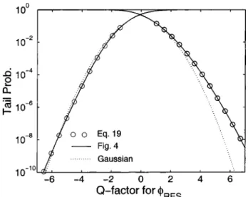
Figure 5 shows the cumulative tail probabilities as a function of the Q factor for RES, defined as Q⫽ (RES
⫺ RES)/RES, whereRESand RES
2 are the mean and
variance of the residual nonlinear phase noise shown in the appendix. The cumulative tail probabilities calcu-lated by numerical integration according to Eq. (19) is shown as circles, the model as the summation of a Gauss-ian random variable and the difference of two noncentral 2random variables with two degrees of freedom of Fig. 4
is shown as solid lines, and the Gaussian assumption1,6,7 is shown as dotted lines. From Figs. 1 and 4, the pdf of RESresembles a Gaussian pdf with mean and variance
from Ref. 8 and the appendix. The residual nonlinear phase noise of RES can be modeled accurately as a
Gaussian random variable, especially for the tail prob-abilities less than the mean. Even for the tail probabili-ties larger than the mean, the Gaussian model forRESis
better than that for NL. If the tail probabilities for
⬎10⫺5is of interest, Gaussian approximation for REScan
be used. Fig. 3. Cumulative tail probability ofNLas compared with the
model of Fig. 2 and a Gaussian approximation.
Fig. 4. pdf ofRESis the convolution of a Gaussian pdf and two noncentral2pdf ’s with two degrees of freedom.
Fig. 5. Cumulative tail probability ofRESas compared with the model of Fig. 4 and a Gaussian approximation.
4. CONCLUSION
The characteristic functions of nonlinear phase noise, with and without the correction using the received inten-sity, are derived analytically as a product of N noncentral 2 characteristic functions with two degrees of freedom.
The pdf ’s are calculated exactly as the inverse Fourier transform of the characteristic functions. The pdf of the nonlinear phase noise can be modeled as the convolution of a Gaussian pdf and a noncentral 2 pdf with two
de-grees of freedom. Using the received intensity to correct for the phase noise, the pdf of the residual nonlinear phase noise can be modeled accurately as the convolution of a Gaussian pdf and two noncentral2 pdf ’s with two
degrees of freedom. The Gaussian approximation of the residual nonlinear phase noise is much better than that for nonlinear phase noise.
APPENDIX A: OPTIMAL LINEAR
COMPENSATOR
This appendix shows important results from Ref. 8. The optimal scale factor to minimimize the variance ofRESis
␣opt⫽ N⫹ 1 2 A2⫹ 共2N ⫹ 1兲2/3 A2⫹ N2 ⬇ N⫹ 1 2 . (21) The variance of the residual nonlinear phase noise of Eq. (15) is reduced to
2RES⫽ 共N ⫺ 1兲N共N ⫹ 1兲2
⫻A
4⫹ 2N2A2⫹ 共2N2⫹ 1兲4/3
3共A2⫹ N2兲 (22)
from that of the nonlinear phase noise of
NL 2 ⫽ 4 3N共N ⫹ 1兲 2
冋冉
N⫹ 1 2冊
A 2 ⫹ 共N2⫹ N ⫹ 1兲2册
. (23)The mean of the nonlinear phase noise Eq. (1) is
NL⫽ N关A2⫹ 共N ⫹ 1兲2兴. (24)
The mean of the residual nonlinear phase noise is RES⫽NL⫺␣opt共A2⫹ 2N2兲. (25)
REFERENCES
1. J. P. Gordon and L. F. Mollenauer, ‘‘Phase noise in photonic communications systems using linear amplifiers,’’ Opt. Lett. 15, 1351–1353 (1990).
2. S. Ryu, ‘‘Signal linewidth broadening due to nonlinear Kerr effect in long-haul coherent systems using cascaded optical amplifiers,’’ J. Lightwave Technol. 10, 1450–1457 (1992). 3. A. H. Gnauck, G. Raybon, S. Chandrasekhar, J. Leuthold,
C. Doerr, L. Stulz, A. Agrawal, S. Banerjee, D. Grosz, S. Hunsche, A. Kung, A. Marhelyuk, D. Maymar, M. Movas-saghi, X. Liu, C. Xu, X. Wei, and D. M. Gill, ‘‘2.5 Tb/s (64 ⫻ 42.7 Gb/s) transmission over 40 ⫻ 100 km NZDSF us-ing RZ-DPSK format and all-Raman-amplified spans,’’ in Optical Fiber Communication Conference (Optical Society of America, Washington, D.C., 2002), postdeadline paper FC2.
4. R. A. Griffin, R. I. Johnstone, R. G. Walker, J. Hall, S. D. Wadsworth, K. Berry, A. C. Carter, M. J. Wale, P. A. Jerram, and N. J. Parsons, ‘‘10 Gb/s optical differential quadrature phase shift key (DQPSK) transmission using GaAs/AlGaAs integration,’’ in Optical Fiber Communication Conference (Optical Society of America, Washington, D.C., 2002), post-deadline paper FD6.
5. B. Zhu, L. Leng, A. H. Gnauck, M. O. Pedersen, D. Peck-ham, L. E. Nelson, S. Stulz, S. Kado, L. Gruner-Nielsen, R. L. Lingle, S. Knudsen, J. Leuthold, C. Doerr, S. Chan-drasekhar, G. Baynham, P. Gaarde, Y. Emori, and S. Namiki, ‘‘Transmission of 3.2 Tb/s (80⫻ 42.7 Gb/s) over 5200 km of UltraWave™ fiber with 100-km dispersion-managed spans using RZ-DPSK format,’’ presented of the 28th European Conference on Optical Communication, Copenhagen, Denmark, September 9–12, 2002, postdead-line paper PD4.2.
6. X. Liu, X. Wei, R. E. Slusher, and C. J. McKinstrie, ‘‘Improv-ing transmission performance in differential phase-shift-keyed systems by use of lumped nonlinear phase-shift com-pensation,’’ Opt. Lett. 27, 1616–1618 (2002).
7. C. Xu and X. Liu, ‘‘Postnonlinearity compensation with data-driven phase modulators in phase-shift keying trans-mission,’’ Opt. Lett. 27, 1619–1621 (2002).
8. K.-P. Ho and J. M. Kahn, ‘‘Detection technique to mitigate Kerr effect phase noise,’’ http://arXiv.org/physics/0211097. 9. G. L. Turin, ‘‘The characteristic function of Hermitian
qua-dratic forms in complex normal variables,’’ Biometrika 47, 199–201 (1960).
10. J. G. Proakis, Digital Communications, 4th ed. (McGraw-Hill, New York, 2000).
11. R. M. Gray, ‘‘On the asymptotic eigenvalue distribution of Toeplitz matrices,’’ IEEE Trans. Inf. Theory IT-18, 725–730 (1972).