MAVTgsa: An R Package for Gene Set (Enrichment) Analysis

MAVTgsa: an R package for gene set (enrichment)

analysis

Chih-Yi Chien

_{, Ching-Wei Chang}

_{, Chen-An Tsai}

_{, and James J.}

Chen

1 _{Community Medicine Research Center, Keelung Chang Gung Memorial Hospital, No. 200, Lane 208,} Jijinyi Rd, Anle District, Keelung, 204, Taiwan.

2 _{Division of Bioinformatics and Biostatistics, National Center for Toxicological Research, FDA, 3900} NCTR Road, Jefferson, AR 72079.

3 _{Department of Agronomy, National Taiwan University, No. 1, section 4, Roosevelt Road, Taipei 106,} Taiwan.

4 _{Graduate Institute of Biostatistics and Biostatistics Center, China Medical University, Taichung, Taiwan}

E-mails:

Chih-Yi Chien 92354503@nccu.edu.tw Chen-An Tsai catsai@ntu.edu.tw

Ching-Wei Chang ching-wei.chang@fda.hhs.gov James J. Chen jamesj.chen@fda.hhs.gov

*Correspondence: Dr. James J. Chen 3900 NCTR Road, HFT-20 Jefferson, AR 72079, USA TEL: (870) 543-7007 FAX: (870) 543-7662 Email: jamesj.chen@fda.hhs.gov Prof. Chen-An Tsai

Department of Agronomy National Taiwan University No. 1, section 4

Roosevelt Road, Taipei 106, Taiwan.

Email: catsai@ntu.edu.tw

+ _{These authors contributed equally to this work.}

The views presented in this paper are those of the authors and do not necessarily represent those of the U.S. Food and Drug Administration

Abstract

Gene-set analysis methods aim to determine whether an a priori defined set of genes shows statistically significant difference in expression on either categorical or continuous outcomes. . Although many methods for gene set analysis have been proposed, a systematic analysis tool for identification of different types of gene set significance modules has not been developed previously. This work presents an R package, called MAVTgsa, which include three different methods for integrated gene set enrichment analysis. 1) The one-sided OLS (ordinary least squares) test detects coordinated changes of genes in gene set in one direction, either up- or down-regulation. 2) The two-sided MANOVA (multivariate analysis variance) detects changes both up- and down-regulation for studying two or more experimental conditions. 3) A Random Forests-based procedure is to identify gene sets that can accurately predict samples from different experimental conditions or are associated with the continuous phenotypes. MAVTgsa computes the p-values and FDR (false discovery rate) q-values for all gene sets in the study. Furthermore,

MAVTgsa provides several visualization outputs to support and interpret the enrichment results. This package is available online at http://cran.r-project.org/web/packages/MAVTgsa/

1 Introduction

DNA microarray technology enables simultaneous monitoring of the expression level of a large number of genes for a given experimental study. Much initial research on methods for data analysis has focused on the techniques to identify a list of differentially expressed genes. After selection of a list of differentially expressed gene, the list is then examined with biologically predefined gene sets to determine whether any sets are overrepresented in the list compared with the whole list ([1-3]). Mootha et al. [4] proposed Gene Set Enrichment Analysis (GSEA), which considers the entire distribution of a predefined gene set rather than a subset from the differential expression list. GSEA provides a direct approach to the analysis of gene sets of interest and the results are relatively easy to interpret. Furthermore, microarray experiments inherit various sources of biological and technical variability, and analysis of a gene set is expected to be more reproducible than an individual gene analysis.

GSEA is a statistical approach to determine whether a functionally related set of genes expresses differently (enrichment and/or deletion) under different experimental conditions. The GSEA approach has inspired the development of various statistical tests for identifying differentially expressed gene sets [5-16]. There are two fundamental hypotheses for GSEA: competitive hypothesis and self-contained hypothesis [8]. The competitive hypothesis tests if the association of a gene set with the phenotype is equal to those of the other gene sets. The self-contained hypothesis tests if the expression of a gene set differs by the experimental condition. In either test, re-sampling methods are typically used to generate the null distribution of test statistics. The null distributions of statistic under the competitive hypothesis are generated by gene sampling; the null distributions under the self-contained hypothesis are generated by subject-sampling. Various GSEA statistics have been proposed for testing either the competitive hypothesis or self-contained hypothesis. There are also hybrid-type methods that utilize gene and sample sampling (e.g., [5, 9]). The differences of the two hypotheses were evaluated and summarized in Nam and Kim [14] and Dinu et al. [15]. Gene sampling under the competitive hypothesis simply reassigns the genes into different gene sets. As a result, the sampled distributions are not independent. On the other hand, subject sampling is consistent with the null hypothesis, which the null distributions of statistical tests are identically and independently distributed. In addition, the self-contained hypothesis is a generalization

from identification of differentially expressed genes to identification of differentially expressed gene sets. Therefore, we consider self-contained hypothesis and corresponding permutation p-values in this paper. In this paper, a statistical test to determine whether some functionally predefined classes of genes express differently under different experimental conditions is referred to as gene set analysis (GSA). When there are two experimental conditions, a GSA can be a one-sided or two-sided test. A one-sided test is to detect the changes of gene expressions in the gene set in one direction, either up- or down-regulation. The two-sided test is to detect the changes in both up- and down-regulation [6, 15]. When the goal is to detect coordinated changes in one direction, the one-sided hypothesis is appropriate. However, in an exploratory context, it is impossible to pre-specify how individual genes in a gene set will respond in different conditions. Hence, two-sided hypothesis is generally suggested.

The original GSEA statistic was developed for a one-sided test to identify down-regulated genes in Type 2 diabetes mellitus subjects [4]. Other one-sided tests included: T-like statistic [8]; MaxMean statistic [9]; standardized weighted sum statistic [10] and OLS statistics [6]. Chen et al. [6] showed OLS statistic performed well for GSA statistics in one-sided test. Two-sided tests were considered in most GSA statistics (e.g., [7,11-17]). Tsai and Chen [16] proposed a multivariate analysis of variance (MANOVA) GSA test for two or more conditions. The MANOVA approach was compared with principal component analysis [13], SAM-GS [15], GSEA [5], MaxMean [9], analysis of covariance [7] and Goeman’s global test [11]. They found that MANOVA test performed the best in terms of control of type I error and power.

The GSEA software only performs one-sided test in two conditions at time [4]. Other software provides either one-sided or two-sided test; for example, BRB-Array tools [18] provided LS (KS) statistics, Goeman’s global test and MaxMean test. When the null hypothesis is that no genes in the gene set are differentially expressed, the two-sided is more appropriate than other methods.

When the purpose of study is to build up prediction rule based on gene expression profile, utilizing the existing biological knowledge, such as biological pathway or cellular function information, has been showed to improve the classification accuracy (e.g., [19-21]). The selection of predictors can be either preselected by testing or chosen based on classification algorithm, and the final identified predictors are also considered as differential expressed. Hsueh et al. [22] and Pang et al. [23] proposed a random

forests-based differential analysis of gene set data in terms of predictive performance of gene sets. The analysis contained not only a classifier but also the feature importance of the input gene sets.

The gene set analysis has been considered to accommodate continuous phenotype. Linear Combination Test [17] has been extended from binary to continuous phenotype (LCT) by utilizing linear regression function [24]. Significance Analysis of Microarrays for Gene Sets (SAM-GS) [15] and Global Test [11] have also been extended in a generalized linear model (GLM) framework. Dinu et al. [24] compared the type I error rates and powers for the three methods and concluded that LCT approach is powerful and computationally attractive. The random forests-based approach could be also applied to continuous phenotype by modifying random forest classification to random forest regression. A small simulation experiment to compare the random forests-based and LCT is reported in this paper.

The main purpose of this paper is to present the MAVTgsa R package tool for GSA for study with categorical phenotypes or continuous phenotypes. The OLS one-sided test, MANOVA test, and Random forest-based analysis are implemented in MAVTgsa. When categorical phenotypes involve more than two classes, the three multiple comparison procedures are implemented: Dunnett, Tukey, and sequential pairwise comparison. The program provides two visualization plots: GSA plot, a p-value plot of GSA for all gene sets in the study and GST, a plot of the empirical distribution function of the ranked test statistics of a selected gene set. The researcher is able to summarize and visualize the gene expression data in gene set analysis. More importantly, the adjusted p-value of family-wise error rate (FWER) [25] and FDR step-up procedure [26] are computed in this package. When the outcome of interest is a continuous phenotype, the random-forests based analysis is applied in the regression context. Figure 1 describes the procedure how to implement the MAVTgsa package for gene-set enrichment analysis.

The following second section describes the methods implemented in the MAVTgsa package. In the third section, we present a description of the MAVTgsa package including data input, optional parameters, output and result visualization. In the fourth section, we apply to two real data sets, P53 and breast cancer, for illustration. This paper is concluded by a summary.

2 Methods

The OLS test was developed to detect changes in one direction, either up- or down-regulation, for a study with two experimental conditions. Consider a gene set consisting of m genes with two conditions of sample size n1 and n2. Let yij = (yij1,…, yijm) be the m-vector of intensities for simple j (j = 1,…, ni) in i-th

condition (i = 1,2). Denote the standardized variable y*

ijk = (yijk –y )/sk k, where y is the overall sample k mean for the k-th gene and sk is the pooled standard deviation. Let zik = Σj y*ijk/ni be the mean of the

standardized variable for the k-th in the i-th condition. Denote the zi = (zi1,…, zim) as the m-vector of the standardized mean variable zij’s for the i-th condition (i = 1, 2). Let di be an m-dimensional vector for the

mean difference between two conditions di = (z1 - z2). The O'Brien's OLS statistic [27] is

_

_

T

1

1

1'

V

d

'



where 1 is a mi × 1 vector of 1's and Vi is the pooled sample covariance matrix of di. If di is a multivariate

normal, then the OLS statistic Tols has an approximately t distribution with n1 + n2 – 2 degrees of freedom.

The one-sided OLS statistic is the most widely used global test for the analysis of multiple clinical endpoints [27]. This test is very powerful when the changes in the gene expression are in the same direction. The direction of changes of significant gene set can be checked from the OLS statistic The OLS statistics account for gene set size and correlation structure [6]. In addition, the permutation p-values for the OLS test are suggested to compute as the level of significance.

2.2 The MANOVA test

Consider a gene set consisting of m genes with c conditions of sample size n1,…, nc. Let yij = (yij1,… yijm) be the m-vector of intensities for simple j (j = 1,…,ni) in i-th condition (i = 1,…,c). The MANOVA model [16] can be expressed as yij = i + eij, where eij is vector of residuals with Var(eij) = and i is the m-vector of means for the i-th condition. MAVTgsa occupied the Wilks’  as the statistic for MANOVA test. The formula of Wilks’  is given as

Where ks are the eigenvalues of the matrix S (= E-1_{H), and E is within sum of squares matrix (sample} covariance matrix) and H is between sum of squares matrix. The number of eigenvalues k is equal to the minimum of the number of genes (m) and the number of conditions minus 1 (c-1). When the number of genes in the gene set is grater than the number of samples, the matrix E is singular and ill-condition. The shrinkage covariance matrix estimator (Sij*_{) proposed by Schafer and Strimmer [28] is applied to estimate} the sample covariance matrix and given as

      if if * * j i s s r j i s s jj ii ij ii ij

and * _ min{1,max(0,1_ˆ*)}

ij ij r

r , where s and ii r respectively denote the empirical sample ij

variance and sample correlation, and the optimal shrinkage intensity

_







The distribution of Wilks’ under the null hypothesis of no difference in responses among the conditions was estimated by the permutation method. The Wilks’s test is equivalent to Hotelling’s T2 _{test when} there are only two conditions. The Hotelling’s T2 _{statistic is}

(

)

(

)

_x

_x

_S

_x

_x

n

n

n

n

T

_







where x and i S denote the sample mean vector and sample covariance matrix of the i-th group (i = i

1,2), respectively, and Sp ((n11)S1 (n21)S2)/(n1n2 2)denotes the pooled covariance matrix. Using the shrinkage covariance matrix and permutation test, the p-values of the Hotelling’s T2 _test are computed. The p-values of the MANOVA test are computed using the permutation method.

The MANOVA test is a multivariate generalization of the univariate analysis of variance (ANOVA) as the Hotelling’s T2 _{test is the generalization of the univariate t-test. The parametric MANOVA and T}2 _test statistics are commonly used for analyzing multivariate data. The MANOVA test uses a shrinkage covariance matrix estimator [28] to incorporate the correlations structure among the genes in the test statistic and account for the singularity and ill-condition of the sample covariance matrix. The MANOVA test uses the permutation method to compute the p-values. Tsai and Chen [16] have compared the

MANOVA test with several GSEA tests including the two one-sided tests: GSEA [5] and MaxMean [9], and four two-sided tests: ANCOVA [7], Global [11], PCA [13], and SAM-GS [15]. Their simulation showed that MANOVA test perform well in terms of controlling the Type I error and power as compared to other tests, except that the ANCOVA [7] was more powerful when the variances were equal across all genes in the gene set.

2.3 Random-forests based analysis

The Random Forests (RF) [29] is a popular classification and regression algorithm based on an ensemble of many classification/regression trees combined with a bootstrap sample out of the original dataset. The error rate of a classification tree or the mean of squared error (MSE) of a regression tree is calculated by the

observations outside the bootstrap sample called the out-of-bag (OOB) data. Lower error rate and MSE indicates that the corresponding gene set is with higher

prediction accuracy for a categorical phenotype and higher percent variance explained for a continuous phenotype, respectively. The variable selection for each split at the nodes of trees is conducted only from a small random subset of the predictors, so that there is no need to deal with the “small n large p” problem. A permutation based P-value can be obtained as





,

N

R

R

I

value

P









where R is the observed score from the Random Forests analysis, 0

R

permutation, and N is the total number of permutations. The score is calculated as the OOB error rate and MSE for the categorical and continuous phenotypes, respectively. The gene set is considered as

significantly expressed if the correspondent p-value is less than or equal to the significance level α. To measure the importance of each predictor variable, the Random Forests algorithm assesses the importance of a variable by looking at how much prediction error increases or MSE decreases when that variable of the (OOB) data is permuted while remaining variables are left unchanged. Here, the mean decrease in the

Gini index (MDG) and the mean decrease in MSE are employed as the importance measures of genes for categorical and continuous phenotypes, respectively.

2.4 Multiple comparisons methods

In MANOVA test, the null hypothesis is rejected if one or more of the mean differences or some combination of mean differences among the genes in gene set differs from zero. If the null hypothesis is rejected, three multiple comparison procedures are implemented to identify which two conditions differ in expression between gene sets for studies with more than two conditions. Three multiple comparisons methods are Dunnett, Tukey, and sequential pairwise comparison. Dunnett test is specifically designed for situations where all groups are to be compared against the "reference" group. Tukey test is for all pairwise comparisons. When the conditions are in order, sequential pairwise comparison is appropriate to be occupied for comparing with previous condition.

3 MAVTGSA package description

MAVTgsa is a software tool to evaluate the expressions of a priori defined gene sets under different experimental conditions. The package implements essentially the method described in the previous section and the main functions are MAVTn() and MAVTp().

3.1 MAVTn

For experiments with two or more than two conditions, the input parameters to perform the testing are described as follows.

MAVTn(DATA, GS, alpha, nbPerm, MCP)

 DATA is a gene expression data matrix with samples in columns. The first row contains the information of the experimental condition of each sample. The remaining rows contain gene expression.

 GS is a binary matrix coded 0 or 1 with genes in rows. Each column represents a pre-defined gene set, with row equal to 1 indicating that the gene is in the gene set, and 0 otherwise.

 nbPerm specifies the number of permutations, and at least 5,000 is recommended.

 MCP specifies one of three multiple comparison methods, Dunnett = 1, Tukey = 2, Sequential pairwise comparison = 3. MCP can be ignored when the number of experimental conditions is 2. The output of the MAVTn() function is a list of objects which contains:

 p value: a list of the gene sizes and the p-values and adjusted p-values of the statistical tests for GSA. The adjusted p-values of the family-wise error rate (FWE) [25] and the FDR step-up procedure [26] are computed using permutation method. In case of two experimental conditions, the p-values and adjusted p-values for OLS and Hotelling’s T2 _{test are listed. In case of more than two conditions, the} p-values for MANOVA and post hoc tests are listed.

 significant gene set: a list of the p-values of individual genes for those significant gene sets in statistical test of GSA.

In addition, a plot of p-values for all gene sets is drawn to examine the adequacy of the assumptions on which the distributions of the test statistics are based.

Example of applying MAVTn to a simulated 3 conditions data is as follows:

R> mu <- c(rep(1,5),rep(5,5)) R> Sigma <- diag(1,10)

R> set.seed(10) # fix random seed

R> GE <- rmvnorm(15,mu,Sigma) # generate 15 samples with 10 gene expression R> set.seed(10) # fix random seed

R> GS <- matrix(1*(runif(40,0,1)<=0.7),ncol=4,nrow=10) # simulate gene set matrix R> cl <- c(rep(1,5),rep(2,5),rep(3,5)) #clinical treatment

R> data <- rbind(cl,t(GE)) R> MAVTn(data,GS,MCP=1)

3.2 MAVTp

For experiments with categorical or continuous phenotypes, the input parameters to perform the Random Forests analysis are described as follows.

 DATA is a gene expression data matrix with samples in columns. The first row contains the

information of the experimental condition of each sample. The remaining rows contain gene expression.If a factor, classification is assumed, otherwise regression is assumed.

 GS could be a binary matrix coded 0 or 1 with genes in rows. Each column represents a pre-defined gene set, with row equal to 1 indicating that the gene is in the gene set, and 0 otherwise.

 nbPerm specifies the number of permutations.  Numoftree specifies the number of trees to grow.  Type indicates categorical or continuous phenotype.  Impt is an option for outputting the important measure.

The output of the MAVTp() function is a list of objects which contains:  p value: a list of the p-values of the random forests for GSA.

 important gene set: a list of the importance measurement of individual genes for those significant gene sets.

Example of applying MAVTp to a simulated continuous phenotype data is as follows:

R> mu <- c(rep(1,5),rep(5,5)) R> Sigma <- diag(1,10)

R> set.seed(15) # fix random seed

R> GE <- rmvnorm(15,mu,Sigma) # generate 15 samples with 10 gene expression R> y=mvrnorm(1,rep(0,10),diag(rep(1,10))) # generate continuous phenotype R> data <- rbind(y,GE)

R> GS <- matrix(1*(runif(30,0,1)<=0.7),ncol=3,nrow=10) # simulate gene set matrix R> test_rf_con <- MAVTp(data,GS,nbPerm=1000, numoftree=500,type="cont",impt=TRUE)

3.3 Visualization plots

Two visualization plots are implemented, GSA and GST. The GSA plot (Figure 2) provides a p-value plot of all gene sets considered in the study. The p-value plot is the plot of ordered p-value vs. its rank. The P-value plot can provide an overall assessment of differences in expression among conditions for all gene sets considered in the study. Under the null hypothesis of no differences, the P-values should be uniformly

distributed on the interval (0, 1); the P-value plot should be a straight line. If a null hypothesis is not true, then its P-value will tend to be small. The GST plot displays the relative direction (in two conditions) and statistics ranking for genes in a gene set. The GST plot is derived from the SAFE plot which provides the empirical distribution function for the ranked statistics of a given gene category [30]. The GST plot displays the ranked test statistics (red line) and empirical cumulative distribution function of these test statistics for expressed genes in a gene set (solid line). Tick marks above the plot display the location of genes with gene names. The shaded regions are set to represent the statistics that the p-values below the given alpha value (Figs 3-5 below). The input parameters to perform the analysis are described as follows. Two examples are presented in next section to show the output of GST plot.

4 Results

4.1 P53 study

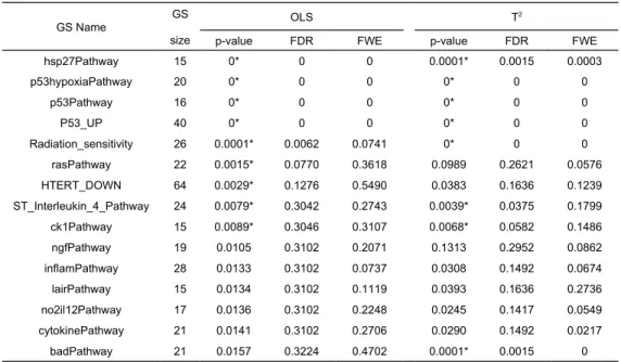
The MAVTgsa was applied to a P53 dataset. The p53 dataset is from a study to identify targets of the transcription factor p53 from 10,100 gene expression profiles in the NCI-60 collection of cancer cell lines. There are 308 gene sets in the p53 study. The mutation status of the p53 gene has been reported for 50 cell lines included 17 wild-type and 33 mutation samples. The dataset is publicly available at the GSEA website (http://www.broad.mit.edu/gsea). Table 1 shows the result of fifteen gene sets in which the p-values for OLS test are the top fifteen smallest p-p-values under 10,000 permutations (nbPerm=10,000). The significant level is set as 0.01 (alpha=0.01). The p-values for OLS test and MANOVA (Hotelling’s T2₎ were calculated and listed the p-values of individual genes for those significant gene sets. The p-values from the OLS test are different from the p-values from two-sided T2_{. The gene set rasPathway,}

HTERT_DOWN and ngfPathway are highly significant (p<0.01) by OLS test but they are not significant in Hotelling’s T2 _{test. In contrary, the gene set badPathway is highly significant in Hotelling’s T}2 _{test but} not in OLS test. Figure 2 is the GSA-plot for two groups. Figure 3 and 4 are the GST plots for the gene set rasPathway and badPathway respectively. In Figure 3, two of 22 genes are underexpressed with the p-value less than 0.01. On the other hand, one of 21 genes in badPathway shows underexpressed and one shows overexpressed in Figure 4. The results indicate that the power of methods to detect differential expressed gene set depends on the global pattern of genes within gene set. Combining the information

from the two tests and GSA-plot will be useful to get biological meaningful interpretation. The complete list of all p-values of gene sets and of individual genes for significant gene sets are available as

supplementary materials.

4.2 Breast cancer dataset

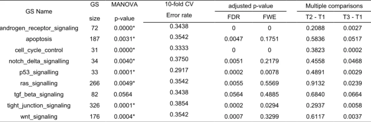
We applied the MAVTgsa to a breast cancer dataset [31] and illustrate the RF, MANOVA, and a multiple comparison analysis. The dataset consisted of three conditions with 1,113 genes and 96 samples. Three conditions were tumor grades 1, 2, and 3 with the sample sizes of 11, 25 and 60, respectively. There were nine cancer related pathways for gene set analysis. Table 2 shows the p-values of the MANOVA and the post-hoc Dunnett’s analysis for each of the nine pathways. Figure 5 is the GST plots for the 31 genes in the gene set cell_cycle_control. Five of the 31 genes are differential expressed with p-value less than 0.01 in the breast cancer samples. In this analysis the total computation time used to perform the analysis was approximately four hours and 10 minutes with nbPerm = 10,000. Two supplementary files contain the output of the analysis of this data set and P-53 study. A classification rule to classify the three tumor grades is also constructed. The error rates of 10-fold cross validation are given in Table 2.

4.3 Simulation study

In order to understand how well the random-forests based analysis performs for continuous phenotypes, we conducted a number of simulations to evaluate the performance in terms of type I error and power and compare to the LCT method [24]. The simulation design was similar to that considered by Dinu et al. [24]. For each gene set of size p, 24we generated a p by n gene expression matrix Xn×p with sample size of n and

a linear model was used to simulate the phenotype data associated with the gene set X. The gene

expressions matrix X was generated from a multivariate normal distribution with mean from a uniform (0, 10) distribution, variance from a uniform (1, 5) distribution, and a mixed intra-gene set correlation structure as follows

























;

,

0

;

2

1

,

;

1

,

otherwise

p

j

i

p

p

j

i







where the correlation ρ was set at 0, 0.3, 0.5 and 0.9 in this study. For each gene set, a continuous phenotype vector Yn×1 is generated from a multivariate normal distribution MVN(Xμ, I), where μ is the

effect size vector with length p and I the identity covariance matrix. In the null model, with no association of gene expressions on the phenotype, we set μ to be 0 to investigate the type I error and the simulation scenarios varied according to: sample sizes (n = 10, 20 or 50), gene set sizes (p = 20, 100 or 200) and the levels of correlation among genes (ρ=0, 0.3, 0.5 or 0.9) within a gene set at different number of genes (p1=5, 20 or 40). In the alternative model, the sample size and gene set size were respectively fixed at 20 and 100, as well as only 10 of genes were simulated to be associated with the phenotype to investigate power of two gene set analysis methods. First, we randomly generated 5 of the first 20 components of μ from normal distribution N(ν, |ν|) and another five of the next 20 components of μ from normal

distribution N(-ν, |ν|) as up- and down-regulated genes, respectively. The rest of components of μ were set to be 0. The effect sizes (ν) for the associations were set at 0.2, 0.6, 1.0, 1.4 and 1.8. For each scenario, the simulation data were replicated 1000 times to estimate type I error rate or power. The p-values were based on 1000 permutations. Power was then estimated as the proportion of significance using the nominal level of 0.05. Table 3 showed the empirical type I errors using the nominal level of 0.05 for each scenario. The type I errors from the Random Forests method were reasonably close to or below the nominal level, while the LCT method appeared to have an inflated type I error rate in most cases. It indicates that the RF method gives a conservative conclusion. Such conservativeness may lead to power loss in detecting a difference. Figure 6 illustrated the empirical powers using the nominal level of 0.05 for ρ = 0.0, 0.3, 0.6 and 0.9. As expected, the RF method was slightly inferior to the LCT method, while LCT was unable to adequately control the type I error rate. However, with increasing of correlations among genes, both methods appeared to be equivalent. The powers of both methods increased gradually with increasing correlations.

In addition, to explore the robustness of the RF method with regard to non-linear association data, the continuous phenotype vector Yn×1 was generated from a multivariate normal distribution MVN(exp(Xμ), I). Figure 7 showed the average power over 1000 simulations for each method using the nominal level of

0.05. As a result, the RF provided a more powerful test than the LCT method to detect the non-linear association between gene sets and continuous phenotypes.

5 Conclusion

The MAVTgsa package performs a systematic gene set analysis for identification of different types of gene-set significance modules. The user can select the most appropriate analysis or combine them to provide insight into gene sets that respond in a similar manner to varying phenotypes and that might therefore be co-regulated. For studies with more than two conditions, MAVTgsa not only provides the MANOVA test to identify gene sets consisting of differentially expressed genes but also implements three multiple comparison methods for post-hoc analysis. The method implemented in MAVTgsa package has the advantage of real application. First, the MAVTgsa package provides the adjusted p-values using both family-wise error rate (FWER) [25] and the FDR step-up procedure [26] using permutation method. Second, MAVTgsa is a permutation-based method to compute p-values and adjusted p-values. Third, MAVTgsa displays the results for individual genes test of significant gene sets. Finally, MAVTgsa draws the GST plot to display the empirical cumulative function for the ranked test statistics of a given gene set with the gene location and gene name above the plot. These allow the user to analyze the interesting gene set of the data easily. In addition, MAVTgsa provides a Random Forests-based procedure to identify gene sets in terms of predictive performance or in association with the continuous phenotypes. Random forests method has been proved to perform well in comparison with the other classification methods and

successfully applied to various problems. Most importantly, it can accommodate multi-class and continuous phenotypes for the GSA, even if the associations between gene sets and phenotypes are nonlinear and involve complex high-order interaction effects.

6 HARD WARE AND SOFTWARE SPECIFICATIONS

The implementation and examples run of this package was conducted on a laptop computer with 2.8 GHz CPU and 3.0GB RAM under the Microsoft Windows XP Professional SP3 using the R software version 2.14.1.

The MAVTgsa package is available from http://cran.r-project.org/web/packages/MAVTgsa/.

8 COMPETING INTERESTS

The authors declare that they have not competing interests.

9 ACKNOWLEDGEMENTS

Chih-Yi’s research was supported by the Post-doctoral Fellowship Program at the NCTR administered by the Oak Ridge Institute for Science and Education through an interagency agreement between USDOE and USFDA. The views presented in this paper are those of the authors and do not necessarily represent those of the U.S. Food and Drug Administration.

References

[1] S. Draghici, S.A. Krawetz, Global functional profiling of gene expression, Genomics 81 (2003) 98– 104.

[2] P. Khatri, S. Draghici, Ontological analysis of gene expression data: current tools, limitations, and open problems, Bioinformatics 21 (2005) 3587–3595.

[3] I. Rivals, L. Personnaz, L. Taing, M.C. Potier, Enrichment or depletion of a GO category within a class of genes: which test? Bioinformatics 23 (2007) 401–407.

[4] V.K. Mootha, C.M. Lindgren, K.F. Eriksson, A. Subramanian, S. Sihag, J. Lehar, P. Puigserver, E. Carlsson, M. Ridderstråle, E. Laurila, N. Houstis, M.J. Daly, N. Patterson, J.P. Mesirov, T.R. Golub, P. Tamayo, B. Spiegelman, E.S. Lander, J.N. Hirschhorn, D. Altshuler, L.C. Groop, PGC-1 alpha-responsive genes involved in oxidative phosphorylation are coordinately downregulated in human diabetes, Nat. Genet. 34 (2003) 267–273.

[5] A. Subramanian, P. Tamayo, V.K. Mootha, S. Mukherjee, B.L. Ebert, M.A. Gillette, A. Paulovich, S.L. Pomeroy, T.R. Golub, E.S. Lander, J.P. Mesirov, Gene set enrichment analysis: A knowledge-based approach for interpreting genome-wide expression profiles, Proc. Natl. Acad. Sci. 102 (2005) 15545–15550.

[6] J.J. Chen, T. Lee, R.R. Delongchamp, T. Chen, C.A. Tsai, Significance analysis of groups of genes in expression profiling studies, Bioinformatics 23 (2007) 2104–2112.

[7] U. Mansmann, R. Meister, Testing differential gene expression in functional groups: Goeman’s global test versus an ANCOVA approach, Method. Inform. in Med. 44 (2005) 449–453.

[8] L. Tian, S.A. Greenberg, S.W. Kong, J. Altschuler, I.S. Kohane, P.J. Park, Discovering statistically significant pathways in expression profiling studies, Proc. Natl Acad. of Sci. 102 (2005) 13544–13549. [9] B. Efron, R. Tibshirani, On testing the significance of sets of genes, Ann. Appl. Statist. 1 (2007) 107–

129.

[10] J. Läuter, Exact t and F tests for analyzing studies with multiple endpoin ts, Biometrics 52 (1996) 964–970.

[11] J.J. Goeman, S.A. van de Geer, F. de Kort, H. C. van Houwelingen, A global test for groups of genes: testing association with a clinical outcome, Bioinformatics 20 (2004) 93–99.

[12] J. Tomfohr, J. Lu, T.B. Kepler, Pathway level analysis of gene expression using singular value decomposition, BMC Bioinformatics 6 (2005) 225.

[13] S.W. Kong, W.T. Pu, P.J. Park, A multivariate approach for integrating genome wide expression data and biological knowledge, Bioinformatics 22 (2006) 2373–2380.

[14] D. Nam, S.Y. Kim, Gene-set approach for expression pattern analysis. Brief Bioinform, 9 (2008) 189-197.

[15] I. Dinu, J.D. Potter, T. Mueller, Q. Liu, A.J. Adewale, G.S. Jhangri, G. Einecke, K.S. Famulski, P. Halloran, Y. Yasui, Improving gene set analysis of microarray data by SAM-GS, BMC Bioinformatics 8 (2007) 242.

[16] C.A. Tsai, J.J. Chen, Multivariate analysis of variance test for gene set analysis, Bioinformatics 25 (2009) 897–903.

[17] X. Wang, I. Dinu, W. Liu, Y. Yasui, Linear combination test for hierarchical gene Set analysis. Stat Appl Genet Mol Biol 10 (2011) Article 13.

[18] Simon, R. BRB-Array tools version 4.3 user’s manual. Biometrics Research Branch. National Cancer Institute. 2012. http://linus.nci.nih.gov/BRB-ArrayTools.html

[19] J. Kang J, A.D. D'Andrea AD, D. Kozono, A DNA repair pathway-focused score for prediction of outcomes in ovarian cancer treated with platinum-based chemotherapy. J Natl Cancer Inst 104 (2012) 670-681.

[20]T.P. Lu, L.C. Lai, M.H. Tsai MH et al., Integrated analyses of copy number variations and gene expression in lung adenocarcinoma. PLoS One 6 (2011) e24829.

[21]E. Bicaku, Y. Xiong, D.C. Marchion et al., In vitro analysis of ovarian cancer response to cisplatin, carboplatin, and paclitaxel identifies common pathways that are also associated with overall patient survival. Br J Cancer 106 (2012) 1967-1975.

[22]H.M. Hsueh, D.W. Zhou, C.A. Tsai, Random forests-based differential analysis of gene sets for gene expression data. Gene 518 (2013) 179-186.

[23]H. Pang, A. Lin, M. Holford, B. Enerson, B. Lu, M. Lawton, E. Floyd, H. Zhao, Pathway analysis using random forests classification and regression. Bioinformatics 22 (2006) 2028-2036.

[24] I. Dinu, X. Wang, L.E. Kelemen, S. Vatanpour, S. Pyne, Linear combination test for gene set analysis of a continuous phenotype, BMC Bioinformatics 14 (2013) 212.

[25] P.H. Westfall, S.S. Young, Resampling-based multiple testing: Examples and methods for p-value adjustment. (John Wiley & Sons, New York US, 1993).

[26] Y. Benjamini, Y. Hochberg, Controlling the false discovery rate: a practical and powerful approach to multiple testing. J. R. Stat. Soc. Ser. B 57 (1995) 289–300.

[27] P.C. O'Brien, Procedure for comparing samples with multiple endpoints, Biometrics 40 (1984) 1079– 1087.

[28] J. Schäfer, K. Strimmer, A shrinkage approach to large-scale covariance matrix estimation and implications for functional genomics. Statist. Appl, Genet. Mol. Biol. 4 (2005) 32.

[29] L. Breiman, Random forest. Mach Learn .45 (2001) 5-32.

[30] W.T. Barry, A.B. Nobel, F.A. Wright, Significance analysis of functional categories in gene expression studies: a structured permutation approach. Bioinformatics 21 (2004) 1943-1949.

[31] L.J. van't Veer, H. Dai, M.J. van de Vijver, Y.D. He, A.A.M. Hart, M. Mao, H.L. Peterse, K. van der Kooy, M.J. Marton, A.T. Witteveen, G.J. Schreiber, R.M. Kerkhoven, C. Roberts, P.S. Linsley, R. Bernards, S.H. Friend, Gene expression profiling predicts clinical outcome of breast cancer, Nature 415 (2002) 530-536.

Table 1. The original p-values and adjusted p-values (FDR and FWE) of the OLS and Hotelling’s T2 _{test of P53 data.}

GS Name GS

size

OLS T2

p-value FDR FWE p-value FDR FWE

hsp27Pathway 15 0* 0 0 0.0001* 0.0015 0.0003 p53hypoxiaPathway 20 0* 0 0 0* 0 0 p53Pathway 16 0* 0 0 0* 0 0 P53_UP 40 0* 0 0 0* 0 0 Radiation_sensitivity 26 0.0001* 0.0062 0.0741 0* 0 0 rasPathway 22 0.0015* 0.0770 0.3618 0.0989 0.2621 0.0576 HTERT_DOWN 64 0.0029* 0.1276 0.5490 0.0383 0.1636 0.1239 ST_Interleukin_4_Pathway 24 0.0079* 0.3042 0.2743 0.0039* 0.0375 0.1799 ck1Pathway 15 0.0089* 0.3046 0.3107 0.0068* 0.0582 0.1486 ngfPathway 19 0.0105 0.3102 0.2071 0.1313 0.2952 0.0862 inflamPathway 28 0.0133 0.3102 0.0737 0.0308 0.1492 0.0674 lairPathway 15 0.0134 0.3102 0.1119 0.0393 0.1636 0.2736 no2il12Pathway 17 0.0136 0.3102 0.2248 0.0245 0.1417 0.0549 cytokinePathway 21 0.0141 0.3102 0.2706 0.0290 0.1492 0.0217 badPathway 21 0.0157 0.3224 0.4702 0.0001* 0.0015 0 * Denote p-values < 0.01.

Table 2. Results of the MANOVA, 10-fold CV error and post-hoc test (Dunnett’s method) of breast cancer data with three groups for

GS Name GS size

MANOVA p-value

10-fold CV _{adjusted p-value Multiple comparisons}

Error rate _{FDR FWE T2 - T1 T3 - T1}

androgen_receptor_signaling 72 0.0000* 0.3438 0 0 0.2088 0.0027 apoptosis 187 0.0031* 0.3542 0.0047 0.1751 0.5836 0.0517 cell_cycle_control 31 0.0000* 0.3333 0 0 0.3823 0.0002 notch_delta_signalling 34 0.0040* 0.3750 0.0051 0.2179 0.4558 0.0468 p53_signalling 33 0.0001* 0.2917 0.0002 0.0078 0.4891 0.0029 ras_signalling 266 0.0049* 0.3542 0.0055 0.5569 0.9132 0.0239 tgf_beta_signaling 82 0.0564 0.3438 0.0564 0.4885 0.6840 0.0664 tight_junction_signaling 326 0.0001* 0.3854 0.0002 0.0294 0.2937 0.0058 wnt_signaling 176 0.0004* 0.3542 0.0007 0.3299 0.6117 0.0037

* Denote p-values < 0.01 in Wilks’  test.

Table 3. Type I error rate comparisons of two GSA methods for continuous phenotype, RF and LCT, at a

significance level of 0.05. Method ρ=0.0 ρ=0.3 ρ=0.6 ρ=0.9 n=10, p=20, p1=5 RF 0.050 0.049 0.046 0.036 LCT 0.052 0.060 0.044 0.052 n=20, p=100, p1=20 RF 0.051 0.042 0.049 0.052

LCT 0.060 0.051 0.050 0.064

n=50, p=200, p1=40

RF 0.052 0.040 0.040 0.052

FIGURES

Figure 1. A schematic flowchart of GSEA using the MAVTgsa package.

Figure 2. The GSA-plot for OLS test and Hotelling’s T2 _{test in P53 study. Both p-values in OLS test}

(black line) and T2 _{test (red line) are not close to the diagonal dash line. That means both tests could}

identify several gene sets showed truly significant of the testing hypotheses.

Figure 3. GST-plot for the gene set rasPathway in P53 dataset. The solid line is the empirical

cumulative distribution function of the rank t-statistics for 10,100 genes in the array. The two tailed shaded regions represent the t-statistics that had the p-value less than 0.01. There are 22 tick marks above the plot which display the location of the p-value of the genes from the gene set. The gene set shows

underexpressed.

Figure 4. GST-plot for the gene set badPathway in P53 dataset. The solid line

is the empirical cumulative distribution function of the rank t-statistics for 10,100 genes in the array. The two tailed shaded regions represent the t-statistics that had the p-value less than 0.01. There are 21 tick marks above the plot which display the location of the p-value of the genes from the gene set. The gene set shows both under- and overexpressed.

Figure 5. GST-plot for the gene set cell_cycle_control in breast cancer dataset. The solid line is the empirical cumulative distribution function of the rank

F-statistics for 1,113 genes in the array. The shaded regions represent the F-statistics that had the p-value less than 0.01. There are 5 tick marks above the plot which display the location of the p-value of the genes from the gene set.

Figure 6. Power comparisons of two GSA methods for a linear association between gene sets and continuous phenotypes: Random Forests and LCT.

Figure 7. Power comparisons of two GSA methods for a non-linear association between gene sets and continuous phenotypes: Random Forests and LCT.

 P ow er 0.2 0.4 0.6 0.8 1.0 0.5 1.0 1.5 =0.6 0.5 1.0 1.5 =0.9 0.2 0.4 0.6 0.8 1.0 =0 =0.3 RF LCT Figure 6.

 P ow er 0.2 0.4 0.6 0.8 1.0 0.5 1.0 1.5 =0.6 0.5 1.0 1.5 =0.9 0.2 0.4 0.6 0.8 1.0 =0 =0.3 RF LCT Figure 7.

Supplementary file 1

Description: The output of P53 study. It displays the p-values and adjusted p-values for OLS test and

Hotelling’s T2 test of 308 gene sets. The p-values for individual genes test of significant gene sets are provided.

Supplementary file 2

Description: The output of breast cancer study. It displays the p-values and adjusted p-values for