適應性加權損失管制圖之研究 - 政大學術集成

全文

(1)國立政治大學統計學系碩士學位論文指導教授:楊素芬博士適應性加權損失管制圖之研究政治. 大. The Study立of Adaptive Weighted Loss. ‧ 國. 學. Control Charts for Dependent Process Steps. ‧. n. er. io. sit. y. Nat. al. Ch. engchi. i Un. v. 研究生：林亮妤撰中華民國九十九年六月.

(2) 謝辭回想起，兩年前剛成為碩一新鮮人的期待，到今天能與大家分享收成的喜悅與展望未來，能有這一切要感謝許多人對我的幫助與鼓勵。本論文能順利完成，首先要感謝我的指導老師楊素芬教授。老師辛苦的指導，不僅讓我在統計品管的知識與應用精進不少，更讓我對做事的態度磨練的更加積極與具有責任感。感謝我的口試委員曾勝滄教授與呂明哲教授，兩位老師對本論文仔細地審閱並提出許多精闢的見解及意見，使得本論文能更臻完善。感謝我的同學，特別是伊萱、宜臻與政憲，研究所的日子因為有你們的陪伴，讓我增添許多歡笑與色彩。. 立. 政治大. 最後，我要感謝愛我的家人，謝謝你們一直陪伴在我身旁，當我永遠的避風. ‧ 國. 學. 港。. ‧. 本研究承蒙行政院國家科學委員會，計畫編號. NSC. sit. y. Nat. 96-2118-M-004-001-MY2，NSC 98-2118-M-004-005-MY2 及國立政治大學服務創. io. n. al. er. 新頂尖研究中心(CSI)補助，謹此致謝。. Ch. engchi. i Un. v. 林亮妤. 謹致. 中華民國九十九年六月.

(3) ABSTRACT Recent research has shown that control charts with adaptive features detect process shifts faster than traditional Shewhart charts. In this article, we propose three kinds of adaptive weighted loss ( WL ) control charts, variable sampling intervals (VSI) WL control charts , variable sample sizes and sampling intervals (VSSI) WL control charts and variable parameters (VP) WL control charts, to monitor the target and variance on a single process step and two dependent process steps simultaneously. These adaptive WL control charts may effectively distinguish which process step is out-of-control. We use the Markov chain approach to calculate the adjusted average. 治政 time to signal (AATS) and average number of observations 大 to signal (ANOS) in order 立 to measure the performance of the proposed control charts. From the numerical ‧ 國. 學. examples and data analyses, we find the adaptive WL control charts have better. ‧. detection abilities and performance than fixed parameters (FP) WL control charts. y. e. sit. X. Nat. and FP Z X − Z S 2 and Z e − Z S 2 control charts. We also proposed the optimal. n. al. er. io. adaptive WL control charts using an optimization technique to minimize AATS. i Un. v. when users cannot specify the values of the variable parameters. In addition, we. Ch. engchi. discuss the impact of misusing weighted loss of outgoing quality control chart. In conclusion, using a single chart to monitor a process is inherently easier than using two charts. The WL control charts are easy to understand for the users, and have better performance and detection abilities than the other charts, thus, we recommend the use of WL control charts in the real industrial process.. Keywords: Control charts; Variable parameters; Dependent process steps; Loss function; Optimization technique; Markov chain.

(4) CONTENT 1.. INTRODUCTION................................................................................................1. 2.. DESIGN OF ADAPTIVE WEIGHTED LOSS CONTROL CHART FOR A. SINGLE PROCESS STEP .........................................................................................5 2.1 The Weighted Loss Function.........................................................................5 2.2 The Adaptive Weighted Loss Control Chart for a Single Process Step.....7 3.. DESCRIPTION OF TWO DEPENDENT PROCESS STEPS ........................8. 4.. VARIABLE SAMPLING INTERVALS WEIGHTED LOSS CONTROL. CHARTS ....................................................................................................................10. 政治大. 4.1 The Distributions of the VSI Weighted Loss Statistics .............................10. 立. 4.2 Design of the VSI Weighted Loss Control Charts.....................................13. ‧ 國. 學. 4.3 Performance Measurement for VSI Weighted Loss Control Charts ......16 4.4 An example of VSI Weighted Loss Control Charts...................................19. ‧. SAMPLE. SIZES. AND. SAMPLING. io. sit. VARIABLE. Nat. 5.. y. 4.5 Performance Comparison for VSI Weighted Loss Control Charts.........25 INTERVALS. n. al. er. WEIGHTED LOSS CONTROL CHARTS ............................................................29. Ch. i Un. v. 5.1 The Distributions of the VSSI Weighted Loss Statistics ...........................29. engchi. 5.2 Design of the VSSI Weighted Loss Control Charts...................................32 5.3 Performance Measurement for VSSI Weighted Loss Control Charts ....36 5.4 An example of VSSI Weighted Loss Control Charts ................................39 5.5 Performance Comparison for VSSI Weighted Loss Control Charts ......43 6.. VARIABLE PARAMETERS WEIGHTED LOSS CONTROL CHARTS..49 6.1 The Distributions of the VP Weighted Loss Statistics...............................49 6.2 Design of the VP Weighted Loss Control Charts ......................................52 6.3 Performance Measurement for VP Weighted Loss Control Charts........57 6.4 An Example and Impact of Misusing Control Chart................................60 I.

(5) 6.5 Performance Comparison for VP Weighted Loss Control Charts ..........70 7.. CONCLUSIONS ................................................................................................86. REFERENCES...........................................................................................................88 APPENDICES ............................................................................................................91 Appendix 1：The Calculation of Transition Probabilities for VP Weighted Loss Control Charts...........................................................................................................91 Appendix 2：The Calculation of AATS, ANOS and Out-Of-Control Average Loss per unit product for FP Z X − Z S 2 and Z e − Z S 2 Control Charts .....................98 e. X. 立. 政治大. ‧. ‧ 國. 學. n. er. io. sit. y. Nat. al. Ch. engchi. II. i Un. v.

(6) LIST OF TABLES 1. Table 4.1. The possible process states for using VSI WL1 and WL2 charts...18. 2. Table 4.2. Performance comparison between optimum VSI and FP WL1 and. WL2 charts.………………………………………………....…............................22. 3. Table 4.3. The plotted statistics and adopted t q for example of optimum VSI. WL1 and WL2 charts.………………………………………………....…...........22. 4. Table 4.4. Performance comparison between optimum VSI WL1 and WL2. charts and FP Z X − Z S 2 and Z e − Z S 2 charts………………………….….........24 e. X. 5. Table 4.5. Performance comparison among optimum VSI WL1 and WL2. 政治大. charts, FP WL1 and WL2 charts and FP Z X − Z S 2 and Z e − Z S 2 charts…….27. 立. The possible process states for using VSSI WL1 and WL2 charts. 學. ‧ 國. 6. Table 5.1. e. X. ……....………………………………………………………………………...….38 Optimum variable parameters for VSSI WL1 and WL2 charts…...40. 8. Table 5.3. Combination of variable parameters for sample points with different. ‧. 7. Table 5.2. sit. y. Nat. color………………………………………………………………………………42. io. er. 9. Table 5.4a Orthogonal array L16(27) for 16 combinations of various parameters …………..………………………………………………………………………..45. n. al. Ch. i Un. v. 10. Table 5.4b Optimum variable parameters for optimum VSSI WL1 and WL2. engchi. charts……………………………………………………………………………...46 11. Table 5.4c Performance comparison among optimum VSSI WL1 and WL2 charts, FP WL1 and WL2 charts and FP Z X − Z S 2 and Z e − Z S 2 charts…….47 X. e. 12. Table 6.1. The possible process states for using VP WL1 and WL2 charts.....59. 13. Table 6.2. Optimum variable parameters for VP WL1 and WL2 charts……..62. 14. Table 6.3. The plotted statistics and adopted (t q , nq ) for example of optimum. VP WL1 and WL2 charts……………………………………………………….64 15. Table 6.4. Combination of variable parameters for sample points with different. color………………………………………………………………………………65. III.

(7) 16. Table 6.5. The out-of-control reasons for abnormal abdomen circumference and. net percent body fat………………………………………………………............66 17. Table 6.6. The outliers of the right using and misusing in the second step…....69. 18. Table 6.7a Orthogonal array L16(210) for 16 combinations of various parameters ………………………………………………………………………..72 19. Table 6.7b Optimum variable parameters for specified VP WL1 and WL2 charts……………………………………………………………………………...73 20. Table 6.7c Performance comparison among specified VP WL1 and WL2 charts, FP WL1 and WL2 charts and FP Z X − Z S 2 and Z e − Z S 2 chart………..……74 e. X. 21. Table 6.8a Orthogonal array L16(27) for 16 combinations of various. 政治大. parameters …………………………………………………………………….….78. 立. 22. Table 6.8b Optimum variable parameters for VP WL1 and WL2 charts……. 79. ‧ 國. 學. 23. Table 6.8c Performance comparison among optimum VP WL1 and WL2 charts, FP WL1 and WL2 charts and FP Z X − Z S 2 and Z e − Z S 2 charts……………80 X. e. ‧. 24. Table 6.9a Orthogonal array L16(27) for 16 combinations of various parameters. sit. y. Nat. with smaller δ1 , δ 2 , δ 4 and δ 5 ………………………………………………….82. er. io. 25. Table 6.9b Optimum variable parameters for VP WL1 and WL2 charts with smaller δ1 , δ 2 , δ 4 and δ 5 ……………………………………………………….83. n. al. Ch. i Un. v. 26. Table 6.9c Performance comparison among optimum VP WL1 and WL2 charts. engchi. with smaller δ1 , δ 2 , δ 4 and δ 5 , FP WL1 and WL2 charts and FP Z X − Z S 2. X. and Z e − Z S 2 charts……………………………………………………………..84 e. 27. Table 6.9d Performance comparison between optimum VP WL1 and WL2 charts with smaller δ1 , δ 2 , δ 4 and δ 5 and optimum VP WL1 and WL2 charts……………………………………………………………………………...85 28. Table 7.1. The possible process states for using FP Z X − Z S 2 and Z e − Z S 2 X. e. charts……………………………………………………………………………...98. IV.

(8) LIST OF FIGURES. 1. Figure 2.1 The structure of VP WL chart………………………………………7 2. Figure 3.1 Two-step process with the occurrence of SCi………………………..8 3. Figure 4.1 The structure of VSI WL1 and WL2 charts……………………….13 4. Figure 4.2 The structure of optimum VSI WL1 and WL2 charts…………….20 5. Figure 4.3 Optimum VSI WL1 and WL2 charts for monitoring the first and second steps……………………………………………………………………….21 6. Figure 4.4 FP Z X − Z S 2 and Z e − Z S 2 charts for monitoring the first and e. X. second steps………………………………………………………………………24. 政治大. 7. Figure 4.5 The main effects plots for saved AATS percentage for optimum VSI WL charts compare with FP WL charts………………………………………..28. 立. 學. ‧ 國. 8. Figure 4.6a The main effects plots for saved AATS percentage for optimum VSI WL charts compare with FP Z X − Z S 2 and Z e − Z S 2 charts………………….28 e. X. ‧. 9. Figure 4.6b The main effects plots for saved loss percentage for optimum VSI WL charts compare with FP Z X − Z S 2 and Z e − Z S 2 charts………………….28. sit. Nat. y. e. X. io. er. 10. Figure 5.1 The structure of VSSI WL1 and WL2 charts……………………..32 11. Figure 5.2 The structure of optimum VSSI WL1 and WL2 charts…………...41. n. al. Ch. i Un. v. 12. Figure 5.3 Optimum VSSI WL1 and WL2 charts for monitoring the first and. engchi. second steps………………………………………………………………………42 13. Figure 5.4a The main effects plots for saved AATS percentage for optimum VSSI WL charts compare with FP WL charts………………………………....48 14. Figure 5.4b The main effects plots for saved ANOS percentage for optimum VSSI WL charts compare with FP WL charts……………………………...….48 15. Figure 5.5a The main effects plots for saved AATS percentage for optimum VSSI WL charts compare with FP Z X − Z S 2 and Z e − Z S 2 charts…………..48 X. e. 16. Figure 5.5b The main effects plots for saved ANOS percentage for optimum VSSI WL charts compare with FP Z X − Z S 2 and Z e − Z S 2 charts…………..48 X. V. e.

(9) 17. Figure 5.5c The main effects plots for saved loss percentage for optimum VSSI WL charts compare with FP Z X − Z S 2 and Z e − Z S 2 charts………………….48 e. X. 18. Figure 6.1. The structure of VP WL1 and WL2 charts………………………52. 19. Figure 6.2. The structure optimum of VP WL1 and WL2 charts…………….62. 20. Figure 6.3. Optimum VP WL1 and WL 2 charts for monitoring the first and. second steps………………………………………………………………………65 21. Figure 6.4. X − S X and e − S e charts with variable sample sizes…………. 67. 22. Figure 6.5. The structure of VP WL y chart…………………………………..68. 23. Figure 6.6 24. Figure 6.7a. 政治大 The main 立 effects plots for saved AATS percentage for specified. VP WL y chart for monitoring the second step…………………..69. ‧ 國. 學. VP WL charts compare with FP WL charts……………………………...........75 25. Figure 6.7b The main effects plots for saved ANOS percentage for specified. ‧. VP WL charts compare with FP WL charts……………………………...........75 26. Figure 6.8a The main effects plots for saved AATS percentage for specified. y. Nat. e. X. er. io. sit. VP WL charts compare with FP Z X − Z S 2 and Z e − Z S 2 charts……………..75 27. Figure 6.8b The main effects plots for saved ANOS percentage for specified VP. n. al. Ch. i Un. v. WL charts compare with FP Z X − Z S 2 and Z e − Z S 2 charts………………….75. engchi X. e. 28. Figure 6.8c The main effects plots for saved loss percentage for specified VP WL charts compare with FP Z X − Z S 2 and Z e − Z S 2 charts…………….75 e. X. 29. Figure 6.9a The main effects plots for saved AATS percentage for optimum VP WL charts compare with FP WL charts……………………………….......81 30. Figure 6.9b The main effects plots for saved ANOS percentage for optimum VP WL charts compare with FP WL charts……………………………….......81 31. Figure 6.10a The main effects plots for saved AATS percentage for optimum VP WL charts compare with FP Z X − Z S 2 and Z e − Z S 2 charts………………….81 X. VI. e.

(10) 32. Figure 6.10b The main effects plots for saved ANOS percentage for optimum VP WL charts compare with FP Z X − Z S 2 and Z e − Z S 2 charts……………..81 e. X. 33. Figure 6.10c The main effects plots for saved loss percentage for optimum VP WL charts compare with FP Z X − Z S 2 and Z e − Z S 2 charts……………..81 e. X. 立. 政治大. ‧. ‧ 國. 學. n. er. io. sit. y. Nat. al. Ch. engchi. VII. i Un. v.

(11) 1. INTRODUCTION Control charts are important tools in statistical quality control. They monitor processes and determine whether a process is in-control or out-of-control. Shewhart (1931) first developed the control charts to monitor the processes. The Shewhart control charts are easy to implement, hence they have been widely used for industrial processes. However, Shewhart control charts monitor a process with a fixed sampling interval, sample size and control limit; thus, they are usually slow in signaling small to moderate shifts in the process parameters. A useful approach to improving control charts detection ability is to use adaptive control schemes.. 治政大of X charts with variable Reynolds et al. (1988) first studied the properties 立 sampling intervals (VSI). Others have extended that initial study: Reynolds and ‧ 國. 學. Arnold (1989), Runger and Pignatiello (1991), Amin and Miller (1993), Runger and. ‧. Montgomery (1993), Reynolds et al. (1996), and Reynolds (1996). Chengular et al.. sit. y. Nat. (1989) were the first to consider the use of joint VSI X and R control charts to. io. er. monitor the process mean and variance ( R ) simultaneously. Subsequently, Reynolds and Stoumbos (2001) discussed the properties of VSI X and moving range ( MR ). al. n. iv n C control charts. The findings in thosehpapers suggest that e n g c h i U adaptive VSI-based charts are more efficient than the corresponding fixed sampling interval charts. Daudin (1992) considered the X chart with double sampling, i.e., two process samples are taken at each sampling time, but the second sample is only used if the first sample is not adequate for deciding if the process is in control. Prabhu et al. (1993) and Costa (1994) proposed and examined the properties and performances of variable sample size (VSS) X charts. Prabhu et al. (1994) studied the properties of the X chart with variable in both sample sizes and sampling intervals (VSSI) under the assumption that the shift in the process mean occurs when the process is just starting. Costa (1997), however, focused 1.

(12) on the VSSI X chart under the assumption that the process starts in statistical control. Regardless, both those papers found that the VSSI X chart could detect a smaller process shift faster than the VSI or VSS charts. Costa (1999a) then extended the VSSI scheme to the joint X and R charts. Costa (1999b) proposed a variable parameters (VP) X chart in which all design parameters were variable, including sample size, sampling interval and control limit coefficient. Costa (1998) applied the VP scheme to the joint X and R charts and improved the detection speed when the process mean and/or variance changed. Tagaras (1998) presented substantial recent developments in the statistical and. 治政 economic design of adaptive charts; developments that大 allow some design parameters 立 to change during production. That study included comparisons between adaptive and ‧ 國. 學. static charts and the author concluded that utilization of adaptive charts can. ‧. significantly improve the effectiveness of process monitoring.. sit. y. Nat. However, most work on developing adaptive control charts assumes a single. io. er. process step, whereas many products are currently being produced using several. al. dependent process steps. It is not practical to monitor these process steps through the. n. iv n C use of a control chart for each individual step, and Zhang (1984) proposed a h e n process gchi U. cause-selecting control chart that used statistical residuals to monitor the second step of two dependent process steps. The cause-selecting control chart is similar to the regression control chart of Mandel (1969) in that a control chart is constructed for values of the outgoing quality Y that are adjusted based on the effect of the in-coming quality X . The advantage of this approach is that it can easily determine if the second process step is out-of-control. Wade and Woodall (1993) reviewed and analyzed the cause-selecting control chart and examined the relationship between the cause-selecting control chart and the Hotelling T 2 control chart. In their opinion, the cause-selecting control chart can outperform the Hotelling T 2 control chart, because 2.

(13) it easily detects when the second process step is out-of-control. Therefore, it seems reasonable to adopt the cause-selecting control chart when monitoring processes with two dependent process steps. However, Zhang (1984) and Wade and Woodall (1993) considered the cause-selecting chart with sample size one. Yang and Su (2007) studied the properties of the joint VSSI Z X − Z e charts with sample size greater than one when used to control two dependent process steps. In the last ten years, some schemes that use a single chart to monitor both mean and variance have been proposed. These include: the B chart, proposed by Grabov. 政治大 EWMA chart, proposed by Amin 立. and Ingma (1996); the Likelihood Ratio Test, proposed by Sullivan and Woodall (1996); the MaxMin. et al. (1999); and the. ‧ 國. 學. MaxEWMA chart, proposed by Chen et al. (2001). Reynolds and Galosh (1981) and Cyrus (1997) have developed the loss chart, based on the concept of a loss function,. ‧. which is used broadly in industry to measure costs due to poor quality. From Cyrus. Nat. sit. y. (1997), the average loss is proportional to the sum of squares of the deviations of. n. al. er. io. quality characteristic X from the in-control process mean μ 0 . Wu (2006) proposed. i Un. v. a weighted-loss-function control chart and let the target be the process mean, and he. Ch. engchi. showed that the performance of the loss chart can be considerably improved by using weighted factor (1 − λ ) for the squared mean shift term and weighted factor λ for the variance shift term in the loss function, where 0 < λ < 1 . Like the loss chart, a weighted-loss-function chart is able to monitor two-sided mean shifts and an increasing variance shift simultaneously. Thus, it is a practical method for monitoring processes and has the added advantage of being easy for user to understand. In this study, we will use the Taguchi (1986) symmetric quadratic loss function to construct the weighted loss ( WL ) control charts to monitor both targets and variances on two dependent process steps. If the target is equal to the in-control process mean, then. 3.

(14) Wu’s weighted-loss-function control chart is a special case of the WL control chart. In section 2, the design of adaptive WL control charts for a single process step is described. In section 3, we describe the concept of two dependent process steps. The design of VSI WL control charts, VSSI WL control charts and VP WL control charts are described in section 4, section 5 and section 6, respectively. Finally, section 7 provides our conclusions on the proposed control charts.. 立. 政治大. ‧. ‧ 國. 學. n. er. io. sit. y. Nat. al. Ch. engchi. 4. i Un. v.

(15) 2. DESIGN OF ADAPTIVE WEIGHTED LOSS CONTROL CHART FOR A SINGLE PROCESS STEP 2.1 The Weighted Loss Function. Taguchi (1986) introduced the concept of the loss function to describe losses to society incurred by production with off-target characteristics. He used a symmetric quadratic loss function to assess and illustrate losses associated with deviations of a product characteristic from the target, which can be expressed as. L( X ) = K ( X − T ) 2. (2.1). 政治大 is the target value for X . From equation (2.1), it is possible to 立. Where L is the loss in dollars for quality variable X , K is the quality loss coefficient, and T. ‧ 國. [. E ( L ) = KE ( X − T ) 2. 學. derive an expression for the expected loss per unit product, that is. ]. [. io. [. = K σ 2 + (μ − T ) 2. ]. sit. y. ]. er. Nat. = K σ 2 + μ − 2 •T • μ + T 2. al. ]. ‧. [. = K E( X 2 ) − 2 • T • E( X ) + T 2. n. iv n C Let the estimated average loss per unit ) is proportioned to h eproduct n g c(hE(Li )U ∧. (2.2) E (L) .. That is, n. ∧. E (L) =. ∑(X i =1. i. n. −T )2 =. n −1 2 S + (X −T )2 n. (2.3). Wu (2006) proposed a single weighted-loss-function control chart to improve the detection ability of loss chart proposed by Cyrus (1997). He used weighted factor (1 − λ ) for the squared mean shift term and weighted factor λ for the variance shift term in order to adjust the loss chart. He showed that the weighted-loss-function chart is considerably more effective than the unadjusted loss chart. Here, we modify the. 5.

(16) ∧. E(L) to WL , and design the weighted loss ( WL ) control chart to monitor process target and variance simultaneously. Thus, the weighted loss statistic would be expressed as. WL = λS 2 + (1 − λ )( X − T ) 2 , where 0 < λ < 1. (2.4). We use the WL control chart to monitor the magnitude of the shifts (i.e., shift scale) in the process target and variance simultaneously. When the target is equal to the in-control process mean, Wu’s weighted-loss-function control chart is a special case of the WL control chart.. 立. 政治大. ‧. ‧ 國. 學. n. er. io. sit. y. Nat. al. Ch. engchi. 6. i Un. v.

(17) 2.2 The Adaptive Weighted Loss Control Chart for a Single Process Step. To improve the efficiency and performance of the fixed parameters (FP) WL chart, we extend the WL chart with variable design parameters; i.e., variable sampling intervals, t q ; variable sample sizes, nq ; and variable control limits, k (α q , nq ) , where α q is the variable false alarm rates, q = 1,2,... . Because WL is non-negative, lower control limit (LCL) is set to zero. The structure of the VP WL control chart under in-control distribution is as follows (see Figure 2.1).. 立. 政治大. ‧ 國. 學. Figure 2.1 The structure of VP WL chart. ‧. y. Nat. The region between LCL and UWL is the central region and the region between q. io. sit. ( t , n , k (α q. q. , nq ) ) are variable. er. UWL and UCL is the warning region. The parameters. al. iv n C U n , smaller h e( longer region, then the loose combination t , ismaller ngch n. according to the last sample point. If the last sample point falls within the central. α and larger. k (α , n) ) is adopted for the next sample point. On the other hand, if the last sample point falls within the warning region, then the strict combination ( shorter t , larger n , larger α and smaller k (α , n) ) is adopted for the next sample point.. When t q = t 0 , nq = n0 , k (α q , nq ) = k (α 0 , n0 ) and w(α q , nq ) = w(α 0 , n0 ) = 0 , then the VP chart reduces to a FP chart with fixed design parameters t0 , n0 and α 0 . When t q is variable and nq = n0 , k (α q , nq ) = k (α 0 , n0 ) and w(α q , nq ) = w(α 0 , n0 ) , the VP chart reduces to a VSI chart. Moreover, when t q and nq are both variable, the VP chart reduces to a VSSI chart. 7.

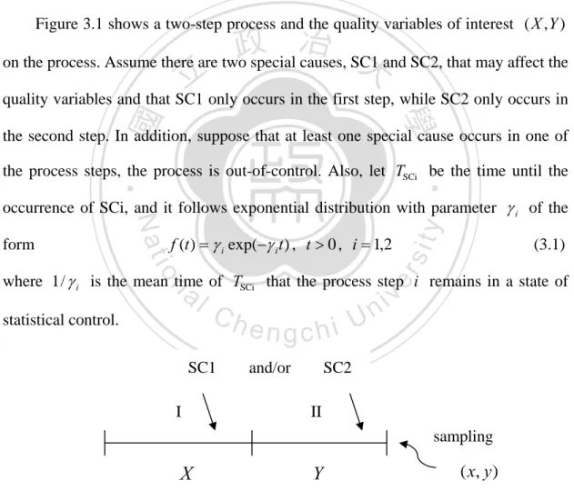
(18) 3. DESCRIPTION OF TWO DEPENDENT PROCESS STEPS Since there is not always a single step in an industrial process, discussion of the use of control charts for multiple process steps is required. Here, we consider a process with the two dependent steps. Let X be the quality measurement of interest for the first step and Y be the quality measurement of interest for the second step. The two steps of the process are dependent, with the second step affected by the first step. Furthermore, suppose that the values of X cannot be observed during the first step, but can be measured with Y at the end of the second step. Figure 3.1 shows a two-step process and the quality variables of interest ( X , Y ). 治政 on the process. Assume there are two special causes, SC1 大and SC2, that may affect the 立 quality variables and that SC1 only occurs in the first step, while SC2 only occurs in ‧ 國. 學. the second step. In addition, suppose that at least one special cause occurs in one of. ‧. the process steps, the process is out-of-control. Also, let TSCi be the time until the. y. (3.1). io. er. f (t ) = γ i exp(−γ i t ) , t > 0 , i = 1,2. form. sit. Nat. occurrence of SCi, and it follows exponential distribution with parameter γ i of the. where 1 / γ i is the mean time of TSCi that the process step i remains in a state of. n. al. statistical control.. Ch. SC1. engchi and/or. I. i Un. v. SC2 II sampling. X. Y. ( x, y ). Figure 3.1 Two-step process with the occurrence of SCi. 8.

(19) Assume X ~ N (μ X + δ 1σ X , (δ 2σ X ) 2 ) and that the target for the first step is express as T X = μ X − δ 3σ X , δ 3 ∈ R . When δ 3 = 0 , it implies TX = μ X . When the first step is in-control, δ 1 = 0 , δ 2 = 1 and δ 3 ∈ R ; otherwise, the first step has changed or drifted due to SC1. The constants δ1 , δ 2 and δ 3 represent the shift scales in the mean, the standard deviation and the target in the first step, respectively. Since the two process steps are dependent, and the second process step is affected by the first process step; i.e., the distribution of Y is affected by the distribution of X , then by following Wade and Woodall (1993), the relationship between Y and X may be expressed as the general form Y X = f ( X ) + ε . The variable ε is a random error,. 立. 政治大 and ε ~ NID (0, σ ) when 2. ε. the second step is. ‧ 國. 學. in-control. When X and Y have a simple linear relationship, and their absolute correlation coefficient is larger than 0.4, then we can use Zhang’s cause-selecting. ‧. control charts (1984) to monitor the second step correctly. The quality characteristic. sit. y. Nat. of the second process step should be specified by adjusting the effect of X on Y ;. n. al. er. io. i.e., the specific quality is presented by the cause-selecting values (or residuals),. i Un. v. e = Y X − Yˆ X , where Yˆ X is the fitted model of the paired observations ( x, y ). Ch. using a least square error method.. engchi. The distribution of the residual is e ~ N (δ 4σ e , (δ 5σ e ) 2 ), and the target for the second step is Te = 0 . When the second step is in-control, δ 4 = 0 , δ 5 = 1 and the process mean is equivalent to the target; otherwise, the second step has changed or drifted due to SC2. The constants δ 4 and δ 5 represent the shift scales in the mean and the standard deviation in the second step, respectively.. 9.

(20) 4. VARIABLE SAMPLING INTERVALS WEIGHTED LOSS CONTROL CHARTS 4.1 The Distributions of the VSI Weighted Loss Statistics. We now extend the VSI WL chart to monitor two dependent steps. In those charts, the first and second step weighted loss statistics are as follows.. WL1i = λ1 S X2 i + (1 − λ1 )( X i − TX ) 2. (4.1). WL2 i = λ2 S e2i + (1 − λ2 )e i. (4.2). n. n. Where X i =. ∑ X ij j =1. n. , S Xi = 2. 立. i = 1,2,..., m .. n. n. ∑( X ij − X i )2 j =1. 2. ∑ eij. = , e治 and n −政 1 n 大 i. j =1. S ei = 2. ∑ (e j =1. ij. − ei ) 2. n −1. ,. ‧ 國. 學. The WL1 chart is used for monitoring the increase in statistic WL1 in the first step, and the WL2 chart is used for monitoring the increase in statistic WL2 in the second. ‧. step. Monitor the increase in weighted loss statistics is equivalent to monitor the shifts. y. Nat. io. sit. in targets and variances. The weighted loss statistics for both steps cannot be. n. al. er. expressed by an exact distribution, but their cumulative distribution functions (CDF’s). Ch. i Un. v. can be derived to allow calculation of UCLs and UWLs of the proposed charts. We. engchi. denote F1 (⋅) is the CDF of statistic WL1 and F2 (⋅) is the CDF of statistic WL2 , and the CDF’s of the statistics WL1 and WL2 are derived in equations (4.3) and (4.4).. 10.

(21) F1 (m ; λ1 , δ 1 , δ 2 , δ 3 , n) ⎞ ⎛ (δ σ ) 2 (n − 1) S X2 ~ χ n2−1 ⎟⎟ = 1 − Pr ⎜⎜ λ1 S X2 + (1 − λ1 )( X − TX ) 2 > m | X ~ N ( μ X + δ 1σ X , 2 X ), 2 n (δ 2σ X ) ⎠ ⎝ ⎛ (δ σ ) 2 ⎞ m m or X > TX + | X ~ N ( μ X + δ 1σ X , 2 X ) ⎟⎟ − = 1 − Pr ⎜⎜ X < TX − 1 − λ1 1 − λ1 n ⎠ ⎝ 2 ⎞ ⎛ (δ σ ) 2 (n − 1) S X2 m − (1 − λ1 ) x − TX m m and S X2 > | X ~ N ( μ X + δ 1σ X , 2 X ), ~ χ n2−1 ⎟ Pr ⎜ TX − < X < TX + 2 ⎟ ⎜ 1 − λ1 1 − λ1 λ1 (δ 2σ X ) n ⎠ ⎝. (. ). ⎛ ⎛ (δ σ ) 2 ⎞ (δ σ ) 2 ⎞ m m = 1 − Pr ⎜⎜ x < T X − | X ~ N ( μ X + δ 1σ X , 2 X ) ⎟⎟ − Pr ⎜⎜ x > T X + | X ~ N ( μ X + δ 1σ X , 2 X ) ⎟⎟ 1 − λ1 n 1 − λ1 n ⎝ ⎠ ⎝ ⎠ m 1− λ1. TX +. ∫. −. m TX − 1− λ1. ⎛ ⎞ m − (1 − λ1 )( x − T X ) 2 (n − 1) S X2 Pr ⎜⎜ S X2 > | ~ χ n2−1 ⎟⎟ • f x d x 2 λ1 (δ 2σ X ) ⎝ ⎠. (). 政治大. n (T X −. io. al. n. TX +. m 1− λ1. ∫. − TX −. m 1− λ1. ⎧⎪ ⎨1 − Fχ n2−1 ⎪⎩. ⎟ ⎠. ⎞ m − μ X − δ 1σ X ) ⎟ 1 − λ1 ⎟ ⎟ δ 2σ X ⎟ ⎟ ⎠. y. Nat. ⎛ ⎞ ⎛ m ⎜ n (T X + ⎜ − μ X − δ 1σ X ) ⎟ 1 − λ1 ⎜ ⎟ ⎜ = Φ⎜ ⎟ − Φ⎜ Z < δ 2σ X ⎜ ⎟ ⎜ ⎜ ⎟ ⎜ ⎝ ⎠ ⎝. ]⎞⎟ • f (x ) d x. sit. m 1− λ1. TX −. [. ⎛ (n − 1) S X2 (n − 1) m − (1 − λ1 )( x − T X ) 2 Pr ⎜⎜ > 2 λ1 (δ 2σ X ) 2 ⎝ (δ 2σ X ). ‧. ∫. −. er. m 1− λ1. TX +. ‧ 國. 立. 學. ⎛ ⎞ ⎛ ⎞ m m ⎜ ⎜ n (T X − − μ X − δ 1σ X ) ⎟ n (T X + − μ X − δ 1σ X ) ⎟ 1 − λ1 1 − λ1 ⎜ ⎟ ⎜ ⎟ = 1 − Pr ⎜ Z < ⎟ − Pr ⎜ Z > ⎟ δ 2σ X δ 2σ X ⎜ ⎟ ⎜ ⎟ ⎜ ⎟ ⎜ ⎟ ⎝ ⎠ ⎝ ⎠. ni Cλ h)( x − T ) ]⎞⎫⎪ ⎛ (n − 1)[m − (1 − U ⎜ e n g⎟⎟⎬⎪c• hf (xi) d x ⎜ λ (δ σ ) ⎝ ⎠⎭. v. 2. X. 1. 2. 1. 2. X. Since TX = μ X − δ 3σ X , δ 3 ∈ R F1 (m ; λ1 , δ 1 , δ 2 , δ 3 , n) ⎛ m ⎜ n( − δ 1σ X − δ 3σ X 1 − λ1 ⎜ = Φ⎜ δ 2σ X ⎜ ⎜ ⎝ μ X −δ 3σ X +. −. ∫. m 1− λ1. m μ X −δ 3σ X − 1− λ1. ⎞ ⎛ ⎞ m ⎜ − n( + δ 1σ X + δ 3σ X ) ⎟ )⎟ 1 − λ1 ⎟ ⎜ ⎟ ⎟ − Φ⎜ ⎟ δ 2σ X ⎟ ⎜ ⎟ ⎟ ⎜ ⎟ ⎠ ⎝ ⎠. [. ]. ⎧⎪ ⎛ (n − 1) m − (1 − λ1 )( x − μ X + δ 3σ X ) 2 ⎞⎫⎪ ⎟⎬ • f x d x ⎨1 − Fχ n2−1 ⎜⎜ ⎟⎪ λ1 (δ 2σ X ) 2 ⎪⎩ ⎝ ⎠⎭. (). Where f x is the pdf of X and X ~ N ( μ X + δ 1σ X ,. 11. (). (δ 2σ X ) 2 ). n. (4.3).

(22) F2 (m ; λ 2 , δ 4 , δ 5 , n) ⎛ ⎞ 2 (δ σ ) 2 (n − 1) S e2 = 1 − Pr ⎜⎜ λ2 S e2 + (1 − λ2 )e > m | e ~ N (δ 4σ e , 5 e ), ~ χ n2−1 ⎟⎟ 2 n (δ 5σ e ) ⎝ ⎠ ⎛ (δ σ ) 2 ⎞ m m = 1 − Pr ⎜⎜ e < − or e > | e ~ N (δ 4σ e , 5 e ) ⎟⎟ − 1 − λ2 1 − λ2 n ⎝ ⎠ 2 ⎛ ⎞ (δ σ ) 2 (n − 1) S e2 m m m − (1 − λ2 )e 2 ⎟ <e< and S e2 > | e ~ N (δ 4σ e , 5 e ), ~ χ Pr ⎜ − n −1 ⎜ ⎟ 1 − λ2 1 − λ2 λ2 (δ 5σ e ) 2 n ⎝ ⎠ ⎛ ⎛ (δ σ ) 2 ⎞ (δ σ ) 2 ⎞ m m | e ~ N (δ 4σ e , 5 e ) ⎟⎟ − Pr ⎜⎜ e > | e ~ N (δ 4σ e , 5 e ) ⎟⎟ = 1 − Pr ⎜⎜ e < − 1 − λ2 n 1 − λ2 n ⎠ ⎝ ⎠ ⎝. 立. ⎛ m ⎜ n( − δ 4σ e 1 − λ2 ⎜ = Φ⎜ δ5σ e ⎜ ⎜ ⎝. ]⎞⎟ • f (e) d e ⎟ ⎠. i. e. m 1− λ2. i Un. v. n gmc h ⎞ ⎛ ⎞ ⎜ − n( + δ 4σ e ) ⎟ )⎟ 1 − λ2 ⎟ ⎜ ⎟ ⎟ − Φ⎜ ⎟ δ5σ e ⎟ ⎜ ⎟ ⎟ ⎜ ⎟ ⎠ ⎝ ⎠. ⎧⎪ ⎛ (n − 1) m − (1 − λ )e 2 2 ⎨1 − Fχ n2−1 ⎜⎜ 2 λ2 (δ 5σ e ) ⎪⎩ ⎝. ∫. −. Ch. [. m 1− λ2. −. al. ⎞ m − δ 4σ e ) ⎟ 1 − λ2 ⎟ ⎟ δ5σ e ⎟ ⎟ ⎠. n. m 1− λ2. n(. ‧. −. [. ⎛ (n − 1) S 2 (n − 1) m − (1 − λ )e 2 e 2 Pr ⎜ > 2 ⎜ (δ 5σ e ) 2 ( ) λ δ σ 2 5 e ⎝. io. ∫. −. ⎛ ⎞ m ⎜ − δ 4σ e ) ⎟ 1 − λ2 ⎜ ⎟ ⎟ − Pr ⎜ Z > δ5σ e ⎜ ⎟ ⎜ ⎟ ⎝ ⎠. Nat. m 1− λ2. n (−. 學. ⎛ ⎜ ⎜ = 1 − Pr ⎜ Z < ⎜ ⎜ ⎝. y. m 1− λ2. sit. −. 政治 (大). 2 ⎞ ⎛ m − (1 − λ 2 )e (n − 1) S e2 Pr ⎜ S e2 > | ~ χ n2−1 ⎟ • f e d e 2 ⎟ ⎜ λ2 (δ 5σ e ) ⎠ ⎝. er. ∫. −. ‧ 國. m 1− λ2. (). ]⎞⎟⎫⎪⎬ • f (e) d e ⎟⎪ ⎠⎭. (δ 5σ e ) 2 Where f e is the pdf of e and e ~ N (δ 4σ e , ). n. 12. (4.4).

(23) 4.2 Design of the VSI Weighted Loss Control Charts. Because the statistics WL1 and WL2 are non-negative, two LCLs are set to zero. The structure of the VSI WL1 and WL2 control charts under in-control distribution is as follows (see Figure 4.1).. Figure 4.1 The structure of VSI WL1 and WL2 charts. 政治大. Here, we divide the VSI WL1 and WL2 control charts into three regions. Let. 立. the central region be I i1 = (0,UWLi ) , warning region be I i 2 = (UWLi ,UCLi ) and. ‧ 國. 學. control region be I i 3 = (0, UCLi ) of the VSI WL1 and WL2 charts, i = 1,2 . From. ‧. the CDF of statistics WL1 and WL2 in equations (4.3) and (4.4), the UCL1 and. n. al. i Un. UCL2 = F2−1 (1 − α ; δ 4 = 0, δ 5 = 1). Ch. engchi. (4.5). er. io. UCL1 = F1−1 (1 − α ; δ 1 = 0, δ 2 = 1, δ 3 ). sit. y. Nat. UCL2 can be calculated by equations (4.5) and (4.6) given λ1 , λ 2 and δ 3 .. v. (4.6). Since using the two VSI WL1 and WL2 control charts, three variable sampling intervals, t q , q = 1,2,3 , are adopted, 0< t1 < t 2 < t 3 < ∞ . The choice of t q for the next sample depend on the position of the statistics WL1 and WL2 . If the sample points for WL1 and WL2 charts fall within the interval I 11 and I 21 , then the next sampling interval should be long ( t3 ). If the sample points for WL1 and WL2 charts fall within the interval I 11 and I 22 or I12 and I 21 , then the next sampling interval should be median ( t 2 ). If the sample points for WL1 and WL2 charts fall within the interval I12 and I 22 , then the next sampling interval should be short ( t1 ). The relationship between the next sampling interval and the position of the current 13.

(24) samples can be expressed as follows.. ⎧t3 , if WL1 ∈ I11 , WL2 ∈ I 21 ⎪t , if WL ∈ I , WL ∈ I ⎪ 1 11 2 22 tq = ⎨ 2 ⎪t 2 , if WL1 ∈ I12 , WL2 ∈ I 21 ⎪⎩t1 , if WL1 ∈ I12 , WL2 ∈ I 22. (4.7). To compare the performance of VSI and FP charts, we should demand the same average sampling interval under the in-control period.. t 3 p 01 + t 2 p02 + t 2 p03 + t1 p 04 = t 0. (4.8). 政治大 = P (0 < WL < UWL | 0 < WL < UCL , δ = 0, δ = 1, δ ) 立 • P(0 < WL < UWL | 0 < WL < UCL , δ = 0, δ = 1). Where. p01. 1. 1. 2. 1. 2. 1. 2. 2. 4. 3. 5. 學. ‧ 國. 2. 1. ⎛ F (UWL1 ; δ1 = 0, δ 2 = 1, δ 3 ) ⎞ ⎛ F2 (UWL2 ; δ 4 = 0, δ 5 = 1) ⎞ ⎟⎟ • ⎜⎜ ⎟⎟ = ⎜⎜ 1 ⎝ F1 (UCL1 ; δ1 = 0, δ 2 = 1, δ 3 ) ⎠ ⎝ F2 (UCL2 ; δ 4 = 0, δ 5 = 1) ⎠. y. ‧. Nat. p02 = P(UWL1 < WL1 < UCL1 | 0 < WL1 < UCL1 , δ1 = 0, δ 2 = 1, δ 3 ). io. sit. • P(0 < WL2 < UWL2 | 0 < WL2 < UCL2 , δ 4 = 0, δ 5 = 1). n. er. ⎛ F (UWL1 ; δ1 = 0, δ 2 = 1, δ 3 ) ⎞ ⎛ F2 (UWL2 ; δ 4 = 0, δ 5 = 1) ⎞ ⎟⎟ • ⎜⎜ ⎟⎟ = ⎜⎜1 − 1 ⎝ F1 (UCL1 ; δ1 = 0, δ 2 = 1, δ 3 ) ⎠ ⎝ F2 (UCL2 ; δ 4 = 0, δ 5 = 1) ⎠. al. Ch. engchi U. (4.9). v ni. (4.10). p03 = P(0 < WL1 < UWL1 | 0 < WL1 < UCL1 , δ1 = 0, δ 2 = 1, δ 3 ). • P(UWL2 < WL2 < UCL2 | 0 < WL2 < UCL2 , δ 4 = 0, δ 5 = 1) ⎛ F (UWL1 ; δ1 = 0, δ 2 = 1, δ 3 ) ⎞ ⎛ F2 (UWL2 ; δ 4 = 0, δ 5 = 1) ⎞ ⎟⎟ • ⎜⎜1 − ⎟⎟ = ⎜⎜ 1 ⎝ F1 (UCL1 ; δ1 = 0, δ 2 = 1, δ 3 ) ⎠ ⎝ F2 (UCL2 ; δ 4 = 0, δ 5 = 1) ⎠. (4.11). p04 = P(UWL1 < WL1 < UCL1 | 0 < WL1 < UCL1 , δ1 = 0, δ 2 = 1, δ 3 ). • P(UWL2 < WL2 < UCL2 | 0 < WL2 < UCL2 , δ 4 = 0, δ 5 = 1). ⎛ F (UWL1 ; δ 1 = 0, δ 2 = 1, δ 3 ) ⎞ ⎛ F2 (UWL2 ; δ 4 = 0, δ 5 = 1) ⎞ ⎟⎟ • ⎜⎜1 − ⎟⎟ = ⎜⎜1 − 1 ⎝ F1 (UCL1 ; δ1 = 0, δ 2 = 1, δ 3 ) ⎠ ⎝ F2 (UCL2 ; δ 4 = 0, δ 5 = 1) ⎠. = 1 − p01 − p02 − p03. (4.12) 14.

(25) Following Costa (1997), the first sampling interval is chosen randomly when the process is starting. When the process is in-control, all sampling intervals, including the first one, should have a probability of p01 of being t3 , a probability of p02 + p03 4. ∑p. of being t 2 and a probability of p04 of being t1 , where. i =1. 0i. = 1.. According to Costa (1998), to facilitate the computation of the performance measures, during the in-control period the conditional probability of a sample point falling in the central region (or the warning region), given that it falls in the control region, is the same for both the WL1 and WL2 charts. That is,. 政治大 < UWL | 0 < WL < UCL , δ 立. P (0 < WL1 < UWL1 | 0 < WL1 < UCL1 , δ 1 = 0, δ 2 = 1, δ 3 ) = P (0 < WL 2. 2. 2. 4. = 0, δ 5 = 1). F1 (UWL1 ; δ1 = 0, δ 2 = 1, δ 3 ) F2 (UWL2 ; δ 4 = 0, δ 5 = 1) = F1 (UCL1 ; δ1 = 0, δ 2 = 1, δ 3 ) F2 (UCL2 ; δ 4 = 0, δ 5 = 1). ‧ 國. ‧. The procedure to derive the warning limits is as follows.. y. Nat. sit. Step1. From equation (4.13), we let. er. F1 (UWL1; δ1 = 0, δ 2 = 1, δ 3 ) F2 (UWL2 ; δ 4 = 0, δ 5 = 1) = F1 (UCL1 ; δ1 = 0, δ 2 = 1, δ 3 ) F2 (UCL2 ; δ 4 = 0, δ 5 = 1). io. A=. (4.13). 學. ⇒. 2. al. n. iv n C , (1 − A) A = p From equations (4.9) to (4.12), wehobtain e n gAc h= pi U 2. 01. 02. , A(1 − A) = p03. and (1 − A) 2 = p04 Step2. Put the results of step1 in equation (4.8), and we can obtain A=. − 2(t 2 − t1 ) ± 4(t 2 − t1 ) 2 − 4(t1 − 2t 2 + t 3 )(t1 − t 0 ) 2(t1 − 2t 2 + t 3 ). (4.14). Step3. Specify t 0 , t1 , t 2 , t 3 , then A can be determined from equation (4.14). Step4. Specify λ1 , λ2 , δ 3 , A , then UWL1 and UWL2 can be determined as follows. −1. UWL1 = F1 ( A • (1 − α ) ; δ 1 = 0, δ 2 = 1, δ 3 ) −1. UWL2 = F2 ( A • (1 − α ) ; δ 4 = 0, δ 5 = 1) 15. (4.15) (4.16).

(26) 4.3 Performance Measurement for VSI Weighted Loss Control Charts. To compare performance of VSI and FP charts, the adjusted average time to signal (AATS) is used as performance criteria. The smaller AATS, the better performance of the proposed charts. The AATS is the mean time the process remains out-of-control. Since. TSCi ~ exp(γ i ) , i = 1, 2 ,. thus. T(1) ~ exp(γ1 + γ2 ) ,. where. T(1) = min(TSC1 , TSC2 ) is the occurrence time until the first special cause occurs. Hence,. AATS = ATC −. 1 γ1 + γ2. (4.17). The average time of the cycle (ATC) is the average time from the process starts. 治政 until the first true signal occurs. The memory-less大 property of the exponential 立 distribution allows the computation of the ATC through a Markov chain approach. ‧ 國. 學. We use the Markov chain approach to derive the AATS, and all possible process. ‧. states for using VSI WL1 and WL2 charts must be defined. After each sampling,. y. Nat. one of these possible states is reached according to the occurrence of the special cause. er. io. sit. and the location of the sample points in WL1 and WL2 charts. The control charts. al. produce a signal when at least one of the sample points fall outside the control limits.. n. iv n C Table 4.1 shows the 22 possible states, which can be classified into h e nprocess gchi U. transient and absorbing states based on Markov property. State 1-21 are transient states since they may transit to other states, while state 22 is an absorbing state since it cannot transit to any other state. After define all possible states at each end of the sampling time, the transition probability from state i to state j with variable sampling intervals t q , Pi , j (t q ) can be calculated.. 16.

(27) For example, P1,3 ( t 3 ) = P(TSC1 < t 3 ) • P(TSC2 > t 3 ) • P(WL1 ∈ I 11 , WL2 ∈ I 21 ) = (1 − e −γ 1t3 ) • e −γ 2t3 • F1 ( UWL1 ; δ 1 ≠ 0, δ 2 > 1, δ 3 ) • F2 ( UWL2 ; δ 4 = 0, δ 5 = 1). P11,16 ( t2 ) = P(TSC2 < t2 ) • P(WL1 ∈ I12 ,WL2 ∈ I 22 ). = (1 − e −γ 2 t 2 ) • (F1 ( UCL1;δ1 ≠ 0, δ 2 > 1, δ 3 ) − F1 ( UWL1;δ1 ≠ 0, δ 2 > 1, δ 3 ) ) •. (F2 ( UCL2 ;δ 4 ≠ 0,δ 5 > 1) − F2 ( UWL2 ;δ 4 ≠ 0,δ 5 > 1) ). The transition probability from state i to state j can be express by a square matrix ⎡Q A ⎤ P=⎢ ⎥ ,where Q 21× 21 is the transition probability matrix with each element ⎣ 0 1⎦ expresses the transition. 政治大 probability from transient state 立. i to transient state j ,. ‧ 國. 學. Pi , j (t q ) , i = 1,..., 21, j = 1,..,21, q = 1,2,3 . A ' = (P1, 22 , P2, 22 ,..., P21, 22 )1×21 , where Pi , 22 is. the probability of transient state i to absorbing state 22. 01×21 is vector with all. ‧. elements being zero and 11×1 is the probability 1 for staying absorbing state 22. From. y. Nat. iv n C ,0,0,0, ph,0,0,0, p ,0,0,0,0U e n g c h i ,0,0,0,0). n Where b' = ( p 01 ,0,0,0, p 02. er. io. al. ATC = b' (I − Q) −1 t. sit. the elementary properties of Markov chains (Cinlar, 1975), the ATC is derived as. 03. 04. (4.18) is a (1×21) vector. with the starting probability for transient state i , i = 1,...,21 I is the identity matrix of order 21 * * , t 21 ) is a (21× 1) t ' = (t3 , t3 , t3 , t3 , t 2 , t 2 , t 2 , t 2 , t 2 , t 2 , t 2 , t 2 , t1 , t1 , t1 , t1 , t17* , t18* , t19* , t 20. vector of sampling interval time for transient state i , i = 1,...,21 , where * t17* ~ t 21 are the average sampling interval of state 17-21.. 17.

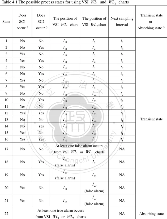
(28) Table 4.1 The possible process states for using VSI WL1 and WL2 charts. occur ?. occur ?. 1. No. 2. VSI WL1 chart. VSI WL2 chart. interval. No. I11. I 21. t3. No. Yes. I11. I 21. t3. 3. Yes. No. I11. I 21. t3. 4. Yes. Yes. I11. I 21. t3. 5. No. No. I 12. I 21. t2. 6. No. Yes. I 12. I 21. t2. 7. Yes. No. I 12. I 21. t2. 8. Yes. Yes. 12. 21. t2. 9. No. No. 治 I I 政大 I I 11. 22. t2. 10. No. Yes. I11. I 22. t2. 11. Yes. No. I11. I 22. 12. Yes. Yes. I11. I 22. 13. No. No. I 12. I 22. t1. 14. No. Yes. I 12. I 22. 15. Yes. No. I 12. I 22. t1. 16. Yes. Yes. I 12. I 22. t1. 17. No. No. io. er. 立. ‧ 國. State. At least one false alarm occurs. n. a l from VSI WL or WL chartsi v n C hI e n g c h i IU 1. No. Yes. 19. No. Yes. 20. Yes. No. I11. 21. Yes. No. I 12. (false alarm). I13 (false alarm). or Absorbing state ?. t2 t2 Transient state. t1. NA. 21. NA. I 22. NA. I 23 (false alarm). I 23 (false alarm). At least one true alarm occurs from VSI WL1 or WL2 charts. 18. Transient state. 2. 13. 18. 22. 學. Next sampling. y. SC2. The position of. sit. SC1. The position of. ‧. Does. Nat. Does. NA NA NA. Absorbing state.

(29) 4.4 An example of VSI Weighted Loss Control Charts To explain the application of our proposed VSI WL1 and WL2 control charts for two dependent process steps, an example is illustrated. Consider the data used by Montgomery (2009), “Introduction to Statistical Quality Control, 6th Edition,” Table 11-5, pp.514. We use the variables x9 and y1 as paired data ( X , Y ) . Since the original data is not enough, the 150 data is duplicated by the original data. Based on the data analyses, both variables. X. and Y. have normal. distributions. Their relationship of Y and X can be expressed by a linear regression model and the cooefficient of correlation is 0.845. The fitted linear. 治政 regression model for the 150 paired data is 大立 ‧ 國. 學. Yˆ X = 853 .256 + 89.57 X. (4.19). The fitted regression model with significant coefficients and an R2(adj)=71.1%. Thus,. ‧. the residual ( e ) is obtained by Y X − Yˆ X . The estimated in-control means and. y. Nat. al. er. io. sit. standard deviations of X and e are μˆ *X = 1.1025 , σˆ *X = S X C4 = 0.0077 , μˆ e* = 0. n. and σˆ e* = MSE = 0.502 , respectively. In order to simply the calculation, we. Ch. engchi. i Un. v. standardize the distribution of X and e , and let μˆ X = 0 , σˆ X = 1 , σˆ e = 1 . We assume SC1 and SC2 follow exponential distributions with parameters γ1 = 0.05 and γ 2 = 0.1 , and the mean and the variance for the first step would shift to μˆ X + 0.5σˆ X. and (1.5σˆ X ) ,and the mean and the variance for the second step would shift to 2. μˆ e + 0.5σˆ e and (2.5σˆ e ) . We also set TX = μˆ X , which means δ 3 = 0 . 2. Since it is not easy to specify optimal variable parameters, an optimization technique is used to determine the optimum variable parameters for minimum AATS. Hence, the mathematical expression for the optimum VSI WL1 and WL2 control. 19.

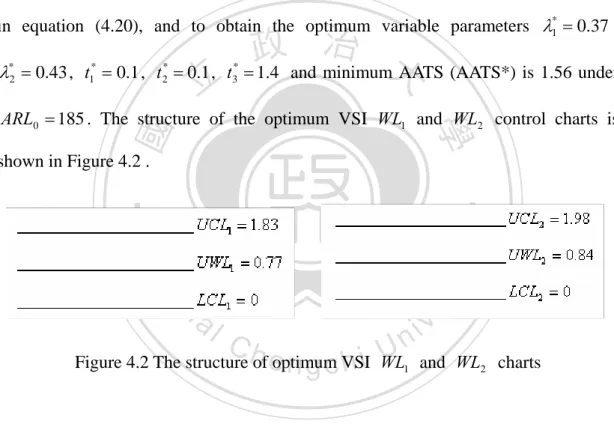
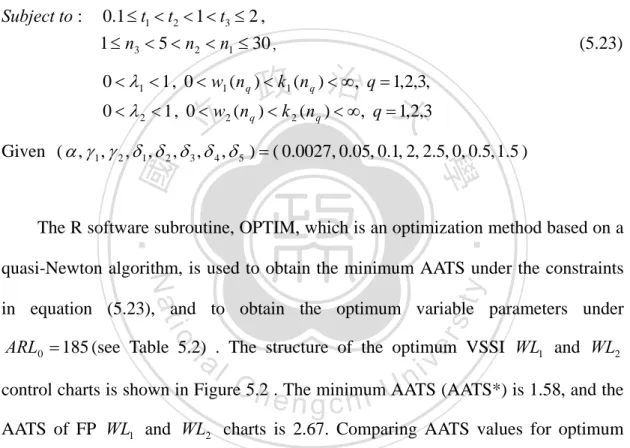
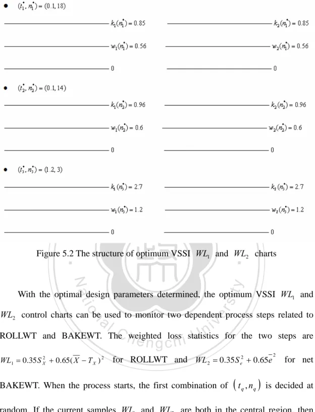
(30) charts is Objective function : Minimize AATS. 0.1 ≤ t1 < t 2 < 1 < t3 ≤ 2 , 0 < λ1 < 1 , 0 < UWL1 < UCL1 < ∞ ,. Subject to :. (4.20) 0 < λ 2 < 1 , 0 < UWL2 < UCL2 < ∞ , Given ( n, α , γ 1 , γ 2 , δ 1 , δ 2 , δ 3 , δ 4 , δ 5 ) = ( 5, 0.0027, 0.05, 0.1, 0.5, 1.5, 0, 0.5, 2.5 ). The R software subroutine, OPTIM, which is an optimization method based on a quasi-Newton algorithm, is used to obtain the minimum AATS under the constraints in equation (4.20), and to obtain the optimum variable parameters λ1* = 0.37 ,. λ = 0.43 , t = 0.1 , t = 0.1 , t * 2. * 1. * 2. 立. * 3. 政治大 = 1.4 and minimum AATS (AATS*) is 1.56 under. ‧ 國. 學. ARL0 = 185 . The structure of the optimum VSI WL1 and WL2 control charts is. shown in Figure 4.2 .. ‧. n. er. io. sit. y. Nat. al. Ch. engchi. i Un. v. Figure 4.2 The structure of optimum VSI WL1 and WL2 charts. With the optimal design parameters determined, the optimum VSI WL1 and WL2 control charts can be used to monitor two dependent process steps. The. weighted loss statistics for the two steps are WL1 = 0.37 S X2 + 0.63( X − T X ) 2 for the first step and WL 2 = 0.43 S e2 + 0.57 e. 2. for the second step. When the process starts, the. first sampling interval is decided at random. If the current samples WL1 and WL2 are both in the central region, next sampling interval t3* = 1.4 is adopted; however, if one of the current samples is in the central region and the other is in the warning 20.

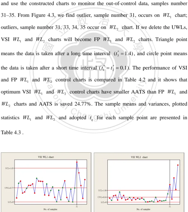
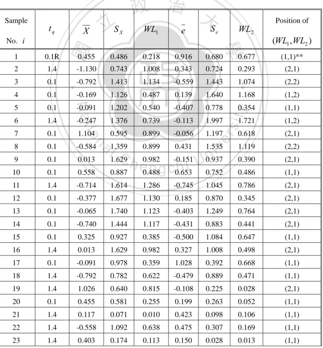
(31) region ,or both samples are in the warning region, next sampling interval t1* = t 2* = 0.1 is adopted. If at least one samples fall outside the control limits, stop sampling and search and repair the special cause. After the special cause is repaired, the next sampling interval is chosen at random. The 30 samples of (WL1 , WL2 ) are all within the control regions, so we can use the constructed VSI WL1 and WL2 control charts to monitor the process. We generate 25 paired out-of-control data with X ~ N ( 0.5, 1.5 2 ) and e ~ N ( 0.5, 2.5 2 ) , and use the constructed charts to monitor the out-of-control data, samples number 31–35. From Figure 4.3, we find outlier, sample number 31, occurs on WL1 chart;. 治政 chart. If we delete the UWLs, outliers, sample number 31, 33, 34, 35 occur on WL 大立 VSI WL and WL charts will become FP WL and WL charts. Triangle point 2. 2. 1. 2. 學. ‧ 國. 1. means the data is taken after a long time interval (t3* = 1.4) , and circle point means. ‧. the data is taken after a short time interval ( t1* = t 2* = 0.1 ). The performance of VSI. sit. y. Nat. and FP WL1 and WL2 control charts is compared in Table 4.2 and it shows that. n. al. er. io. optimum VSI WL1 and WL2 control charts have smaller AATS than FP WL1 and. v. WL2 charts and AATS is saved 24.77%. The sample means and variances, plotted. Ch. engchi. i Un. statistics WL1 and WL2 and adopted t q for each sample point are presented in Table 4.3 .. VSI WL1 chart. VSI WL2 chart. UCL=1.83. UWL=0.77 UCL=1.98 UWL=0.84. LCL=0. LCL=0. 31. 31. No. of sam ples. No. of sam ples. Figure 4.3 Optimum VSI WL1 and WL2 charts for monitoring the first and second steps 21.

(32) Table 4.2 Performance comparison between optimum VSI and FP WL1 and WL2 charts Outliers ( Sample No. i ). Optimum VSI. For the. For the. first step. second step. 31(m)*. WL1 and WL2 charts FP WL1 and WL2 charts. Saved AATS (%). 31(v)*、33(v)、 34(v)、35(v) 31(v)、33(v)、. 31(m). 24.77%. 34(v)、35(v). * The out-of-control reason from sample number 31 is the mean shift in the first step and the variance shift in the second step.. Table 4.3 The plotted statistics and adopted. tq. 3. 0.1. 4. 0.1. 5. 0.1. 6. Se. WL2. Position of. (WL1 , WL2 ). 0.455. 0.486. 0.218. 0.916. 0.680. 0.677. (1,1)**. -1.130. 0.743. 1.008. 0.343. 0.724. 0.293. (2,1). -0.792. 1.413. 1.134. -0.559. 1.443. -0.169. 1.126. 0.487. 0.139. 1.640. -0.091. 1.202. 0.540. -0.407. 0.778. 1.4. -0.247. 1.376. 0.739. -0.113. 1.997. 7. 0.1. 1.104. 0.595. 0.899. -0.056. 1.197. 8. 0.1. -0.584. 0.899. 0.431. 9. 0.1. 0.013. 10. 0.1. 0.558. 11. 1.4. -0.714. 1.614. 1.286. -0.745. 12. 0.1. -0.377. 1.677. 1.130. 13. 0.1. -0.065. 1.740. 14. 0.1. -0.740. 15. 0.1. 16. 1.074. (2,2). 1.168. (1,2). 0.354 1.721. (1,2). 0.618. (2,1). 1.535. 1.119. (2,2). 0.982 -0.151 U0.937 e0.488 h i 0.752 n g c0.653. 0.390. (2,1). 0.486. (1,1). 1.045. 0.786. (2,1). 0.185. 0.870. 0.345. (2,1). 1.123. -0.403. 1.249. 0.764. (2,1). 1.444. 1.117. -0.431. 0.883. 0.441. (2,1). 0.325. 0.927. 0.385. -0.500. 1.084. 0.647. (1,1). 1.4. 0.013. 1.629. 0.982. 0.327. 1.008. 0.498. (2,1). 17. 0.1. -0.091. 0.978. 0.359. 1.028. 0.392. 0.668. (1,1). 18. 1.4. -0.792. 0.782. 0.622. -0.479. 0.889. 0.471. (1,1). 19. 1.4. 1.026. 0.640. 0.815. -0.108. 0.225. 0.028. (2,1). 20. 0.1. 0.455. 0.581. 0.255. 0.199. 0.263. 0.052. (1,1). 21. 1.4. 0.117. 0.071. 0.010. 0.423. 0.098. 0.106. (1,1). 22. 1.4. -0.558. 1.092. 0.638. 0.475. 0.307. 0.169. (1,1). 23. 1.4. 0.403. 0.174. 0.113. 0.150. 0.028. 0.013. (1,1). n. a l1.359 Ch 1.629 0.887. 22. er. (1,1). io. y. 1.4. e. sit. 2. WL1. ‧. 0.1R. X. Nat. 1. 政治大. 學. No. i. 立S. X. ‧ 國. Sample. t q for example of optimum VSI WL1 and WL2 charts. v ni.

(33) 24. 1.4. 1.078. 0.348. 0.777. -0.738. 1.086. 0.817. (2,1). 25. 0.1. -0.740. 1.476. 1.152. -0.391. 0.081. 0.090. (2,1). 26. 0.1. 0.532. 0.427. 0.246. -0.666. 0.150. 0.262. (1,1). 27. 1.4. 0.169. 0.213. 0.035. -0.285. 0.580. 0.191. (1,1). 28. 1.4. -0.429. 1.250. 0.694. 0.217. 0.703. 0.239. (1,1). 29. 1.4. 0.013. 0.071. 0.002. -0.669. 0.230. 0.278. (1,1). 30. 1.4. 1.078. 0.266. 0.758. 1.215. 1.127. 1.387. (1,2). Monitor sample from No. 31-35 Sample. tq. X. SX. WL1. Se. e. WL2. Position of. (WL1 , WL2 ). No. i 31. 0.1. 1.500. 1.418. 2.161. -0.333. 2.588. 2.942. (3,3). 32. 0.1R. 1.368. 1.048. 1.585. 0.102. 1.106. 0.532. (2,1). 33. 0.1. 1.049. 4.081. (2,3). 34. 0.1R. 0.074. 2.131. (1,3). 35. 0.1R. 0.898. 0.394 3.047 治 0.720 政 0.196 1.254 1.695 大立1.380 1.213 1.215 3.552. 6.266. (2,3). 0.741. t q randomly ;. 1234：out-of-control sample. 學. ‧ 國. R：choose the next combination of. 0.897. **1 represents the sample point fall in the central region; 2 represents the sample point fall in the warning region;. ‧. 3 represents the sample point beyond the control region.. y. Nat. io. sit. We also compare the detection ability of optimum VSI WL1 and WL2 control. al. n. X. er. charts and FP Z X − Z S 2 and Z e − Z S 2 control charts. It shows that FP Z X − Z S 2 e. Ch. engchi U. v ni. X. and Z e − Z S 2 control charts can not detect the outlier, sample number 34, in the e. second step, and optimum VSI WL1 and WL2 charts have smaller AATS and out-of-control average loss per unit product than FP Z X − Z S 2 and Z e − Z S 2 charts X. e. and AATS is saved 34.34% and loss is saved 48.22% (see Figure 4.4 and Table 4.4). The out-of-control average loss per unit product for WL1 and WL2 charts and for FP Z X − Z S 2 and Z e − Z S 2 charts can be expressed in equations (4.21) and (4.22). e. X. WL1 + WL 2 = λ1 (δ 2 S X ) 2 + (1 − λ1 )(δ 1 S X + δ 3 S X ) 2 + λ 2 (δ 5 S e ) 2 + (1 − λ 2 )(δ 4 S e ) 2. = λ1δ 2 + (1 − λ1 )(δ 1 + δ 3 ) 2 + λ 2δ 5 + (1 − λ 2 )δ 4 2. 2. 23. 2. (4.21).

(34) 2 2 2 2 LS = L X + LS 2 + Le + LS 2 = (δ 1 S X ) 2 + (δ 2 S X ) 2 + (δ 4 S e ) 2 + (δ 5 S e ) 2 = δ 1 + δ 2 + δ 4 + δ 5 (4.22) X. e. ( n = 5, t = 1, UCLX = 3.2, UCLS = 17.8, UCLe = 3.2, UCLS = 17.8 under ARL0 = 185 ) 2 X. 2 e. Z(X-bar) chart. Z(Sx^2) chart. UCL=3.2. UCL=17.8. CL=0. LCL=-3.2 LCL=0. 31. 31. No. of sam ples. No. of sam ples. 政治大. Z(e-bar) chart UCL=3.2. 立. Z(Se^2) chart. LCL=-3.2. 學. ‧ 國. CL=0. UCL=17.8. LCL=0. ‧. 31. 31. No. of sam ples. No. of sam ples. y. charts for monitoring the first and second steps. sit. io. n. al. 2 e. er. Nat. Figure 4.4 FP Z X − Z S 2 and Z e − Z S X. Ch. i Un. v. Table 4.4 Performance comparison between optimum VSI WL1 and WL2 charts and FP Z X − Z S 2 and Z e − Z S X. 2 e. charts. engchi. Outliers (Sample No. i ). Optimum VSI. WL1 and WL2 charts. For the. For the. first step. second step. 31(m). FP Z X − Z S 2. X. 31(m) and Z e − Z S. 2 e. charts. Saved. Saved. AATS (%). loss (%). 34.34%. 48.22%. 31(v)、33(v)、 34(v)、35(v). 31(v)、 33(v)、35(v). 24.

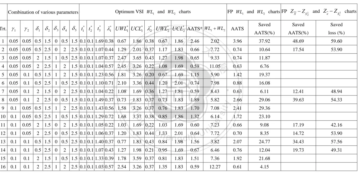
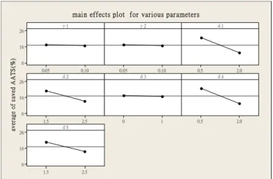
(35) 4.5 Performance Comparison for VSI Weighted Loss Control Charts Consider the levels of the process parameters to be : γ 1 = (0.05, 0.1) , γ 2 = (0.05, 0.1) , δ 1 = (0.5, 2) , δ 2 = (1.5, 2.5), δ 3 = (0, 1), δ 4 = (0.5, 2) and δ 5 = (1.5, 2.5) .. To investigate the effects of the parameters (γ 1 , γ 2 , δ 1 , δ 2 , δ 3 , δ 4 , δ 5 ) on AATS and the out-of-control average loss per unit product, and to compare the performances among optimum VSI WL1 and WL2 charts, FP WL1 and WL2 charts and FP Z X − Z S 2 and Z e − Z S 2 charts, we adopted 16 combinations of these parameters e. X. using an orthogonal array table L16 (27).. 政治大 determined using an optimization 立. Here, the optimal variable sampling intervals and weighted factors for the proposed charts are. technique, the OPTIM. ‧ 國. 學. subroutine in R program to minimize AATS under the following constraints. That is, Objective function : Minimize AATS. ‧. Subject to :. y. Nat. 0.1 ≤ t1 < t2 < 1 < t3 ≤ 2 , 0 < λ1 < 1 , 0 < UWL1 < UCL1 < ∞,. n. al. sit. (4.23). er. io. 0 < λ2 < 1 , 0 < UWL2 < UCL2 < ∞. i Un. v. The optimum results are shown in Table 4.5. The results indicate that optimum VSI. Ch. engchi. WL1 and WL2 charts use less time than FP WL1 and WL2 charts, and the AATS is. saved from 4.15% to 37.92%. Under δ 3 = 0 , optimum VSI WL1 and WL2 charts also save time and result in less loss than FP Z X − Z S 2 and Z e − Z S 2 charts, and X. e. the AATS savings from 12.41% to 48.69% and loss saving from 42.16% to 59.6%. We also created main effects plots for the saved AATS and loss percentages versus various parameters within the optimized VSI WL1 and WL2 charts. There were three main results in those plots: 1. Figure 4.5 indicates that parameters δ 1 , δ 2 , δ 4 and δ 5 are significant, and optimum VSI WL1 and WL2 charts would save more AATS percentage than FP 25.

(36) WL1 and WL2 charts when the two dependent process means and variances both. have small shifts. However, parameters γ 1 , γ 2 and δ 3 are not significant for saved AATS percentage. 2. Figure 4.6a indicates that parameters γ 1 , δ 1 , δ 2 , δ 4 and δ 5 are significant, when. γ 1 , δ 1 , δ 2 , δ 4 , δ 5 decrease, optimum VSI WL1 and WL2 charts would save more AATS percentage than FP Z X − Z S 2 and Z e − Z S 2 charts. e. X. 3. Figure 4.6b indicates parameters δ 1 and δ 4 are significant, when δ 1 and δ 4 decrease, optimum VSI WL1 and WL2 charts would save more loss percentage. 政治大. than FP Z X − Z S 2 and Z e − Z S 2 charts. X. 立. e. ‧ 國. 學. From the results of the optimum-parameter data analyses, we conclude that the charts is better than FP WL1 and. ‧. performance of optimum VSI WL1 and WL2 e. sit. X. y. Nat. WL2 charts and FP Z X − Z S 2 and Z e − Z S 2 charts. In particular, when the two. n. al. i Un. more AATS and loss percentages than the other charts.. Ch. engchi. 26. er. io. dependent process shifts are much smaller, VSI WL1 and WL2 charts would save. v.

(37) Table 4.5 Performance comparison among optimum VSI WL1 and WL2 charts, FP WL1 and WL2 charts and FP Z X − Z S 2 and X. Combination of various parameters Trt. γ 1. γ2. δ 1 δ 2 δ 3 δ 4 δ 5 t1* t2* t3*. Z e − Z S 2 charts ( ARL0 = 185 ) e. FP WL1 and WL2 charts FP Z X − Z S 2 and Z e − Z Se2 charts X. Optimum VSI WL1 and WL2 charts. λ1* UWL*1 UCL*1 λ*2 UWL*2 UCL*2 AATS* WL1 + WL2. Saved. Saved. Saved. AATS(%). AATS(%). loss (%). 0.05 0.05 0.5 1.5 0 0.5 1.5 0.1 0.1 1.69 0.38 0.67. 1.86 0.38 0.67. 3.96. 37.92. 48.69. 59.60. 2. 0.05 0.05 0.5 2.5 0. 2.01 0.37. 0.74. 10.64. 17.54. 53.90. 3. 0.05 0.05. 2. 1.5 1 0.5 2.5 0.1 0.1 1.07 0.37 2.47. 3.65 0.43 1.27. 1.98. 0.65. 9.33. 0.74. 11.87. 4. 0.05 0.05. 2. 2.5 1. 2. 1.5 0.1 0.1 1.04 0.57 2.45. 3.26 0.22 1.08. 1.69. 0.59. 11.05. 0.63. 6.76. 5. 0.05. 0.1. 0.5 1.5 1. 2. 1.5 0.1 0.1 1.23 0.56 1.81. 3.26 0.20 0.67. 1.69. 1.15. 5.90. 1.42. 19.37. 6. 0.05. 0.1. 0.5 2.5 1 0.5 2.5 0.1 0.1 1.10 0.71 2.10. 3.36 0.44 1.20. 2.01. 0.74. 7.98. 0.88. 16.08. 7. 0.05. 0.1. 2. 1.5 0. 2.5 0.1 0.1 1.04 0.22 1.08. 1.69 0.36 1.27. 1.81. 0.59. 8.43. 0.63. 6.11. 12.41. 48.94. 8. 0.05. 0.1. 2. 2.5 0 0.5 1.5 0.1 0.1 1.49 0.37 0.73. 1.83 0.37 0.73. 1.83. 1.89. 5.82. 2.66. 29.06. 39.63. 54.33. 9. 0.1. 0.05 0.5 1.5 1. 3.26 0.37 0.76. 1.83. 1.70. 7.08. 2.41. 29.36. 10. 0.1. 0.05 0.5 2.5 1 0.5 1.5 0.1 0.1 1.29 0.72 1.68. 3.37 0.38 0.85. 1.86. 1.32. 6.14. 1.72. 23.10. 11. 0.1. 0.05. 2. 1.5 0. 1.5 0.1 0.1 1.05 0.22 1.03. 1.69 0.22 1.03. 1.69. 0.60. 7.23. 0.66. 9.08. 17.19. 42.16. 12. 0.1. 0.05. 2. 2.5 0 0.5 2.5 0.1 0.1 1.06 0.37 1.20. 1.83 0.44 1.33. 7.72. 0.70. 8.35. 14.72. 53.90. 13. 0.1. 0.1. 0.5 1.5 0 0.5 2.5 0.1 0.1 1.40 0.37 0.77. 1.83 0.43. 3.82. 2.07. 24.77. 34.43. 57.56. 14. 0.1. 0.1. 0.5 2.5 0. 1.5 0.1 0.1 1.07 0.43 1.27. 1.98 0.21 0.95. 1.69. 0.67. 6.46. 0.76. 12.04. 19.73. 49.31. 15. 0.1. 0.1. 2. 1.5 1 0.5 1.5 0.1 0.1 1.33 0.39 1.78. 3.59 0.37 0.81. 1.83. 1.51. 7.36. 1.92. 21.68. 16. 0.1. 0.1. 2. 2.5 1. 3.26 0.37 1.35. 1.83. 0.59. 12.27. 0.61. 4.15. 2 2. 2.5 0.1 0.1 1.03 0.57 2.54. Ch. 2.01 0.64 U i e n g c h1.56 0.84 1.98. 27. y. sit. er. al. n. 2. 2.5 0.1 0.1 1.43 0.56 1.58. Nat. 2. 立. ‧. 2. 2.5 0.1 0.1 1.07 0.44 1.29. ‧ 國. 2. 學. 1. io. 1.86治2.46 2.02 政 1.17 1.83 0.66 大7.72. AATS. v ni.

(38) main effects plot for various parameters γ1. γ2. δ1. 26. average of s aved AATS(%). 16 6 0.05. 0.10. 0.05. 0.10. δ2. 0.5. δ3. 2.0 δ4. 26 16 6 1.5. 2.5. 0. 1. 0.5. 2.0. δ5 26 16 6 1.5. 2.5. Figure 4.5 The main effects plots for saved AATS percentage for optimum VSI WL charts compare with FP WL charts. 政治大. main effects plot for various parameters γ1. γ2. 1.5. 2.5. Nat. 15. 0.10. 0.5. δ4. 2.0 δ5. ‧. 25. 0.05. y. 0.10 δ2. 0.5. 2.0. 1.5. 2.5. io. Figure 4.6a The main effects plots for saved AATS percentage for optimum VSI WL charts compare with FP Z X − Z S 2 and Z e. n. al. Ch. sit. 0.05 35. er. 15. ‧ 國. 25. 學. average of s aved AATS(%). δ1. 立. 35. − ZvS 2 charts i. n engchi U X. e. main effects plot for various parameters δ1. δ2. average of saved loss(%). 60. 50. 40 0.5. 2.0. 1.5. δ4. 2.5 δ5. 60. 50. 40 0.5. 2.0. 1.5. 2.5. Figure 4.6b The main effects plots for saved loss percentage for optimum VSI WL charts compare with FP Z X − Z S 2 and Z e X. 28. − Z S 2 charts e.

(39) 5. VARIABLE SAMPLE SIZES AND SAMPLING INTERVALS WEIGHTED LOSS CONTROL CHARTS 5.1 The Distributions of the VSSI Weighted Loss Statistics We now extend the VSSI WL chart to monitor two dependent steps. In those charts, the first and second step weighted loss statistics are as follows.. WL1i = λ1 S X2 i + (1 − λ1 )( X i − TX ) 2. (5.1). WL2 i = λ2 S e2i + (1 − λ2 )e i. (5.2). nq. nq. Where X i =. ∑X j =1. ij. nq. , S Xi = 2. ∑( X j =1. 立. − Xi). 政. nq − 1. nq. nq. 治∑ e. 2. , ei =. j =1. nq. ij. 大and. S ei = 2. ∑ (e j =1. ij. − ei ) 2. nq − 1. ,. ‧ 國. 學. i = 1,2,..., m .. ij. 2. The WL1 chart is used for monitoring the increase in statistic WL1 in the first step,. ‧. and the WL2 chart is used for monitoring the increase in statistic WL2 in the second. sit. y. Nat. step. Monitor the increase in weighted loss statistics is equivalent to monitor the shifts. io. er. in targets and variances. The weighted loss statistics for both steps cannot be. al. expressed by an exact distribution, but their cumulative distribution functions (CDF’s). n. iv n C can be derived to allow calculationhof UCLs and UWLs e n g c h i U of the proposed charts. We. denote F1 (⋅) is the CDF of statistic WL1 and F2 (⋅) is the CDF of statistic WL2 , and the CDF’s of the statistics WL1 and WL2 are derived in equations (5.3) and (5.4).. 29.

(40) F1 (m ; λ1 , δ 1 , δ 2 , δ 3 , nq ) 2 ⎛ ⎞ (δ σ ) 2 (nq − 1) S X = 1 − Pr ⎜ λ1 S X2 + (1 − λ1 )( X − T X ) 2 > m | X ~ N ( μ X + δ 1σ X , 2 X ), ~ χ n2q −1 ⎟ 2 ⎜ ⎟ nq (δ 2σ X ) ⎝ ⎠ 2 ⎛ (δ σ ) ⎞ m m = 1 − Pr ⎜ X < TX − or X > TX + | X ~ N ( μ X + δ 1σ X , 2 X ) ⎟ − ⎟ ⎜ nq 1 − λ1 1 − λ1 ⎠ ⎝ 2 2 ⎛ ⎞ m − (1 − λ1 ) x − TX (δ σ ) 2 (nq − 1) S X m m < X < TX + Pr ⎜ TX − ~ χ n2 −1 ⎟ and S X2 > | X ~ N ( μ X + δ 1σ X , 2 X ), 2 ⎜ ⎟ nq λ1 1 − λ1 1 − λ1 (δ 2σ X ) ⎝ ⎠ 2 2 ⎛ ⎛ (δ σ ) ⎞ (δ σ ) ⎞ m m | X ~ N ( μ X + δ 1σ X , 2 X ) ⎟ − Pr ⎜ x > TX + | X ~ N ( μ X + δ 1σ X , 2 X ) ⎟ = 1 − Pr ⎜ x < TX − ⎜ ⎟ ⎜ ⎟ 1 − λ1 nq 1 − λ1 nq ⎝ ⎠ ⎝ ⎠. (. ). q. m 1− λ1. 2 ⎛ ⎞ m − (1 − λ1 )( x − TX ) 2 (nq − 1) S X Pr ⎜ S X2 > | ~ χ n2q −1 ⎟ • f x d x 2 ⎜ ⎟ λ1 (δ 2σ X ) ⎝ ⎠. (). ∫. −. m TX − 1− λ1. ⎛ ⎜ ⎜ = 1 − Pr ⎜ Z < ⎜ ⎜ ⎝. TX −. 立. [. ⎛ (n q − 1) S X2 ( n − 1) m − (1 − λ1 )( x − T X ) 2 > Pr ⎜ ⎜ (δ σ ) 2 λ1 (δ 2σ X ) 2 ⎝ 2 X. ∫. −. 政治大. m 1− λ1. TX −. y. ⎞ m − μ X − δ 1σ X ) ⎟ 1 − λ1 ⎟ ⎟ δ 2σ X ⎟ ⎟ ⎠. ]⎞⎟⎫⎪ • f (x ) d xi v n Ch ⎟⎬⎪ e n g c ⎠h⎭ i U. ⎧⎪ ⎛ (nq − 1) m − (1 − λ1 )( x − T X ) 2 ⎨1 − Fχ n2q −1 ⎜⎜ λ1 (δ 2σ X ) 2 ⎪⎩ ⎝. ∫. −. a[l. n. m 1− λ1. ⎟ ⎠. sit. io. TX +. m 1− λ1. ⎞ m − μ X − δ 1σ X ) ⎟ 1 − λ1 ⎟ ⎟ δ2σ X ⎟ ⎟ ⎠. ]⎞⎟ • f (x) d x. nq (T X −. Nat. ⎛ ⎞ ⎛ m ⎜ nq (T X + ⎜ − μ X − δ 1σ X ) ⎟ 1 − λ1 ⎜ ⎟ ⎜ = Φ⎜ ⎟ − Φ⎜ Z < δ2σ X ⎜ ⎟ ⎜ ⎜ ⎟ ⎜ ⎝ ⎠ ⎝. n q (T X +. ‧. ‧ 國. m 1− λ1. ⎞ ⎛ m ⎜ − μ X − δ 1σ X ) ⎟ 1 − λ1 ⎟ ⎜ ⎟ − Pr ⎜ Z > δ 2σ X ⎟ ⎜ ⎟ ⎜ ⎠ ⎝. 學. TX +. n q (T X −. er. TX +. Since TX = μ X − δ 3σ X , δ 3 ∈ R F1 ( m ; λ1 , δ 1 , δ 2 , δ 3 , nq ) ⎛ m ⎜ nq ( − δ 1σ X − δ 3σ X 1 − λ1 ⎜ = Φ⎜ δ 2σ X ⎜ ⎜ ⎝ μ X −δ 3σ X +. −. ∫. m 1− λ1. m μ X −δ 3σ X − 1− λ1. ⎞ ⎛ ⎞ m ⎜ − nq ( )⎟ + δ 1σ X + δ 3σ X ) ⎟ 1 − λ1 ⎟ ⎜ ⎟ ⎟ ⎟ − Φ⎜ δ 2σ X ⎟ ⎜ ⎟ ⎟ ⎜ ⎟ ⎠ ⎝ ⎠. [. ]. ⎧⎪ ⎛ (nq − 1) m − (1 − λ1 )( x − μ X + δ 3σ X ) 2 ⎞⎫⎪ ⎟⎬ • f x d x ⎨1 − Fχ n2q −1 ⎜⎜ 2 ⎟⎪ ( ) λ δ σ ⎪⎩ 1 2 X ⎝ ⎠⎭. (). Where f x is the pdf of X and X ~ N ( μ X + δ 1σ X , 30. (). (δ 2σ X ) 2 ). nq. (5.3).