行政院國家科學委員會補助專題研究計畫
■ 成 果 報 告
□期中進度報告
在有限存取合作式多重輸入多重輸出環境下的
非同調編碼理論與技術之研究
Noncoherent-based Coding Theory and Technique under Limited
Cooperative MIMO Environment
計畫類別:□ 個別型計畫 ■ 整合型計畫
計畫編號:NSC 98- 2221- E- 009- 060-MY3
執行期間:
98 年 8 月 1 日至 101 年 7 月 31 日
計畫主持人:陳伯寧教授
共同主持人:王忠炫副教授
計畫參與人員: 施沛渝、王士瑋、吳庭伊、楊翊弘、黃柏元、陳品翰、
楊俊彥、劉勁甫、呂志文
成果報告類型(依經費核定清單規定繳交):□精簡報告 ■完整報告
本成果報告包括以下應繳交之附件:
□赴國外出差或研習心得報告一份
□赴大陸地區出差或研習心得報告一份
■出席國際學術會議心得報告及發表之論文各一份
□國際合作研究計畫國外研究報告書一份
處理方式:除產學合作研究計畫、提升產業技術及人才培育研究計畫、
列管計畫及下列情形者外,得立即公開查詢
□涉及專利或其他智慧財產權,□一年■二年後可公開查詢
執行單位:國立交通大學電信工程研究所
中 華 民 國 101 年 7 月 31 日
1. 中、英文摘要及關鍵詞(keywords) 關鍵詞:多重輸入多重輸出系統;有限存取;通道容量;功率配置;注水式功率配置;非 同調編碼 隨著無線通訊產業的蓬勃發展,穩定傳輸、高傳輸率以及高移動性三項特性兼具之通 訊技術已成為用戶端對下世代無線傳輸技術之基本要求。因此,在本計畫的三年研究中我 們分別從兩大方面著手探討適用於快速移動環境之最佳化通訊系統設計,以達到提供高通 訊品質與高傳輸速率的目的。其一為結合通道估測與錯誤更正之時空碼編碼設計與其非同 調解碼設計,其二為新式的有限存取多終端系統分析與傳輸設計,該系統可免除傳統通訊 系統中高速移動載具漫遊於多個基地台所需的多次換手機制,進而提高傳輸速率與通訊品 質。經由三年的研究,對於結合通道估測與錯誤更正碼的部分我們提出一個系統化的演算 法能夠找出效能優異的非同調碼字;對於解碼部分我們也提供了一個循序解碼演算法能大 幅降低所需之解碼複雜度。對於新式的有限存取多終端系統之研究,我們已確立了此系統 在任意通道下之通道容量與相對應的最佳功率配置機制,而對於通道考量為“相加雜訊家 族”時,其最佳功率配置可由“二階段注水式配置準則”而得,此配置準則可視為消息理論 中註明的注水式功率配置之推廣與延伸。此外,藉由“二階段注水式配置準則”我們亦找出 任意通道雜訊程度之定義並探討了該定義在總功率趨近於零與趨近於無限大時的分析。 Keywords: multiple-input multiple-output, limited-access, channel capacity, power allocation,
water-filling, non-coherent codes
As the developments of wireless communication, stability in quality, high data rates and high mobility have become basic requirements in next generation communication technologies. In order to satisfy the three requirements simultaneously, we focus on two research topics in this three-years project. One is the design of combining channel estimation and error correcting space-time code, as well as its non-coherent decoder. The other highlights the analysis and design of a multiple-terminal system with limited access, which is a situation that may encounter in a highly mobile environment. In these three years, we have proposed a systematic algorithm to generate codewords instead of doing computer searching in the research of the first topic, and we also provided its maximum-likelihood-decoding algorithm with low complexity. For the analysis of the novel system with limited access, we have derived the channel capacity for general channel models and found the optimal power allocation to achieve the capacity. Moreover, when the channel model is reduced to additive noises of the same family, we found that the optimal power allocation can be obtained by a simple two-phase water-filling process. Finally, following the interpretation of two-phase water-filling, we can further characterize the degree of “noisiness” for general channels and analyze the degree of noisiness when total power is sufficiently small and large, respectively.
1
2. 計畫回顧
2.1 Reviews of the work in the first year:
In the first year, we compared our non-coherent code design under several scenarios with Xu's code, which is specifically designed for a frequency-nonselective OFDM system (while our systematic code construction scheme can also be applied in a frequency selective environment). Our simulation results indicate that a blind-detectable noncohrent code can really be made robust for channels whose taps vary more often than a coding block. A side advantage of our code construction scheme is that its systematic structure makes it maximum-likelihoodly decodable by the priority-first search algorithm. Thus, when being compared with the operation-intensive exhaustive decoder, the decoding complexity is greatly reduced especially when codes of longer code length is adopted.
2.1.1 The system model:
Suppose that a codeword is transmitted over a block fading channel of memory order PP , of which channel coefficients vary in every QQ symbols, where
and Q > PQ > P. By letting and , the system can be modelled by: y = Bh + n;
where is zero-mean white Gaussian distributed, with , and
B , B1© B2© ¢ ¢ ¢ © BM
with . Here, represents a all-zero matrix,
is a identity matrix, is a portion of the
transmitted codeword ,
equates the logical left-shift operator, and is the direct sum operator of two matrices. Also, for notational convenience, we let for , and for and . Under such system setting, is an received vector with for .
It can be derived that the joint maximum-likelihood decoder upon the reception of yy is given by:
^ b = arg max 2C M X k=1 ° °ykyHk ¡ PBk ° °2 ; (1)
where is the output portion affected by , and
. In the above derivation, we assume that the receiver, although it knows nothing about , has perfect knowledge about the values (or the upper bounds) of PP and QQ. 2.1.2 Code construction:
Based on years of research efforts, we already have some knowledge in the construction of non-coherent codes for P = 0P = 0 (frequency nonselective) and P = 1P = 1 (frequency selective). For completeness of this report, we list the code generating algorithm below.
In the above coding design, the -th codeword must be of the form where is a maximum-length shift-register sequence. When our code is compared with the three-times-repetitive (12, 6) code proposed by Xu et al, we found that when the channel coefficients remain constant over the entire coding block, the proposed (36, 6) code performs 0.7 dB better than Xu's code as shown in Figure 1. More details can be found in [3].
3
Figure 1: Word error rates (WERs) for the constructed (36, 6) code and the three-times-repetitive (12,6) code proposed by Xu et al over flat fading channel with channel coefficients unchanged during the transmission of a codeword.
2.1.3 Optimal Priority-First Search Decoding:
In this year, we derived two decoding metrics that can be used by the priority first search algorithm [1][2]. Both metrics will lead to the optimal maximum-likelihood decoding. The difference is that the first metric can be computed on-the-fly, and will therefore cause much less delay in the decoding. For the evaluation of the second metric , however, one needs to know all received symbols, but its computational complexity is much less than that of . Continuing the derivation from (1) based on for , we establish that:
^ b = arg min 2C 1 2 M X k=1 Q+PX m=1 Q+PX n=1 ¡ ¡wm;n;kb(k¡1)Q¡P +mb(k¡1)Q¡P +n ¢ where for , wm;n;k = P X i=0 P X j=0
±i;j;kRef~ym+i;ky~¤n+j;kg;
~
yk , [01£P yHk 01£P]H = [~y1;k ¢ ¢ ¢ ~yQ+2P;k]T;
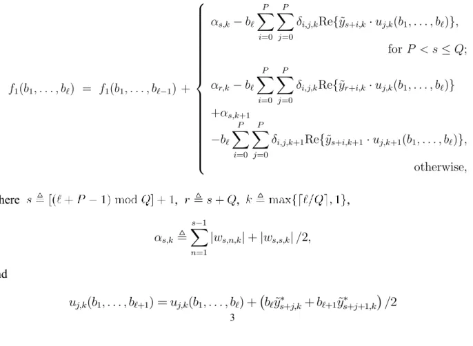
and is the (i,j)-th entry of matrix . By adding a constant to the decoding criterion, the on-the-fly metric that suits for the recursive computation of the priority-first search is given by:
f1(b1; : : : ; b`) = f1(b1; : : : ; b`¡1) + 8 > > > > > > > > > > > > > > > > > < > > > > > > > > > > > > > > > > > : ®s;k¡ b` P X i=0 P X j=0
±i;j;kRef~ys+i;k¢ uj;k(b1; : : : ; b`)g;
for P < s · Q; ®r;k¡ b` P X i=0 P X j=0
±i;j;kRef~yr+i;k ¢ uj;k(b1; : : : ; b`)g
+®s;k+1 ¡b` P X i=0 P X j=0
±i;j;k+1Ref~ys+i;k+1¢ uj;k+1(b1; : : : ; b`)g;
otherwise, where , , , ®s;k , s¡1 X n=1 jws;n;kj + jws;s;kj =2; and uj;k(b1; : : : ; b`+1) = uj;k(b1; : : : ; b`) + ¡ b`y~¤s+j;k+ b`+1y~¤s+j+1;k ¢ =2
with initial values for , and for and . The low-complexity decoding metric is given by
f2(b1; : : : ; b`) = f1(b1; : : : ; b`) + h(b1; : : : ; b`); where h(b1; : : : ; b`) , 8 > > > > > > > > > > > > > > > < > > > > > > > > > > > > > > > : Q+PX m=s+1 ®m;k¡ Q+PX m=s+1 jvm;k(b1; : : : ; b`)j ¡ ¯s;k for P < s · Q; Q+PX m=s+1 ®m;k+1¡ Q+PX m=s+1 jvm;k+1(b1; : : : ; b`)j ¡ ¯s;k+1 + Q+PX m=r+1 ®m;k ¡ Q+PX m=r+1 jvm;k(b1; : : : ; b`)j ¡ ¯r;k otherwise; where s, r and k are defined the same as for ,
vm;k(b1; : : : ; b`) = vm;k(b1; : : : ; b`¡1) + ws;m;kb`; and ¯s;k = ¯s¡1;k¡ Q+PX n=s+1 jws;n;kj ¡ 1 2jws;s;kj
with initial values and .
2.1.4 Achievement:
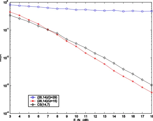
The channel parameters in simulations is zero-mean complex-Gaussian distributed with . Note again that is assumed an unknown constant vector at the system design stage; hence, the system designer does not know whether is zero-mean complex-Gaussian distributed. Figure 2 then simulates three half-rate codes over frequency selective channels of memory order 1, in which the channel coefficients vary independently in every 15 symbols. The three codes are identified by (28, 14)(Q = 29)(Q = 29), (28, 14)(Q = 15)(Q = 15) and CS(14, 7), which respectively represent the constructed (28, 14) code with design parameter Q = 29
Q = 29 (i.e., assuming at the design stage, the channel coefficients remain constant at least during the entire decoding block L = N + P = 28 + 1 = 29L = N + P = 28 + 1 = 29), the constructed (28, 14) code with
design parameter Q = 15Q = 15 (i.e., assuming the channel coefficients vary in every 15 symbols at the design stage), and the computer-searched (hence, structureless) (14, 7) code that minimizes the union bound derived based on the assumption that the channel taps remain constant during the decoding block (i.e., Q = L = N + P = 14 + 1 = 15Q = L = N + P = 14 + 1 = 15, which is exactly the simulated channel).
5
Figure 2: Word error rates (WERs) for the (28, 14)(Q=29) code, the (28, 14)(Q=15) code and the CS(14, 7) code over channels of memory order 1, whose coefficients varying independently in every 15 symbols.
As anticipated, (28, 14)(Q = 29)(Q = 29) code seriously degrades in performance since its
corresponding assumption at the design stage does not match the characteristic of the true simulated channel. This suggests that the assumption that the channel coefficients remain constant in a coding block is very critical in the code design, and should be made with caution. A striking result from Figure 2 is that the constructed (28, 14)(Q = 15)(Q = 15) code performs markedly
better than the CS(14, 7) code at medium-to-high signal-to-noise ratios, despite that the CS(14, 7) code is the computer-optimized code specifically for the simulated channel. This suggests that when the channel memory order and varying characteristic are prior known (i.e., PP and QQ), performance gain can be obtained by enhancing the inter-Q-block correlation, and the system favors a longer code design. In Table 1, we summarize the decoding complexity for the (28, 14)
(Q = 15)
(Q = 15) code simulated in Figure 2, measured by the average number of node expansions per
information bit. It shows, as previously mentioned, that the decoding metric requires less decoding efforts than the on-the-fly decoding metric .
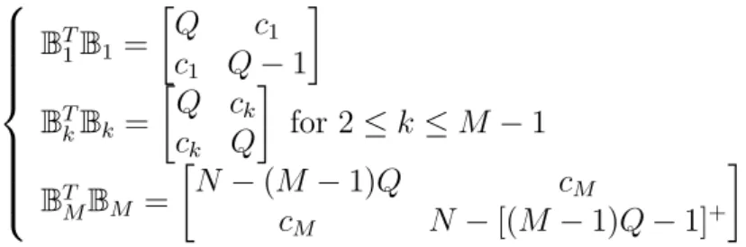
The performance of our constructed code can be further (slightly) improved if the codewords are selected uniformly from all feasible code design parameters . For example, select only half (i.e., ) of the codewords according to and for the (28, 14)(Q = 15)(Q = 15) code, and pick the remaining half of the codewords from those binary
8 > > > > > > < > > > > > > : BT 1B1 = · Q c1 c1 Q ¡ 1 ¸ BT kBk = · Q ck ck Q ¸ for 2 · k · M ¡ 1 BT MBM = · N ¡ (M ¡ 1)Q cM cM N ¡ [(M ¡ 1)Q ¡ 1]+ ¸
with and . This however will slightly increase the decoding complexity. The trade-off between selecting codewords from fixed or multiple 's is thus evident.
SNR 3dB 4dB 5dB 6dB 7dB 8dB 9dB 10dB 11dB 12dB 13dB 14dB 15dB 1658 1367 1074 899 701 593 488 448 356 309 277 244 232 766 625 482 392 321 254 219 177 149 133 121 104 92 / 2.2 2.2 2.2 2.3 2.2 2.3 2.5 2.4 2.4 2.3 2.3 2.3 2.5
Table 1: Average number of node expansions per information bit for the (28, 14)(Q=15) code simulated in Figure 1.
2.2 Reviews of the work in the second year:
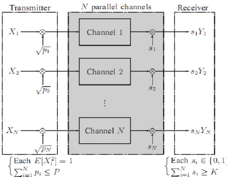
As the number of mobile users as well as the requirement for data rate is rapidly increasing in modern communication systems, the base stations are gradually evolved from macro-cell-based to micro-cell-based. In particular, the service range of a macro-cell base station may be partitioned into several small ones, which are in turn served by several micro-cell base stations[4]. As such, in order to maintain the seamless data transmission, signals from multiple base stations are required to provide softer handover functionality. On the other hand, the demand for mobility is also increased recently, resulting in a more frequent softer handover. Thus, in order to provide high mobility and high data transmission rate simultaneously, we consider in this project a novel system, in which the data is encoded and distributed over N base stations such that the receiver can decode data successfully as long as a certain portion of signals (at least K) from N base stations are received. Since the channel model only requires at least K among N signals are received, it is named the (N,K)-limited access channel. In the second year of this project, we analyzed the channel capacity of (N,K)-limited access channel with arbitrary channel models and proposed an fast algorithm to evaluate the optimal power allocation which achieves the channel capacity.
2.2.1 The system model:
7
only a certain portion of channel outputs are guaranteed to be successfully received at the receiver end. The receiver however does not a priori know which outputs will be nullified or blocked, nor does the receiver have the knowledge of the statistics of these blockages. We can realize this assumption by introducing a set of auxiliary multiplicative constants s1; s2; : : : ; sN
to the channel outputs, where the ith channel output is nullified when being multiplied by si = 0,
and remains when the multiplicative constant si is equal to 1. It is assumed that by monitoring
the channel activities, the receiver can perfectly tell the value of s = [s1; s2; : : : ; sN]T:
Furthermore, s will remain constant within a codeword transmission period but may vary for different codeword blocks. The receiver will then decode the information based on the receptions
[s ± Y1; s ± Y2; : : : ; s ± Yn] if at least K out of N components of vector s are equal to one,
where Yi, [Y1;i; Y2;i; : : : ; YN;i]T are the channel symbols received at time instance i, n is the
codeword length, and operator \ ± " denotes the matrix Hadamard product[5]. Conversely, the
receiver will give up the decoding if PN
i=1si< K. We thus refer to this channel model as an
(N,K)-limited access channel.
In this setting, we are interested in the optimal power allocation p¤= [p¤
1; p¤2; : : : ; p¤N]T such
that the minimum input-output mutual information subject to PN
i=1si¸ K is maximized. This
quantity is generally regarded as the achievable rate under which the decoding error can be made arbitrarily small.
Figure 3: System model for an (N; K)-limited access channel.
Under the system model, the input-output mutual information can be in principle represented by
where I(¢; ¢) is the mutual information function and pp , [pp1;
p
p2; : : : ;
p
pN]T. Here, we
overload the notation by denoting the channel output vector corresponding to one channel usage by Y = [Y1; Y2; : : : ; YN]T, and likewisely denote by X = [X1; X2; : : : ; XN]T the channel input
vector for a single channel usage. The achievable rate that guarantees a vanishing decoding error subject to PN
i=1si¸ K is therefore optimistically
max max f 2<N +: N i=1pi·P min f 2f0;1gN: N i=1si¸Kg I(pp ± X; s ± Y ) (2)
Where <+ is the set of nonnegative real numbers. If the parallel channels are independent in the
sense that Pr(Y jpp ± X) = N Y i=1 Pr(Yij p piXi) (3)
then the independence bound for mutual information gives that I(pp ± X; s ± Y ) · N X i=1 I(ppiXi; siYi) = N X i=1 siI( p piXi; Yi)
where the last equality follows from that si is either 1 or 0. We can therefore focus on the
optimal power allocation for independent input distributions, if the channel transition probability satisfies (3).
We next denote for convenience fi(p) , I(
p
piXi; Yi) for 1 · i · N, and make the
following assumption on these mutual information functions.
Assumption 1: For 1 · i · N; fi(p) is continuous and strictly increasing for p ¸ 0, and its first
derivative, i.e.,
fi0(p) , @fi(p) @p
exists and is continuous and strictly decreasing in p ¸ 0, where we define f0
i(0) , limp#0fi0(p).
This assumption will be adopted as a premise in the following analysis. Under Assumption 1, it is clear that fi(p) is a strictly concave function of p with initial value fi(0) = I(0; Yi) = 0.
Together with the fact that fi(p) ¸ 0 for p 2 <+, we can replace the two inequality constraints
in (2) by their equality counterparts as
max f 2<N +: Ni=1pi·P min f 2f0;1gN: N i=1si¸Kg PN i=1si¢ fi(pi) = max f 2<N +: Ni=1pi=P min f 2f0;1gN: N i=1si=Kg PN i=1si¢ fi(pi) (4)
for a given that validates Assumption 1.
9
problem in (3) becomes algorithmically tractable (cf. Theorem 2). 2.2.2 Analysis of The optimal power allocation
In this section, the analysis for the optimization problem in (4) is presented. For 𝐾 = 1, (4) can be simplified to
max f 2<N +: N i=1pi=Pg minff1(p1); f2(p2); : : : ; fN(PN)g:
It is thus straightforward that the optimal power allocation p¤ satisfies
f1(p¤1) = f2(p¤2) = ¢ ¢ ¢ = fN(p¤N)
For K = N, the maximization-minimization power allocation problem reduces to one that only requires a maximization computation because s1 = s2 = : : : = sN = 1. Therefore, one can
apply the Lagrange multipliers technique and Karush-Kuhn-Tucker (KKT) condition to find the optimal power allocation [6]. However, for 1 < K < N, there does not exist a straight technique for this maximization-minimization problem. Nevertheless, we can find a necessary condition for the optimal power allocation such that the labor of examining all possible ¡N
K
¢
combinations of s satisfying PNi=1si¸ K can be reduced as indicated in the next lemma.
Lemma 1: The optimal power allocation p¤ for an (N,K)-limited access channel satisfies
fa1(p ¤ a1) · fa2(p ¤ a2) · ¢ ¢ ¢ · faK(p ¤ aK) = faK+1(p ¤ aK+1) = ¢ ¢ ¢ = faN(p ¤ aN)
for some permutation a1; a2; : : : ; aN of sequence 1; 2; : : : ; N.
An immediate implication of Lemma 1 is that we can distinguish the optimal power allocation for an (N,K)-limited access channel into K disjoint cases. In other words, the condition
max 1·i·`¡1fai(p ¤ ai) < fa`(p ¤ a`) = fa`+1(p ¤ a`+1) = ¢ ¢ ¢ = faN(p ¤ aN) (5)
is valid exactly for one value of ` in f1; 2; : : : ; Kg. As a result, if the index set
A , fa`; a`+1; ¢ ¢ ¢ ; aNg
in which their respective mutual information function values are equal to max1·i·Nfi(p¤i) is
identified in advance, the maximization-minimization power allocation problem is simplified to a maximization problem as max 2P(A) ( X i =2A fi(pi) + (K ¡ N + jAj) max 1·j·Nfj(pj) ) (6) where
P(A) , 8 < :p 2 < N + : (i)PNi=1pi= P
(ii)fi(pi) < max1·j·Nfj(pj) for i =2 A
(iii)fi(pi) = max1·j·Nfj(pj) for i 2 A
9 =
;: (7)
However, the direct identification of A without knowing p¤ in advance is in general a
challenged. The opposite, i.e., identifying A after determining p¤, is more straightforward. In
order to resolve the optimization problem, we propose in the following subsections to first determine the best power allocation p¦ corresponding to a conjectured
maximal-mutual-information index set, denoted by B. Then, we will examine afterwards whether this conjecture is the optimal one or not based on some condition we will establish later. In case the conjectured B only achieves a suboptimal power allocation, a new round of maximization computation and follow-up examination will be launched based on a newly generated B. Since the established condition will help identifying one index that is not in A at each round, the
process can hopefully stop after N ¡ jAj + 1 iterations after which p¤ is obtained.
A. Determination of the best power allocation p¦ corresponding to a given index set B
Based on a given index set B, we transform the maximization-minimization problem into sup
2P(B)
f Pi =2Bfi(pi) + (K ¡ N + jBj) max1·j·Nfj(pj)g (8)
where P (B) is defined the same as (7) except that A is replaced with B. Since the given B
may not be the optimal index set A, the solution p¦ of the optimization problem defined in (8)
could be at the boundary of P (B) in the sense that
fi(p¦i) = max1·j·Nfj(p¦j) for some i =2 B:
For this reason, we use supremum instead of maximum in (8).
We next show that this inequality constraint can be relaxed by means of the incorporation of the aggregate mutual information function that transforms the N-dimensional power allocation problem into an equivalent N ¡ jBj + 1-dimensional one.
Definition 1: The aggregate mutual information function FB with respect to a sequence of
mutual information functions ffigi2B is defined through its inverse function as
FB(inv)(y) ,X
i2B
fi(inv)(y) for y ¸ 0 (9)
11
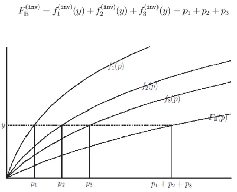
A graphical illustration of the aggregate mutual information function for B = f1; 2; 3g is given in Figure 4. In this figure, it is clear that
FB(inv)= f1(inv)(y) + f2(inv)(y) + f3(inv)(y) = p1+ p2+ p3
Figure 4: Graphical illustration of the aggregate mutual information function when fi(p) = log(1 + p=¾2i) and ¾2i = i for i 2 B = f1; 2; 3g.
As a specific example, if fi(p) = log(1 + p=¾i2) for some ¾2i > 0 and 1 · i · 3, then
FB(p) = log µ 1 + p ¾2 1+ ¾22+ ¾32 ¶ :
In terms of the aggregate mutual information function, we can simplify the constraints in P (B)
in the following lemma.
Lemma 2: Fix an index set B. The solution p¦ of the optimization problem in (8) satisfies
p¦i = ( q¦ i for i =2 B fi(inv)(FB(q¦B)) for i 2 B (10) where the N ¡ jBj + 1-dimensional vector q¦ is the solution of the optimization problem
below: sup 2Q(B) f Pi =2Bfi(qi) + (K ¡ N + jBj)FB(qB)g (11) where Q(B) , ½ q = (list of qi8i =2 B; qB) 2 < N¡jBj+1 + : (i)Pi =2Bqi+ qB = P (ii)fi(qi) < FB(qB) for i =2 B ¾ :
By the reduction of constraints down to two in Q(B) in Lemma 2, we can further proceed to show that the inequality constraint in Q(B) is redundant in case q¦ 2 Q(B) as summarized in Theorem 1.
Theorem 1: Given that q¦ 2 Q(B), the maximize q¦ for (11) is equal to the maximize ~q of the
problem below: max 2 ~Q(B) fPi =2Bfi(qi) + (K ¡ N + jBj)FB(qB)g (12) where ~ Q(B) , fq 2 <N¡jBj+1+ : P i=2Bqi+ qB= Pg
We conclude this subsection by pointing out that the maximization computation in (12) is now performed over the usual single power-sum constraint, and hence can be solved by the Lagrange multipliers technique and KKT condition by treating (K ¡ N + jBj)FB(qB) as the
mutual information function of an auxiliary aggregate channel. Based on the result in Theorem 1, we are ready to present the algorithmic approach that helps identifying the optimal maximal-mutual-information index set A and the optimal power allocation p¤.
B. Determination of the Optimal Maximal-Mutual-Information Index Set 𝔸 and the Optimal Power Allocation 𝒑∗
For an (N,K)-limited access channel, there are possibly PK `=1
¡N
`¡1
¢
candidate index sets for the choices of B in Theorem 1, and it may be time-consuming to perform the optimization computation for (12) for each of them. The next theorem then shows that this time-consuming maximization labor can be reduced to only N ¡ jAj + 1.
Theorem 2: The optimal maximal-mutual-information index set A as well as the optimal power
allocation p¤ can be obtained through the following algorithmic procedure:
Step 1. Initialize M = 1 and B1 = f1; 2; : : : ; N g.
Step 2. Obtain the maximize q~M for (12) by setting B = BM, and calculate
~
pM = [~pM;1; ~pM;2; ¢ ¢ ¢ ; ~pM;N]T
corresponding to the obtained q~M and the given BM through an assignment similar to (10).
Step 3. Assign BM +1 = BM n fjMg where jM is an index in BM that satisfies
fj0M(~pM;jM) = min
i2BM
fi0(~pM;i) (13)
(If there are more than one indices satisfying (13), just pick up any one of them as jM.)
13
(K ¡ M)FB0M+1(Pi2B
M+1p~M;i) · f
0
jM(~pM;jM) (14)
then set A = BM and p¤= ~pM and stop the algorithm; otherwise, set M = M + 1 and go
to Step 2.
We would like to point out that the algorithm in Theorem 2 will stop when (usually before) M reaches K because (14) trivially holds when M = K. This coincides with the definition of
A in (5) that at most K ¡ 1 indices are outside A.
Theorem 2 indicates that given the first derivative of the marginal mutual information
function fi(p) = I(
p
pXi; Yi) being positive, strictly decreasing and continuous in p for every
1 · i · N (i.e., Assumption 1), we can determine the optimal power allocation p¤ for a spatially
independent (N,K)-limited access channel with input pp ± X by performing N ¡ jAj + 1
maximizations in the sense of (12). 2.2.3 Achievement:
For (N; K )-limited access channels with arbitrary inputs, the capacity formula is derived as a
maximization-minimization problem. We then analyze the maximization-minimization problem to get two properties as shown in Lemma 1 and Lemma 2. According to these two properties and the definition of aggregate mutual information, we then simplify the maximization-minimization problem to a simple maximization problem with only one single power-sum constraint. Based on the simple maximization problem with single power-sum constraint, we propose an algorithm to find the optimal power allocation p¤ by N ¡ jAj + 1 time-consuming maximization labor. 3. 報告內容(第三年)
3.1 Introduction:
In the second year of this project, we have proposed an algorithm of finding the optimal power allocation for general channels with limited access constraint. Following the proposed algorithm, in this year we further establish that when channel disturbances, in addition to independence, are reduced to being additive with distributions scaled from a common random variable, the optimal power allocation can be directly obtained from a two-phase water-filling process if the arbitrary inputs are given by the respective component variables in an independent and identical distributed (i.i.d.) random vector, multiplying by the square root of the allocated power. The two-phase water-filling interpretation then hints that the degree of “noisiness” for a general (possibly, non-additive and non-Gaussian) limited access channel might be identified by composing the derivative of the mutual information function with its inverse.
3.2 The system model:
Although Gaussians are generally appropriate noise models for physical additive channels, experimental measurement indicates that the noises in certain environments are by no means Gaussian distributed [7][8][9]. As such, in the third year of this project, we consider additive noise of the same family in (N; K )-limited access channels.
By additive noises of the same family, we mean that the relationship between channel inputs and outputs can be characterized by
Yi=
p
piXi+ ¾iZi for 1 · i · N (15)
where fXigNi=1 and fZigNi=1 are both i.i.d. complex random variables with unit second moments,
and they are independent from each other; the system model is shown as Figure 5.
Figure 5: System model for an (N; K)-limited access channel with additive noise of the same family, where E[jXij2] = E[jZij2] = 1, si2 f0; 1g for 1 · i · N ,
PN
i=1si¸ K and
PN
i=1pi· P.
We then restrict our attention only to the case that Zi is a continuous random variable
because Assumption 1(at page 8) may fail when both Xi and Zi are discrete. Notably, Xi often
takes values in a finite alphabet (e.g., f§1g) in practice. Specifically, when the intersection of
two sets ©ppix + ¾iz : PZi(z) > 0
ª
and ©ppix + ¾~ iz : PZi(z) > 0
ª
is empty for every x 6= ~x with PXi(x) > 0 and PXi(~x) > 0, we have
fi(pi) = I(
p
piXi; Yi) = H(
p
piXi) = H(Xi)
where H(Xi) is the entropy of the channel input Xi [10]. This implies that in a discrete system,
fi(pi) can be equal to its maximum value H(Xi) almost everywhere in pi, in which case
Assumption 1 is unquestionably violated.
15 I(ppiXi; Yi) = h(Yi) ¡ h(Yij p piXi) = h(Yi) ¡ h( p piXi+ ¾iZij p piXi) = h(¾iY~i) ¡ h(¾iZi) (16) = h( ~Yi) ¡ h(Zi) = I µp pi ¾i Xi; ~Yi ¶
where h(¢) is the differential entropy function [10], and (16) follows from the independence between Xi andZi, and ~Yi, (
p
pi=¾i)Xi+ Zi. This immediately yields
fi(pi) = g µ pi ¾2 i ¶ for every 1 · i · N (17) with g(½) , I(p½Xi; p ½Xi+ Zi): (18)
Assumption 1 thus reduces to the single condition that function g is continuous and strictly
increasing, and its first derivative exists and is continuous and strictly decreasing. 3.3 The optimal power allocation for additive noise of the same family:
Based on this system setting, we show in the next theorem that the optimal power allocation p¤ follows a two-phase water-filling scheme} Specifically, in the first phase (which we refer to
as the noise-power re-distribution phase), the least N ¡ K noise powers among f¾2
igNi=1 will
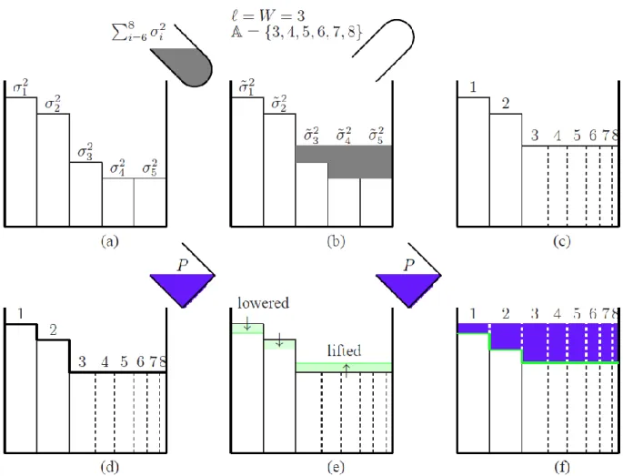
be first poured as noise water into a tank consisting of K interconnected vessels with solid base heights equal to the remaining K noise powers and with widths of unit length as shown in Figure 6(b). Afterwards those W vessels either with water inside or with solid base height equal to the water surface level will be subdivided into N ¡ K + W vessels of rectangular shape with
the same heights (as the water surface level) and with widths in proportion to their noise powers (but the total volume remaining unchanged). As such, a tank with N vessels of proper heights and widths (corresponding to N channels) is ready for the second phase as exemplified in Figure 6(c). It is worth mentioning that after the first phase, the optimal maximal-mutual-information index set A has already been identified and consists of the channel
indices corresponding to the aforementioned W vessels and the least N ¡ K noise powers (hence, jAj = W + N ¡ K).
In the second phase (which we refer to as the signal-power allocation phase), the heights of vessel bases will be first either lifted or possibly lowered according to total signal power P and function g as well as their current heights as shown in Figure 6(e). What follows, as exemplified in Figure 6(f), is the usual water-filling power allocation scheme. The pre-adjustment of base heights before water filling can be viewed as preparation for these vessels to be “capable” of
supporting the water that is going to be poured in with amount P. As a result, the volume of water ended up in each vessel is exactly the power that should be allocated. Notably, for the special case that the noises fZigNi=1 are complex Gaussian distributed, the heights of vessel bases
can never be lowered in the pre-adjustment step; hence, a mercury-filling scheme before water pouring has been proposed to materialize the lifting of heights of vessel bases [11]. However, since the adjustment of heights of vessel bases generally can be in both up and down directions, the use of the name mercury/water filling may induce that the vessel bases should be lifted under general non-Gaussian additive noises; hence, we simply use the conventional name of water-filling in this work.
Theorem 3: Suppose that the information transmitted over an (N; K )-limited access channel is
corrupted by additive noises of the same family characterized by (15) and the mutual information function g(½) defined in (18) satisfies Assumption 1. Assume without loss of generality that
¾21 ¸ ¾22¸ ¢ ¢ ¢ ¸ ¾N2:
Then, the optimal maximal-mutual-information index set A is given by
A = f`; ` + 1; ¢ ¢ ¢ ; N g (19) where ` , min ½ i 2 f1; 2; ¢ ¢ ¢ ; Kg ¯ ¯ ¯ ¯¾2i · ~¾ 2 K for every 1 · i · K ¾ (20) and ~¾2
i , ¾2i + [¸ ¡ ¾2i]+ for 1 · i · K with ¸ chosen to satisfy
PK
i=1[¸ ¡ ¾i2] +
=PNi=K+1¾2
i, and [y]+, maxf0; yg. The optimal power allocation p¤ can
therefore be obtained from q¤ through an assignment similar to (10), where q¤ is the maximizer
for (12) with B equal to the above A. In other words, p¤i = ( q¤ i for 1 · i < ` ¾2 i N j=`¾j2 ¢ q¤ A for ` · i · N (21) with qi¤= ½ ¾2 i ¢ g0(inv) ¡ º ¾2 i ¢ if g0(1) < º¾2 i < g0(0) 0 if º¾2 i ¸ g0(0) ¾ for 1 · i < ` (22) and qA¤ = à N X j=` ¾2j ! ¢ g0(inv) à º PN j=`¾j2 K ¡ ` + 1 ! (23) where g0(inv) is the inverse function of the first derivative g0 of function g, and º is chosen
17
P`¡1
i=1q ¤
i + qA¤ = P: (24)
Figure 6: The graphical interpretation of the optimal two-phase water-filling power allocation for an (8; 5)
-limited access channel with independent additive noises characterized by (15). In this figure, [¾2
1; ¾22; ¢ ¢ ¢ ; ¾82] = [8; 7; 4; 3; 3; 2; 2; 1]. Subfigures (a), (b) and (c) correspond to the noise-power redistribution phase,
while subfigures (d), (e) and (f) illustrate the signal-power allocation phase.
Several remarks can be made based on Theorem 3.
First, it can be extended from Theorem 3 that as long as A is pre-determined, the
maximization labor can always be reduced down to one. In the special case that the noises are additive and originated from the same family (as considered in this section), we can directly determine A in terms of (20).
Secondly, when ` = 1 (equivalently, A = f1; 2; : : : ; N g), p¤ can be determined without
any maximization labor since we immediately have q¤
A = P by (24). In such a case, the
optimal power allocation follows the equal signal-to-noise ratio (SNR) principle as
p¤ i ¾2 i = PNP j=1¾2j for every 1 · i · N:
Finally, the validity of Theorem 3 does not need to be restricted to channels with additive noises of the same family but can be extended to any (N; K )-limited access channel with marginal mutual information functions satisfying (17) for some function g that obeys
Assumption 1. A straightforward example is the flat fading channels with known channel
states at the receiver end, characterized by
Yi = (¯iHi)(
p
piXi) + ¾iZi for 1 · i · N (25)
where fHigNi=1 is i.i.d. with unit second moment, and is independent of the channel input
and additive noise. We then obtain fi(pi) = g(¯i2pi=¾i2) with
g(½) = I(p½Xi;
p
½HiXi+ ZijHi). Theorem 3 thus can be used to establish the optimal
power allocation by treating ¾2
i=¯i2 as the new noise power level.
An exemplified illustration of the two-phase water-filling scheme is depicted in Figure 6. Details are given below.
<The noise-power re-distribution phase>
Fig. 6(a) Set K vessels with widths of unit length and with base height of the ith vessel being ¾2
i for 1 · i · K. (Note that we assume ¾12¸ ¾22¸ ¢ ¢ ¢ ¸ ¾N2.)
Fig. 6(b) Pour in the “noise water” of amount PN
j=K+1¾j2 and set ¾~2i as the new water level of
vessel i for 1 · i · K. Let ` be the smallest integer among f1; 2; : : : ; Kg such that ¾2
i · ~¾K2 (cf. (20)). Assign A = f`; ` + 1; : : : ; N g and W = K ¡ ` + 1.
Fig. 6(c) Sub-divide the space of the last W vessels (i.e., K ¡ W + 1; K ¡ W + 2; : : : ; K)
into W + (N ¡ K) new vessels of rectangular shape with base height the same as the water surface level and widths in proportion to ¾2
i for ` · i · N. < The signal-power allocation phase >
Fig. 6(d) Retain the N vessels from the previous phase. Fig. 6(e) Adjust the base height of the ith vessel to
Li(º) , ( ¾2 i ¢ G(º¾i2) for 1 · i < ` ~ ¾2 K¢ G(º ~¾2K) for ` · i · N (26) where º is the parameter chosen in Theorem 3 according to (24), and
G(³) , ( 1 ³ ¡ g 0(inv)(³) if g0(1) < ³ < g0(0) 1 g0(0) if ³ ¸ g 0(0):
Fig. 6(f) Pour in the “signal water” of amount P. Then the volume of water in the ith vessel is
the optimal power p¤
i to be allocated for channel i.
3.4 Implications from the optimal power allocation:
Theorem 2 indicates that the sequence of candidate maximal-mutual-information index sets
19
can be regarded as sorting the channels in their descending degrees of “noisiness,” which can be supported by the result from Theorem 3, where the sequence of j1; j2; j3; : : : coincides with
¾2 j1 ¸ ¾ 2 j2 ¸ ¾ 2 j3 ¸ ¢ ¢ ¢ :
For a general (N; K )-limited access channel in which the noises are not necessarily additive or scaled from the same family, can one identify such sequence through their mutual information functions? The next theorem may provide a guide along this direction of thinking.
Theorem 4: For a general (N; K )-limited access channel, if fk01 ³ fk(inv)1 (y) ´ · fk02 ³ fk(inv)2 (y) ´ · ¢ ¢ ¢ · fk0N ³ fk(inv)N (y) ´ for all y ¸ 0 then jM= kM for M = 1; 2; 3; : : :.
Here, regardless of the original goal of the determination of optimal power allocation,
Theorem 4 (as an extension from Theorem 3) proposes a way to compare the degree of “noisiness”
of general channels via their mutual information functions. For the additive noise channels of the same family, we have
fi0 ³ fi(inv)(y) ´ = 1 ¾2 i g0¡g(inv)(y)¢:
Hence, the proposed ordering coincides with the general impression that the larger the ¾2 i, the
noisier the ith channel is considered to be. To simplify the notation, we drop the parentheses
between f0
i and f
(inv)
i in the sequel.
For channels other than additive noise of the same family, there could be no apparent winner between any two channels in the sense of ff0
if (inv)
i gNi=1. In other words, it could happen that
fi0fi(inv)(y1) > fj0f (inv) j (y1) but fi0f (inv) i (y2) < fj0f (inv) j (y2)
for two distinct y1 and y2 and two distinct i and j. As such, the sequence of j1; j2; j3; : : : will
become a function of the total signal power P. However, if a certain condition is satisfied, the pre-identification of the degrees of channel noisiness is still possible at two extreme situations: P ! 0 and P ! 1, which we will respectively refer to as the low- and high-power regimes in later discussion. Lemma 3: 1. If lim sup y#0 ³
fi0fi(inv)(y) ¡ fj0fj(inv)(y) ´
· 0 for every 1 · i < j · N (27) then ji = i in the low-power regime, where sign function sgn(½) is equal to either 1,
2. If lim sup y"minf!i;!jg sgn ³ fi0f (inv) i (y) ¡ f 0 jf (inv) j (y) ´ · 0 for every 1 · i < j · N (28)
then ji = i in the high-power regime, provided that limp!1fi0(p) = 0 for 1 · i · N,
where !i, limp!1fi(p).
Since the input alphabet is usually finite for channels of practical interest, we have
!i, limp!1fi(p) · H(Xi) < 1: This immediately validates the premise, i.e.,
limp!1fi0(p) = 0, for condition (28) implying ji = i in the high-power regime. In other
words, limp!1fi0(p) = 0 is true for all finite-input channels. There however exists a certain
kind of channels where !i= 1 while limp!1fi0(p) = 0. An example is the Gaussian-input
AWGN channel for which fi(p) = log (1 + p=¾2i). We would like to emphasize that the inference
regarding (28) still remains valid for channels with unbounded mutual information as long as
limp!1fi0(p) = 0.
Conditions (27) and (28) in Lemma 3 involve the examination of the limit supremum of function differences. The following corollary shows that their validity can be guaranteed by comparing the limiting behaviors of individual functions.
Corollary 1:
1. The validity of (27) for an (i; j) pair is certain if one of the three conditions below is satisfied: 8 > < > : f0 i(0) < fj0(0) f0 i(0) = fj0(0) and f ( i0) < f ( j0) (9 ± > 0) f0 i(p) · fj0(p) for 0 < p < ± (29) 2. The validity of (28) for an (i; j) pair is certain if
!i = lim
p!1fi(p) < !j = limp!1fj(p): (30)
According to the above discussions, we can identify the degree of noisiness for general channel easily by the sufficient conditions provided in Theorem 4, Lemma 3 and Corollary 1. 4. Reference
[1] Y. S. Han and P.-N. Chen, “Sequential decoding of convolutional codes,” The Wiley
Encyclopedia of Telecommunications, edited J. Proakis, John Wiley and Sons, Inc., 2002.
[2] Y. S. Han, C. R. P. Hartmann and C.-C. Chen, “Efficient priority-first search maximum-likelihood soft-decision decoding of linear block codes,” IEEE Trans. Inform.
Theory, vol. 39, no. 5, pp. 1514–1523, Sep. 1993.
21
[4] H. Holma and A. Toskala, WCDMA for UMTS: HSPA Evolution and LTE, 4th ed.. Chichester: UK, Wiley, 2007.
[5] R. A. Horn and C. R. Johnson, Matrix Analysis. Cambridge, U.K.: Cambridge Univ. Press, 1985.
[6] S. Boyd and L. Vandenberghe, Convex Optimization. Cambridge, U.K.: Cambridge Univ. Press, 2004.
[7] K. L. Blackard, T. S. Rappaport, and C. W. Bostain, “Measurements and models of radio frequency impulsive noise for indoor wireless communications,” IEEE J. Sel. Areas
Commun., vol. 11, no. 7, pp. 991-1001, Sep. 1993.
[8] M. G. Sanchez, A. V. Alejos, and I. Cuinas, “Urban wide-band measurements of the UMTS electromagnetic environment,” IEEE Trans. Veh. Technol., vol. 53, no. 4, pp. 1014-1022, Jul. 2004.
[9] M. Zimermann and K. Dostert, “Analysis and modeling of impulsive noise in broad-band powerline communications,” IEEE Trans. Electromagn. Compat., vol. 44, no. 1, pp. 249-258, Feb. 2002.
[10] T. M. Cover and J. A. Thomas, Elements of Information Theory. New York: Wiley, 1991. [11] A. Lozano, A. M. Tulino, and S. Verdu, “Optimal power allocation for parallel Gaussian
channels with arbitrary input distributions,” IEEE Trans. Inf. Theory, vol. 52, no. 7, pp. 3033-3051, Jul. 2006.
4. 計畫成果自評
In this three-years project, we have investigated several scenarios of codes designing for non-coherent detection system that combines channel estimation and error correction. This design can directly construct a code of any desired code length and code rate, of which the performance is shown to be comparable to the best computer-searched code for the channels simulated. For the designing and analysis of the novel (N; K )-limited access system, we have derived the channel capacity and proposed a fast algorithm of finding optimal power allocation to achieve the capacity. Following the proposed algorithm, the optimal power allocation can be obtained by a two-phase water-filling process when the channel model is additive noise of the same family. From the interpretation of two-phase water-filling, we further define the degree of noisiness for general channels. The works for the novel (N; K )-limited access system will appear in IEEE
Transactions on Information Theory and was presented in part at the 2011 International Symposium on Information Theory.
![Figure 5: System model for an (N; K) -limited access channel with additive noise of the same family, where E[jX i j 2 ] = E[jZ i j 2 ] = 1, s i 2 f0; 1g for 1 · i · N , P N i=1 s i ¸ K and P N i=1 p i · P .](https://thumb-ap.123doks.com/thumbv2/9libinfo/8214940.170235/16.892.248.680.436.721/figure-model-limited-access-channel-additive-noise-family.webp)