考慮韋伯製程平均發生偏移下之製程能力調整

全文

(1)國立交通大學工業工程與管理學系碩士班. 碩士論文. 考慮韋伯製程平均發生偏移下之製程能力調整 Capability Adjustment for Weibull Processes with Mean Shift Consideration. 研究生：盧俊昇指導教授：彭文理博士. 中華民國九十七年七月.

(2) 考慮韋伯製程平均發生偏移下之製程能力調整. Capability Adjustment for Weibull Processes with Mean Shift Consideration Student：Chun-Seng Lu Advisor：Dr. W. L. Pearn. 研究生：盧俊昇指導教授：彭文理博士. 國立交通大學工業工程與管理學系碩士論文. A Thesis Submitted to Department of Industrial Engineering and Management College of Management National Chiao Tung University in partial Fulfillment of the Requirements for the Degree of Master in Industrial Engineering July 2008 Hsinchu, Taiwan, Republic of China. 中華民國九十七年七月.

(3) 考慮韋伯製程平均發生偏移下之製程能力調整研究生：盧俊昇. 指導教授：彭文理. 國立交通大學工業工程與管理學系碩士班. 摘要製程能力指標被用來衡量製程製造產品符合規格的能力，不僅是提供品質保證的工具，也是在品質改善方面的一個方針。計算製程能力指標需服從製程為穩態的前提假設，也就是在生產過程中平均數和標準差不會改變，但是在實務上製程為動態。當製程發生平均數微小偏移時，有些管制圖可能無法偵測到，造成製程能力指標高估製程良率，因此必須將製程能力指標進行調整。Bothe (2002) 提出製程服從常態分配下之製程能力調整方法。事實上，非常態分配製程在業界也時常出現，因此本研究將針對製程服從韋伯分配提出其製程能力調整方法。由於調整量的大小與管制圖檢定力息息相關，故本研究先比較三種不同的韋伯管制圖在相同平均偏移量下之檢定力。再選定檢定力最高的管制圖計算在韋伯分配下應調整的偏移量，並針對非常態適用的 C pk 指標做調整。在本研究的最後，我們用一個實例來說明如何在製程服從韋伯分配並考慮製程平均會發生變動，如何調整製程能力指標 C pk 。關鍵字：韋伯分配、韋伯管制圖、製程偏移、製程能力指標.

(4) Capability Adjustment for Weibull Processes with Mean Shift Consideration. Student: Chun Seng Lu. Advisor: Dr. W. L. Pearn. Department of Industrial Engineering and Management National Chiao Tung University Abstract Process capability indices (PCIs) have been proposed in the manufacturing industry to provide numerical measures on process reproduction capability, which are effective tools for quality assurance and guidance for process improvement. PCIs are calculated under the assumption that the process is stable (the process mean and variation are not change), but in practice, the process is dynamic. If the process mean has a small shift, the control chart doesn’t detect obviously so that the PCIs will overestimate the true process capability. For this reason, the PCIs have to be adjusted. Bothe (2002) provided the adjustment method for normality processes. In this paper, we provide capability adjustment method for Weibull processes. The magnitudes of adjustment is correlated with the detection power of control chart, so we first compare the detection powers of three Weibull control chart under the same mean shift distances, and choose the best powerful Weibull control chart to calculate the mean shift adjustments for Weibull processes. At the end, we add the adjustment to capability index C pk of non-normal processes. For illustration purpose, an application example is presented. Keywords: Dynamic C pk , Mean shift, Process capability index, Weibull distribution, Weibull control chart..

(5) 誌謝兩年的時間，說長不長，說短也不短，在這兩年的時光我完成了我畢生第一篇也可能是最後一篇論文。本人資質駑鈍，能完成它是經由許多貴人的幫助，首先我最要感謝的就是我的指導老師─彭文理博士，彭老師敎了我許多做學問以及做人應有的態度和方法，他的句句名言，相信會在我未來求職的路上帶來許多的助益。我也要感謝我口試的口試委員鍾淑馨老師、吳建瑋老師、徐雅甄老師在口試時明確指出我的缺失，讓我整篇論文能夠更加完整更有貢獻。新竹的生活相當苦悶，但是我有許多好朋友讓我在苦悶中獲得許多樂趣。感謝 MB517 的學長和同學爽斌、貝爾、佳煌、仲軒和秉爺時常為我解決一些論文或課業上我搞不懂的問題，也貢獻了許多食物，讓實驗室的糧食不虞匱乏。也感謝學弟妹品倫、律瑋、佳蕙、Poppy 帶給我在實驗室許多的歡樂，尤其是佳蕙和 Poppy 老是在我寫論文寫到很煩的時候都讓我欺負，讓我舒解了許多的壓力，感謝你們，祝你們能跟隨我的腳步順利畢業。我還要感謝 MB519 的垃圾同學小毛、苗人、迪喬、柏懿、小潔。519 實驗室是我的糧倉二號以及遊樂室，因為他們的零食總是比我們實驗室多，而且他們垃圾話永不間斷，讓我打發了許多無聊的時光。小毛雖然他很弱，但是他是我最好的電動戰友；苗人總是能講出許多垃圾話名言；迪喬灌籃高手和格鬥天王很強可是 NBA 很弱；柏懿創造許多讓我們打嘴砲的話題；小潔則是讓我們嗆的好對象。MB519 的大家，謝謝你們，因為有你們讓我研究所生活變的更有趣，更加有色彩。還有一些過去成大的好朋友及好戰友們，在新竹的臭雞、小吉、邱威、機巴瑞以及在台南的龜萱、娘達、廢物康、曾機巴、洋妞、阿坑、GB、好學弟娘豪，感謝妳們在我快樂的時候陪我快樂，在我失意的時候用很嚴厲的垃圾話安慰我，幫助我從難過中重新站起來，謝謝你們，有你們真好。最後我要特別感謝我的父母讓我在求學過程中有充足的資源能夠完全投入在念書中，不用去煩惱金錢的問題，對我也不會特別嚴厲，讓我在幸福的生活中成長。也感謝天父上帝時常保佑我，看顧我，讓我在人生中一路走來能順順利利，平平安安。我已完成了人生第一階段，將來還有更多挑戰在等著我，願我在研究所所學到的東西，能對我的將來帶來許多的幫助。最後，我想說，畢業好爽啊！. I.

(6) Contents Contents .......................................................................................................... II List of Tables ..................................................................................................III List of Figures ................................................................................................ IV 1. Introduction .................................................................................................. 1 1.1. Research Background and Motivation .....................................................1 1.2. Research Purpose and Objectives.............................................................2 1.3. Thesis Organization ................................................................................3 2. Literature Review .......................................................................................... 4 2.1. Process Capability Adjustment for Normal Processes...............................4 2.2. Process Capability Adjustment for Gamma Processes ..............................5 2.3. Process Capability Adjustment for Weibull Processes...............................7 3. Control Chart Power Analysis for Weibull Processes...................................... 9 3.1. The Weibull Processes.............................................................................9 3.2. The Detection Power of the Percentile Weibull Control Chart ................13 3.3. The Detection Power of the Bootstrap Weibull control chart ..................15 3.4. Erto’s Weibull Control Chart for Weibull Processes................................17 3.5. The Detection Power of Erto’s Weibull Control Chart ...........................19 3.6. Detection Power Comparisons ..............................................................21 4. Process Capability Adjustment for Weibull Processes ................................... 26 4.1 Estimator of C pk for Non-Normal Processes...........................................26 4.2 Process Capability Adjustment of C pk for Weibull Processes ...................26 5. An Application............................................................................................ 29 6. Conclusions ................................................................................................ 33 References ...................................................................................................... 34 Appendix A. Power Curve for Subgroup Size 4 and 6....................................... 36 Appendix B. Goodness-of-Fit Tests .................................................................. 40. II.

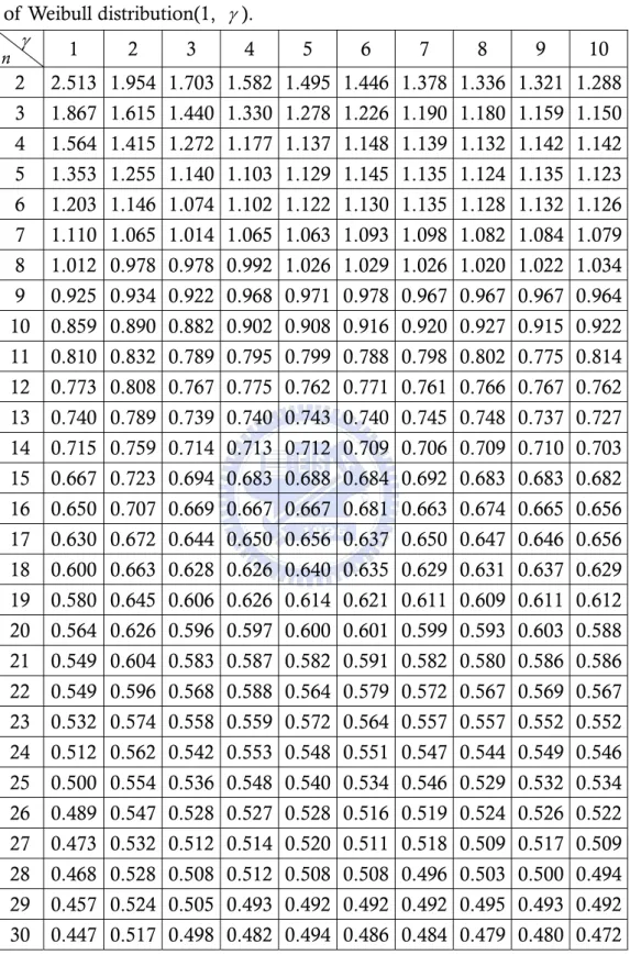
(7) List of Tables Table 1. Probabilities of detection changes in μ versus subgroup size. ................ 4 Table 2. Adjustment values for normal distribution with several subgroup size. ... 5 Table 3. AS 50 values for several subgroup sizes n and various of Gamma (N, 1)... 6 Table 4. AS 50 values for several n and various γ values when k > 0 . .................... 7 Table 5. AS 50 values for several n and various γ values when k < 0 . .................... 7 Table 6. Values of skewness and kurtosis of various Weibull distributions. ........ 10 Table 7. Detection power of the percentile Weibull control chart for k > 0 under various Weibull distributions. ............................................................. 14 Table 8. Detection power of the percentile Weibull control chart for k < 0 under various Weibull distributions. ............................................................. 14 Table 9. Detection power of the bootstrap Weibull control chart for k > 0 under various Weibull distributions. ................................................... 16 Table 10. Detection power of the bootstrap Weibull control chart for k < 0 under various Weibull distributions................................................... 16 Table 11. Detection power of the Erto’s Weibull control chart for k > 0 under various Weibull distributions. ........................................................... 20 Table 12. Detection power of the Erto’s Weibull control chart for k < 0 under various Weibull distributions. ........................................................... 20 Table 13. AS50 values for several subgroup sizes n and various γ values of Weibull distribution(1, γ ) for right shifts. ........................................ 24 Table 14. AS50 values for several subgroup sizes n and various γ values of Weibull distribution(1, γ ) for left shifts. .......................................... 25 Table 15. AS50 values for several subgroup sizes n and various γ values of Weibull distribution(1, γ ). .............................................................. 28 Table 16. The 100 observations are collected from the historical data................ 31 Table 17. goodness-of-test of wire insulation assuming normality ..................... 40 Table 18. goodness-of-test of wire insulation assuming Weibull ........................ 41. III.

(8) List of Figures Figure 1. Weibull distribution with various α .................................................. 11 Figure 2. Weibull distribution with various γ ................................................... 11 Figure 3(a)-3(j). Propability density functions for Weibull distributions along with a normal distribution for the same mean and variance..... 12 Figure 4(a)-4(j). Power curve for subgroup size 2 when α=1, γ=1(1)10, k > 0 22 Figure 5(a)-5(j). Power curve for subgroup size 2 when α=1, γ=1(1)10, k < 0 23 Figure 6. Coating layers of magnet wire insulation........................................... 29 Figure 7. Pulse voltage test. ............................................................................. 29 Figure 8. Histogram plot of the historical data. ................................................ 30 Figure 9. Normal probability plot of the historical data. ................................... 30 Figure 10(a)-10(j). Power curve for subgroup size 4 when α=1, γ=1(1)10,. k > 0 . ................................................................................. 36 Figure 11(a)-11(j). Power curve for subgroup size 6 when α=1, γ=1(1)10, k > 0 . ................................................................................. 37 Figure 12(a)-12(j). Power curve for subgroup size 4 whenα=1, γ=1(1)10, k < 0 . ................................................................................. 38 Figure 13(a)-13(j). Power curve for subgroup size 6 whenα=1, γ=1(1)10, k < 0 . ................................................................................. 39. IV.

(9) 1. Introduction 1.1. Research Background and Motivation Process capability indices (PCIs) which provide numerical measure of production characteristic to reflect the quality of product have been used in the manufacturing industry. Those indices have become popular as unit-less measures on process potential and performance. The most commonly used ones, C p and C pk discussed in Kane (1986), and more-advanced indices C pm and C pmk developed by Chan et al. (1988) and Pearn et al. (1992). Based on analyzing the PCIs, a production department can trace and improve a poor process so that the quality level can be enhanced and the requirements of the customers can be satisfied. These PCIs have been defined explicitly as:. Cp =. USL − LSL USL − LSL ⎧USL − μ μ − LSL ⎫ , C pk = min ⎨ , ⎬ , C pm = 6σ 3σ ⎭ ⎩ 3σ 6 σ 2 + ( μ −T )2 ⎧⎪ USL − μ μ − LSL C pmk = min ⎨ , 2 2 2 2 ⎩⎪ 3 σ + ( μ − T ) 3 σ + ( μ − T ). ⎫⎪ ⎬, ⎭⎪. where USL is the upper specification limit, LSL is the lower specification limit, μ is the process mean, σ is the process standard deviation, and T is the target value. The index C p considers the overall process variability relative to the manufacturing tolerance, reflecting product quality consistency. The index C pk takes the magnitude of process variance as well as process departure from target value, and has been regarded as a yield-based index since it providing lower bounds on process yield, and is always used to measure the quality of the process. When data come from normal distribution, for a C pk level of 1, statistically one would expect that the product’s fractions of defectives, is no more than 2700 parts per million (ppm) fall outside the specification limits. At C pk =1.33, the defect rate drops to 66 ppm. To attain less than 0.544 ppm defect rate, a C pk level of 1.67 is required. At a C pk level of 2.0, the defective rate reduced to 0.002 ppm. The exact number of nonconformities with fixed C pk is very depending upon the location of the process mean and the magnitude of the process variation. C pk is calculated under assumptions that the process is stable (the process mean and variation are not change), but in practice, the process is dynamic and the mean and variation always change with small movement for momentary, and the some control charts can’t detect obviously so that the C pk will underestimated the true number of nonconformities. The changes of various magnitudes not only happen on normal distribution, but also on non-normal distribution. Pyzdek (1995) has mentioned the distributions of certain chemical processes such as zinc plating thickness of a hot-dip galvanizing process are very quite often skewed. Choi (1996) presents an example of a skewed distribution in the ‘active area’ shaping stage of the wafer’s production process. Cygan et al. (1989) have mentioned that the lifetimes of 1.

(10) polypropylene films under high ac and dc field stresses be shown as a two-parameter Weibull distribution. The Weibull distribution, denoted as Weibull ( α , γ ), with various values of scale parameter α and shape parameter γ , covers a wide class of non-normal applications, including product life, product reliability and tensile strength of brittle materials, such as carbon and boron. The abundance of outputs from skewed distribution, the censoring, etc, makes the normality assumption often being illegitimate. Specifically, we assure the product lifetime which be from skewed distribution by statistic test and historical data. It will lead to underrate the probability of nonconformance that using the adjustment for normal case to adjust the non-normal cases. 1.2. Research Purpose and Objectives Ever since Motorola, Inc. introduced its Six Sigma quality initiative, followers of this philosophy notion should add 1.5 σ when estimating process capability. By this idea we will find that 6-sigma actually translates to about 2 defects per billion opportunities, and 3.4 defects per million opportunities, which we normally define as Six Sigma, really corresponds to a sigma value of 4.5. When asked the reason for such an adjustment, six-sigma user claim it is necessary, but offer only personal experiences and three dated empirical literature. Bothe (2002) provided a statistical reason to adjust the overestimated C pk . Bothe set the adjustment of shift in average that was dependent on the same detection power of the control chart, and the data of Bothe’s study was assumed to be approximately normality distribution. However effectively non-normal process occurs frequently in practice. If the process capability indices based on the normal assumption concerning the data are used with non-normal observations, the value of the process capability indices may, in a majority of situation, be incorrect and quite likely misrepresent the actual product quality. The control charts are commonly used in many industries for providing early warning for the shift in process mean. If the control chart detects a process mean shift, then the process is not under control. The well-known and usual Shewhart X control charts assume that the observed process data come from a near-normal distribution. However, when the process distribution is unknown or non-normal, the parameter estimators of sampling distribution may not be available theoretically. We can use approximation or simulation to estimate the parameters, such as percentile Weibull control chart which uses simulation to get the UCL (upper control limits) and LCL (lower control limits). But for Weibull processes, Erto (2007) used Bayes theorem to provide a Weibull control chart. If data come from Weibull distribution, we can control the process more exactly than non-normal control chart. In this research, we show that the detection power performance of three Weibull control charts under the same mean shift adjustment which Bothe provided when the processes in control is very sensitive to the assumption of normality. Then, we compare with the detection power performances of the three control charts. Using the most powerful control chart to provide the statistical derived mean shift adjustment based on the chart subgroup size and distribution 2.

(11) parameter to calculate the estimator of C pk when the data is non-normal distribution for Weibull distribution. 1.3. Thesis Organization First, we introduce the research motivation and purpose in Chapter 1. Secondly, a brief introduction of Bothe’s study and adjustment reason are included and adjustment for Gamma processes and Weibull processes in Chapter 2. In Chapter 3, we introduce the characteristic of Weibull distribution, and introduce some Weibull control charts for Weibull processes, and calculate the detection powers of control charts under the same shift for Weibull processes. We compare the detection powers to choose the best one. After that we calculate the adjustment for Weibull processes by using the best powerful Weibull control chart. In Chapter 4, we introduce the calculation of dynamic non-normal index C pk , and show the dynamic C pk for Weibull processes. For illustrative purpose, an application is presented in Chapter 5. Finally, we give some conclusions in Chapter 6.. 3.

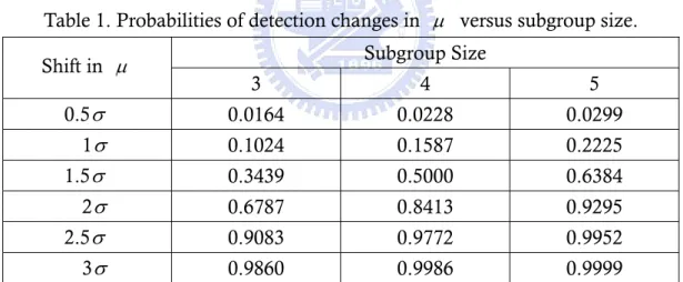
(12) 2. Literature Review The processes capability adjustment for normal and non-normal distributions had been researched. In this section, we will review these papers about adjustments for normal processes, Gamma processes and Weibull processes. 2.1. Process Capability Adjustment for Normal Processes Bothe (2002) provided a statistical reason why to add a 1.5 σ shift to the average. Assuming the processes approximately normal distribution, control charts can’t reliably detect small movement in average. Table 1 displays the probabilities of detecting changes in μ versus subgroup size for shift=0.5(0.5)3 σ with n=3, 4 and 5. When μ had a small movement (ex: 0.5 σ , 1 σ ) and the detection power of Shewhart X control chart is too small to discover. Then, small mean movement affects the PCIs accuracy. However, the probability of nonconformance will increase obviously. For example, when C pk is 1.33, the probability of nonconformance is 64 ppm. If average occur 1 σ shift that be difficultly detected by control chart, the probability of nonconformance becomes 1350 ppm. The probability of nonconformance will increase twenty-fold. Bothe considered that adjustments should accord with the same detection standard. Table 1. Probabilities of detection changes in μ versus subgroup size. Shift in μ. Subgroup Size 3. 4. 5. 0.5 σ. 0.0164. 0.0228. 0.0299. 1σ. 0.1024. 0.1587. 0.2225. 1.5 σ. 0.3439. 0.5000. 0.6384. 2σ. 0.6787. 0.8413. 0.9295. 2.5 σ. 0.9083. 0.9772. 0.9952. 3σ. 0.9860. 0.9986. 0.9999. When subgroup size is 4 and mean shift is 1.5 σ , the detecting power will be 0.5. Bothe (2002) considered providing the same detecting power in order to define the several adjustments with different subgroup size and called the adjustments S 50 . By this idea, he set the detecting power to 50 percent and computed the several adjustments for different subgroup size. The reason which Bothe set the power to 50 percent was we want detect the processes out of control immediately if the process mean shifts and the ARL1 (average run length)=1 is the perfect condition. But in fact, the ARL1 = 1 is impossible. For this reason we can just only set the ARL1 = 2 , and the detection power is 1 ARL1 , so we can know if ARL1 = 2 the detecting power is 0.5. The results showed in Table 2. 4.

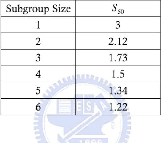
(13) Table 2 displays shift sizes that have 50 percent chance of remaining undetected for subgroup sizes 1 through 6. Because shifts ranging in size from 0 up to S 50σ are the ones likely to remain undetected, a conservative approach is to assume that every missed shift is as large as S 50σ . And Bothe invented dynamic C pk be defined as ⎡USL − ( μ + S50σ ) ( μ − S50σ ) − LSL ⎤ dynamic C pk = min ⎢ , ⎥. 3σ 3σ ⎣ ⎦. The dynamic C pk could be corrected by subgroup size really not fixed 1.5σ adjustment.. Table 2. Adjustment values for normal distribution with several subgroup size. Subgroup Size. S 50. 1. 3. 2. 2.12. 3. 1.73. 4. 1.5. 5. 1.34. 6. 1.22. 2.2. Process Capability Adjustment for Gamma Processes When using the index C pk , one of the most essential is that the process monitored is supposed to be stable and the output is approximately normally distributed. When the distribution of a process characteristic is non-normal, PCIs calculated using conventional methods could often lead to erroneous and misleading interpretation of the process’s capability. In the recent years, several approaches to the problems of PCIs for the non-normal populations have been suggested (see e.g. Pal (2005), Ding (2004), Pearn and Chen (1997), Kotz and Lovelace (1998), Somerville and Montgomery (1996), Kocherlakota and Kirmani (1992)). Several authors used data transformation techniques such as the Box-Cox power transformation, Johnson’s transformations and quantile transform techniques to solve this problem. And some authors replaced the unknown distribution by a known three or four-parameter distribution. Examples include Clments (1989), Franklin and Wasserman (1992), Shore (1998) and Polansky (1998). Hsu et al. (2007) provided the process capability adjustment for gamma process. For small process mean shifts, it is beyond the control chart detection power when process assumed gamma distribution and the process capability will be overestimated. They examine Bothe’s approach and find the detection power was less than 0.5 when data came from gamma distribution, showing that Bothe’s 5.

(14) adjustments are inadequate when we had gamma processes. Then, they calculate adjustments which called AS50 under various sample sizes n and gamma parameter N , with power fixed to 0.5. Table 3 displays the magnitude of adjustments AS50 which they provided and data comes from Gamma ( N , 1 ) with various values of N = 1(1)10 and n = 2(1)10 . Table 3. AS50 values for several subgroup sizes n and various of Gamma(N, 1). 1. 2. 3. 4. 5. 6. 7. 8. 9. 10 N(0,1). 2. 3.611 3.185 2.992 2.876 2.797 2.738 2.692 2.655 2.625 2.599 2.12. 3. 2.732 2.443 2.313 2.236 2.182 2.143 2.113 2.088 2.067 2.050 1.73. 4. 2.252 2.034 1.936 1.878 1.838 1.808 1.785 1.767 1.752 1.738. 5. 1.944 1.769 1.690 1.644 1.612 1.588 1.570 1.555 1.543 1.532 1.34. 6. 1.727 1.581 1.515 1.476 1.450 1.430 1.415 1.403 1.392 1.384 1.22. 7. 1.565 1.439 1.383 1.350 1.327 1.310 1.297 1.286 1.278 1.270 1.13. 8. 1.438 1.328 1.279 1.249 1.229 1.215 1.203 1.194 1.186 1.180 1.06. 9. 1.336 1.237 1.194 1.168 1.150 1.137 1.127 1.118 1.112 1.106 1.00. 10. 1.251 1.162 1.123 1.100 1.084 1.072 1.063 1.055 1.049 1.044 0.95. 1.5. Hsu et al. (2007) used the most common method for modifying PCIs in the non-normal case is the technique of quantile estimation. Analogous to the normal case, where the “natural” process width is between the 0.135th percentile and the 99.865th percentile, PCIs can be redefined in terms of their quantiles for possible modification in the non-normal case. The quantile definition for C pk are defined as: C pk = min {C pu , C pl }. ⎧ USL − F0.5 F − LSL ⎫ =min ⎨ , 0.5 ⎬, ⎩ F0.99865 − F0.5 F0.5 − F0.00135 ⎭ so that the normality assumption can be verified simultaneously. To consider the undetected process mean shift, they obtained Dynamic C pk index for non-normal process by modifying Bothe’s Dynamic C pk :. ⎧USL − ( F0.5 + AS50σ ) ( F0.5 − AS50σ ) − LSL ⎫ , dynamic C pk =min ⎨ ⎬. F0.99865 − F0.5 F0.5 − F0.00135 ⎩ ⎭ By considering an adjustment AS50σ in this assessment for undetected shifts in process median, the estimate of dynamic index C pk will decrease and the expected total number of nonconforming parts will increase. This nonconforming level assumes that undetected shifts are happening almost constantly and that every one is equal to AS50σ . 6.

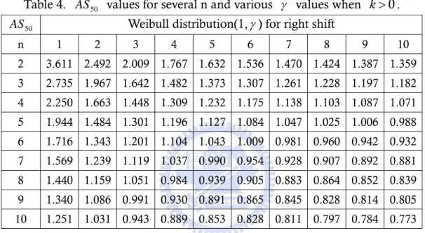
(15) 2.3. Process Capability Adjustment for Weibull Processes Li (2007) provided the process capability adjustment for Weibull process. Weibull distribution doesn’t have reproductive, and the parameter of the X distribution can’t be found easily. They used a reference which Lu (2003) provided to approximate the cumulative density function of X n of Weibull processes. The UCL and LCL was 99.865th and 0.135th percentile of X n distribution. We call the control chart they used is percentile Weibull control chart. Then they used the control limits to calculate the detection power for Weibull processes under the subgroup size n and shape parameter γ . Table 4. AS 50 values for several n and various γ values when k > 0 . Weibull distribution(1, γ ) for right shift. AS 50 n. 1. 2. 3. 4. 5. 6. 7. 8. 9. 10. 2. 3.611 2.492 2.009 1.767 1.632 1.536 1.470 1.424 1.387 1.359. 3. 2.735 1.967 1.642 1.482 1.373 1.307 1.261 1.228 1.197 1.182. 4. 2.250 1.663 1.448 1.309 1.232 1.175 1.138 1.103 1.087 1.071. 5. 1.944 1.484 1.301 1.196 1.127 1.084 1.047 1.025 1.006 0.988. 6. 1.716 1.343 1.201 1.104 1.043 1.009 0.981 0.960 0.942 0.932. 7. 1.569 1.239 1.119 1.037 0.990 0.954 0.928 0.907 0.892 0.881. 8. 1.440 1.159 1.051 0.984 0.939 0.905 0.883 0.864 0.852 0.839. 9. 1.340 1.086 0.991 0.930 0.891 0.865 0.845 0.828 0.814 0.805. 10. 1.251 1.031 0.943 0.889 0.853 0.828 0.811 0.797 0.784 0.773. Table 5. AS 50 values for several n and various γ values when k < 0 . Weibull distribution(1, γ ) for left shift. AS 50 n. 1. 2. 3. 4. 5. 6. 7. 8. 9. 10. 2. 0.820 1.532 1.888 2.098 2.236 2.333 2.405 2.461 2.504 2.540. 3. 0.813 1.356 1.591 1.723 1.808 1.866 1.909 1.941 1.967 1.987. 4. 0.802 1.225 1.399 1.494 1.554 1.596 1.626 1.649 1.667 1.681. 5. 0.776 1.125 1.263 1.337 1.384 1.416 1.439 1.456 1.470 1.481. 6. 0.749 1.047 1.160 1.221 1.259 1.285 1.304 1.318 1.329 1.338. 7. 0.724 0.983 1.079 1.131 1.163 1.185 1.201 1.213 1.222 1.230. 8. 0.700 0.929 1.013 1.058 1.086 1.105 1.118 1.129 1.137 1.144. 9. 0.678 0.884 0.958 0.998 1.022 1.039 1.051 1.060 1.067 1.073. 10. 0.658 0.844 0.911 0.947 0.969 0.984 0.994 1.003 1.009 1.014. Since the shape of the Weibull distribution changing from positive skewness to negative skewness with increasing the shape parameter, they discussed two different cases. Process mean had right and left shifts. They used this cumulative 7.

(16) density function to compute the relationship between the mean shift and Type Ⅱ error and calculate the mean shift adjustment AS50 which means that the processes mean shift AS50 sigma when the detection power of control chart is 0.5. Table 4 and Table 5 display the magnitude of mean shift adjustments AS 50 based on the detection power is 0.5 and data from Weibull ( 1, γ ) distribution for various value of γ = 1(1)10 and n=2(1)10 with right shift ( k > 0 ) and left shift ( k < 0 ). They also used the most common method for modifying PCIs in the non-normal case is the technique of quantile estimation, and the dynamic C pk was as the same as gamma processes which Hsu et al. (2007) provided. The adjustments of Weibull processes are related that which control chart you choose to control the process. The Shwehart X control chart assumed that the process data come from a normal or near-normal distribution. When the data come from Weibull distribution, we should choose control charts for non-normal processes or for Weibull processes to control production process. Padgett and Supurrier (1990) use Monte Carlo simulation to construct Shewhart-type control charts for percentiles of strength distributions. Chan and Cui (2003) provided a skewness correction X and R charts for skewed distribution. This control chart proposed a skewness correction method for constructing the X and R control charts for skewed process distributions. Their asymmetric control limits are based on the degree of skewness estimated from the subgroups. Nichols and Padgett (2006) provided a bootstrap Weibull control chart. This control chart is use bootstrap method to simulate the UCL and LCL for monitoring Weibull percentiles. Erto (2006) provided a Weibull control chart which was used Bayes theorem to calculate the sampling distribution of Weibull percentile.. 8.

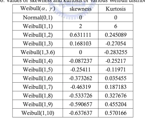
(17) 3. Control Chart Power Analysis for Weibull Processes In this section, we introduce the Weibull distribution, and use three control charts for Weibull processes to calculate the detection powers. Then, we analysis the detection powers and compare them to find the best powerful control chart to calculate the adjustments for Weibull processes. 3.1. The Weibull Processes The Weibull distribution has been often used in the field of life data analysis due to its flexibility. It can mimic the behavior of other statistical distributions such as the normal and the exponential. The Weibull distributions are also used to model the time until a given technical device fails. If the failurerate of the device decreases over time, one chooses γ < 1 ( γ is the shape parameter). If the failure rate of the device is constant over time, one choose γ = 1 , again resulting in a decreasing function f. If the failure rate of the device increases over time, one chooses γ > 1 and obtains a density f which increases towards a maximum and then decreases forever. The Weibull distribution is non-negative distribution. It can be denoted as Weibull ( α , γ ) with scale parameter α and shape parameter γ . The cumulative density function function is defined as γ. F ( X ) = 1-e− ( x / a ) , x > 0, α > 0, γ > 0,. (1). and the probability density is. f ( x ) = γα −γ x γ −1e. x − ( )γ. α. , x > 0, α > 0, γ > 0,. (2). The mean and variance are given, respective, by. μ = α [Γ(1 + γ -1 )],. (3). σ 2 = α 2 [Γ(1 + 2γ -1 ) - Γ 2 (1 + γ -1 )].. (4). and. Denoting the Weibull distribution is skewed. To know how this distribution are different from the normal distribution in term of the coefficient of skewness and the coefficient of kurtosis of the Weibull distribution under study are presented in Table 3. The coefficient of skewness Weibull distribution is given by:. γ1 =. 2Γ3 (1 + γ −1 ) − 3Γ(1 + γ −1 )Γ(1 + 2γ −1 ) + Γ(1 + 3γ −1 ) , [Γ(1 + 2γ −1 ) − Γ 2 (1 + γ −1 )]3/2. (5). The kurtosis coefficient of Weibull distribution is given by:. γ2 =. f (γ ) , [Γ(1 + 2γ ) - Γ 2 (1 + γ -1 )]2 -1. 9. (6).

(18) where Γ (x ) is the gamma function and. f (γ ) ≡ −6Γ 4 (1 + γ −1 ) + 12Γ 2 (1 + γ −1 )Γ(1 + 2γ −1 ) −. 3Γ 2 (1 + 2γ −1 ) − 4Γ(1 + γ −1 )Γ(1 + 3γ −1 ) + Γ(1 + 4γ −1 ).. (7). The Equations (5) and (6) show that skewness coefficient and the kurtosis coefficient are calculated only by using the shape parameter γ . This means that the scale parameter α can not affect the values of skewness and kurtosis of Weibull distributions. Therefore, we fix α = 1 in this study for the Weibull distributions. To see how this distribution are different from the standard normal distribution in terms of skewness and kurtosis, Table 6 shows the values of skewness and kurtosis (which are defined as the third and fourth moments of the standardized distribution, respectively) of the Weibull distributions under study. It can be found in Table 6 that when the value of γ increases from 1 to 3.6, the corresponding values of skewness will become smaller and close to 0. Especially, when value of γ is 3.6, the skewness coefficient of the Weibull distribution is 0. This means the Weibull (1, 3.6) distribution is symmetric about median and appears more nearly normal distribution. When the value of γ increases form 3.6 to 10, the corresponding values of skewness will become negative and far from to 0. From the results through these distributions, we can get some insights of the effects of non-normality in terms of skewness and kurtosis.. Table 6. Values of skewness and kurtosis of various Weibull distributions. Weibull( α , γ ) skewness Kurtosis Normal(0,1). 0. 0. Weibull(1,1). 2. 6. Weibull(1,2). 0.631111. 0.245089. Weibull(1,3). 0.168103. -0.27054. Weibull(1,3.6). 0. -0.283255. Weibull(1,4). -0.087237. -0.25217. Weibull(1,5). -0.25411. -0.11971. Weibull(1,6). -0.373262. 0.035455. Weibull(1,7). -0.46319. 0.187183. Weibull(1,8). -0.533726. 0.327676. Weibull(1,9). -0.590657. 0.455204. Weibull(1,10). -0.637637. 0.570166. The formula of these modulus let us know that α is scale parameter and γ is shape parameter. To make short of the matter, scale parameter can modulate the fold of the mean and the variance. Figure 1 displays Weibull distribution with 10.

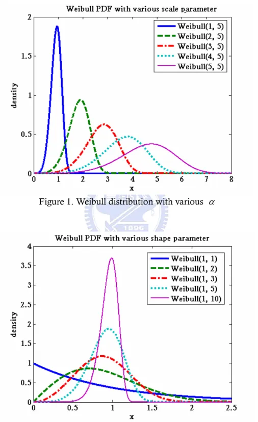
(19) various values of α and Figure 2 displays Weibull distribution with various of γ . We can find the scale parameter only control the mean and the variance to adjust the distribution size.. Figure 1. Weibull distribution with various α. Figure 2. Weibull distribution with various γ. 11.

(20) Figure 3(a)-3(j). Propability density functions for Weibull distributions along with a normal distribution for the same mean and variance. 12.

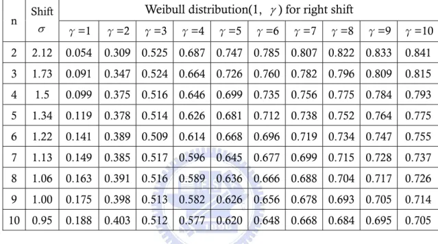
(21) Figure 3 shows several Weibull distributions along with a normal distribution for the same mean and variance. In this study, we let γ = 1(1)10, while (without loss of generality) fixing α = 1 . In Figure 3(a)-3(j) with the increasing value of γ , the Weibull (1,3) and Weibull (1,4) distributions appear more nearly normal distribution. In fact, we demonstrate this convergence property in Table 6 by calculating the skewness and kurtosis. It can be seen that as the value of γ in the region of [3, 4], the skewness and kurtosis of Weibull distribution will be getting much closer to those of normal distribution. This fact could be also found according to Equation (10). When the value of γ in the region of of [3, 4], the form of Weibull distribution becomes centralizing. Through these distributions, we wish to get some insights of the effects of non-normality on the detection power in terms of skewness and kurtosis in Section 3. 3.2. The Detection Power of the Percentile Weibull Control Chart In this section we use percentile Weibull control chart to calculate the detection power. Let X 1 , X 2 ,K, X n be a sequence observations of independent and identically distributed in Weibull ( α , γ ). The detection power was defined the probability of outline control chart under the mean being shifted. Its mean 1-type Ⅱ error β . The detection power is:. Detection power = 1-P ( LCL ≤ X n ≤ UCL μ1 = μ0 + kσ x ) = 1-P ( FX (0.00135) ≤ X n ≤ FX (0.99865) μ1 = μ0 + kσ x ),. (8). where μ1 is the mean after process shift ( μ 0 is the mean of the original process). The control limits LCL and UCL are calculated as FX n (0.00135) and FX n (0.99865) respectively, where FX n (0.00135) and FX n (0.99865) are 0.135th percentile and 99.865th of X of sampling distribution. We can obtain the approximate c.d.f. of X n distribution by a reference which Li (2007) provided. Since the X n distribution is not symmetric, we discussed μ occurred right movement and left movement. When k > 0 , it is mean μ occurred right movement; and k < 0 means μ occurred left movement. Table 7 and Table 8 display the detection power with right process mean shift ( k > 0 ) and left process mean shift ( k < 0 ) when X 1 , X 2 ,K, X n come from Weibull ( α , γ ) with α = 1 and γ = 1 (1) 10 , and the number of subgroup is 100000. The magnitude of shift in the second column on the left is Bothe’s capability adjustments determined when data comes from normal distribution and the detection power is 0.5. We can find that the detection power is less than 0.5 when γ = 1 and 2 in Table 7, and γ ≥ 5 in Table 8 under Bothe’s capability adjustments. The results show that the Bothe’s adjustments are inadequate when we have Weibull processes. This is due to Bothe’s approach is based on the normality assumption of the data and the detection power is 0.5. The detection power is more than 0.5 when γ = 3 and 4 in Tables 7 and 8. This means that Weibull distribution is close to normal distribution when γ = 3 and 4. This fact could be also found from Table 6 and Figures 3(c)-3(d). As the value of γ in the region of of [3, 4], the form of Weibull distribution becomes centralizing. 13.

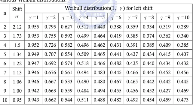
(22) However, the detection power is poorer and far less than 0.5 when data come from more skewed Weibull distribution. For example, when γ = 1 and the subgroup size n = 2 , the detection power is 0.054. It implies Bothe’s adjustments are inadequate when we have skewed processes. Consequently, in our study, we determined the capability adjustment when process data comes from Weibull distribution. Table 7. Detection power of the percentile Weibull control chart for k > 0 under various Weibull distributions. Weibull distribution(1, γ ) for right shift. n. Shift σ. γ=1. γ=2. γ=9. γ=10. 2. 2.12. 0.054. 0.309 0.525 0.687 0.747 0.785 0.807 0.822 0.833. 0.841. 3. 1.73. 0.091. 0.347 0.524 0.664 0.726 0.760 0.782 0.796 0.809. 0.815. 4. 1.5. 0.099. 0.375 0.516 0.646 0.699 0.735 0.756 0.775 0.784. 0.793. 5. 1.34. 0.119. 0.378 0.514 0.626 0.681 0.712 0.738 0.752 0.764. 0.775. 6. 1.22. 0.141. 0.389 0.509 0.614 0.668 0.696 0.719 0.734 0.747. 0.755. 7. 1.13. 0.149. 0.385 0.517 0.596 0.645 0.677 0.699 0.715 0.728. 0.737. 8. 1.06. 0.163. 0.391 0.516 0.589 0.636 0.666 0.688 0.704 0.717. 0.726. 9. 1.00. 0.175. 0.398 0.513 0.582 0.626 0.656 0.678 0.693 0.705. 0.714. 10. 0.95. 0.188. 0.403 0.512 0.577 0.620 0.648 0.668 0.684 0.695. 0.705. γ=3. γ=4. γ=5. γ=6. γ=7. γ=8. Table 8. Detection power of the percentile Weibull control chart for k < 0 under various Weibull distributions. Weibull distribution(1, γ ) for left shift Shift n. σ. γ=1. γ=2. γ=3. γ=4. γ=5. γ=6. γ=7. γ=8. γ=9. γ=10. 2. 2.12. 0.928 0.782 0.550 0.513 0.439 0.387 0.350 0.323 0.304 0.288. 3. 1.73. 0.906 0.733 0.537 0.506 0.449 0.411 0.384 0.364 0.348 0.337. 4. 1.5. 0.886 0.702 0.532 0.505 0.458 0.426 0.404 0.385 0.375 0.365. 5. 1.34. 0.868 0.680 0.527 0.504 0.464 0.436 0.416 0.401 0.390 0.381. 6. 1.22. 0.852 0.664 0.525 0.504 0.467 0.441 0.424 0.411 0.401 0.393. 7. 1.13. 0.836 0.649 0.553 0.499 0.466 0.443 0.427 0.416 0.406 0.399. 8. 1.06. 0.825 0.642 0.552 0.502 0.471 0.450 0.436 0.424 0.416 0.409. 9. 1.00. 0.814 0.634 0.549 0.503 0.474 0.454 0.440 0.430 0.422 0.415. 10. 0.95. 0.805 0.629 0.548 0.504 0.477 0.458 0.445 0.435 0.427 0.421. 14.

(23) 3.3. The Detection Power of the Bootstrap Weibull control chart The usual Shewhart control charts assume that the observed process data come from a near-normal distribution. However, when the distribution of the process under observation is unknown or non-normal such as Gamma or Weibull, the sampling distribution of a parameter estimator may not be available theoretically. One of the ways to estimate parameter is simulation. Nichols and Padgett (2006) provided a bootstrap Weibull control chart for Weibull percentiles. This control chart is use bootstrap method to construct control chart limits for monitoring a specified percentile of the process distribution. The percentile of the Weibull distribution is 1. W p = α [ − ln(1 − p )]γ , 0 < p <1, where W p is the 100 p. th. percentile.. The following steps are used to construct the bootstrap Weibull control chart. 1.. From an in-control, stable process, observe n × m observations taken from Weibull distribution with unknown scale and shape parameters, α and γ , respectively. The observations are denoted by x ij , i = 1,K, n, and j = 1,K, m, and are assumed to come from m independent subgroups of size n .. 2.. Using the maximum likelihood method to find αˆ and γˆ . The equations are ⎡ ∑ m ∑ n x ijγ ln x i ∑ m ∑ n x ijγ ln x i ⎤ ⎥ γ = ⎢ j =1 m i =1 n γ − j =1 i =1 nm ⎢ ∑ ∑ x ij ⎥ j =1 i =1 ⎣ ⎦. −1. ⎡ ∑ m ∑ n x ijγ and α = ⎢ j =1 i =1 nm ⎢ ⎣. 1. ⎤γ ⎥ . ⎥ ⎦. 3.. Generate a bootstrap subgroup of size n, x1* , x 2* ,K x n* , from the Weibull distribution using maximum likelihood estimators, αˆ and γˆ , as the estimated parameters.. 4.. Find the parameter MLEs from the bootstrap subgroup and denote these as αˆ * and γˆ * .. 5.. For the bootstrap subgroup, find W p = αˆ * [ − ln(1 − p )] γˆ , 0 < p <1, the bootstrap estimate of the 100 p th percentile, W p .. 6.. Repeat steps 3-5 a large number of times, B , obtaining B bootstrap estimates of W p , denoted by W p*1, W p*2 , K, W p*B .. 7.. Order the B bootstrap estimates W pi* , from smallest to largest. The LCL is the ( 0.00135 × B ) value of the ordered W pi* , and the UCL is the ( 0.99865 × B ) value of the ordered W pi* .. 1. 15. *.

(24) Table 9. Detection power of the bootstrap Weibull control chart for k > 0 under various Weibull distributions. Weibull distribution(1, γ ) for right shift. n. Shift σ. γ=1. γ=2. γ=9. γ=10. 2. 2.12. 0.066. 0.283 0.489 0.572 0.642 0.679 0.717 0.733 0.755. 0.758. 3. 1.73. 0.118. 0.306 0.456 0.574 0.644 0.669 0.702 0.710 0.721. 0.743. 4. 1.5. 0.180. 0.329 0.476 0.574 0.617 0.646 0.666 0.698 0.716. 0.727. 5. 1.34. 0.169. 0.355 0.461 0.543 0.603 0.638 0.669 0.673 0.688. 0.722. 6. 1.22. 0.256. 0.344 0.488 0.541 0.581 0.626 0.661 0.674 0.697. 0.704. 7. 1.13. 0.289. 0.363 0.488 0.538 0.581 0.618 0.652 0.676 0.678. 0.705. 8. 1.06. 0.305. 0.381 0.470 0.538 0.592 0.616 0.656 0.659 0.682. 0.691. 9. 1.00. 0.343. 0.384 0.480 0.547 0.581 0.612 0.643 0.656 0.676. 0.688. 10. 0.95. 0.361. 0.395 0.491 0.552 0.580 0.634 0.640 0.658 0.682. 0.683. γ=3. γ=4. γ=5. γ=6. γ=7. γ=8. Table 10. Detection power of the bootstrap Weibull control chart for k < 0 under various Weibull distributions. Weibull distribution(1, γ ) for left shift. n. Shift σ. γ=1. γ=2. γ=9. γ=10. 2. 2.12. 0.955. 0.795 0.627 0.512 0.440 0.388 0.359 0.334 0.319. 0.289. 3. 1.73. 0.953. 0.755 0.592 0.499 0.464 0.419 0.385 0.374 0.362. 0.340. 4. 1.5. 0.952. 0.726 0.582 0.496 0.462 0.431 0.391 0.385 0.409. 0.385. 5. 1.34. 0.949. 0.707 0.554 0.509 0.465 0.441 0.437 0.434 0.415. 0.407. 6. 1.22. 0.947. 0.692 0.574 0.518 0.466 0.482 0.435 0.440 0.434. 0.432. 7. 1.13. 0.946. 0.676 0.561 0.494 0.483 0.445 0.466 0.446 0.452. 0.456. 8. 1.06. 0.946. 0.667 0.533 0.490 0.480 0.467 0.465 0.442 0.442. 0.445. 9. 1.00. 0.942. 0.663 0.559 0.484 0.494 0.455 0.456 0.452 0.427. 0.469. 10. 0.95. 0.943. 0.662 0.544 0.511 0.488 0.482 0.492 0.454 0.459. 0.473. γ=3. γ=4. γ=5. γ=6. γ=7. γ=8. In order to compare with the detection power of the percentile Weibull control chart, we set the percentile p to be 0.5 to similar the sampling distribution of X n and the repeated time B is 100000. Table 9 and Table 10 display the detection power of the 50th percentile of the distribution with shift kσ x when data come from Weibull distribution with the scale parameter α = 1 and the shape parameter γ = 1 (1) 10 . The shift distance in the second column is 16.

(25) Bothe’s adjustment as the same as Table7 and Table 8. We can find that the detection power is less than 0.5 when γ ≤ 3 in Table 9, and γ ≥ 5 in Table 10. This results show that the Bothe’s adjustments are inadequate too as the same as the results in Section 3.2, and when data come from more skewed Weibull distribution, we have also the same results in Section 3.2 that the detection power is poorer and far less than 0.5. 3.4. Erto’s Weibull Control Chart for Weibull Processes In past section we talk about the Shewhart X control chart assumed that data should come from normal distribution. If data come from non-normal distribution (such as Gamma or Weibull distribution), we just only use simulation or approximate to get an inexact results. In order to get an exact result, using a Weibull control chart which Erto (2006) provided is a better choice. Erto provided a new Shewhart-type control chart of Weibull percentile. This chart uses Practical Bayes Estimators (PBE) of the Bayes theorem to integrate both technological and statistical information analytically. The PBE were developed from engineers’ point of view. The Weibull survival function is: Sf { x ; α , γ } = exp ⎡⎣ −( x α )γ ⎤⎦ ;. α , γ > 0,. x ≥ 0;. (9). where α , γ are scale and shape parameters of the Weibull distribution. We can be immediately reparameterized in terms of the percentile x R and shape parameter β , in which the Engineers’ knowledge can be more easily converted: Sf { x ; x R , γ } = exp ⎡⎣ − K ( x x R )γ ⎤⎦ , x ≥ 0, x R , γ > 0, K = ln(1 R ),. (10). where x R and γ both being unknown. x R is equivalent to the 1 − R percentile of the Weibull distribution, for example: if R = 0.90 and x R = 1,000 hours, then 90% of the items have lives greater than 1,000 hours. The uniform prior probability density function in the interval ( γ 1 , γ 2 ) is assumed to fit the degree of belief in the shape parameter β of the sampling distribution:. ⎧1 ( γ 2 − γ 1 ) ; γ 2 ≥ γ ≥ γ 1 > 0; pdf{γ } = ⎨ ⎩0; elsewhere. γ 2 > γ1. ,. (11). it appears to be as non-restrictive as feasible. For the selected percentile x R (corresponding to the fixed reliability level R ) the prior probability density function is assumed to be the Inverse Weibull: pdf{x R } = a b (a x R ) − ( b +1) exp ⎡⎣ −(a x R ) − b ⎤⎦ ;. 17. x R ≥ 0;. a, b > 0,. (12).

(26) where a and b are scale and shape parameters respectively. It is assumed b = γ . When the greater γ is, the more peaked the Weibull probability density function is, the smaller the uncertainty in x R is and then greater b must be, so b = γ is the simplest choice. So the probability density function of x R is converted into the conditional prior: pdf { x R γ } = a γ (a x R ) − ( γ +1) exp ⎡⎣ − (a x R ) − γ ⎤⎦ ;. a, γ > 0.. (13). From Equation (11), the mean value E { x R } of the probability density function is: E { x R } = (1 a ) Γ(1 − 1 b ). From this function and assumed b = γ , we can know that:. a=. Γ(1 − 1 γ m ) ; E {x R }. γ m = (γ 1 + γ 2 ) 2.. (14). Usually, a sample array x of n experimental data is available. If the reliability (measured in terms of lifetime, tensile strength, breaking strength, etc.) of the items is characterized by the Equation (9), the likelihood of the sample is given by: n. ⎛ γ ⎞ n ⎛ K n L(x x R , γ ) ∝ ⎜ γ ⎟ ∏ x iγ −1 exp ⎜ − γ ∑ x iγ ⎝ x R ⎠ i =1 ⎝ x R i =1. ⎞ ⎟. ⎠. (15). And from the two priors Equation (10) and (12), the joint probability density function of x R and γ is obtained: pdf{x R , γ } = (γ 2 − γ 1 ) −1 a γ (a x R ) − (γ +1) exp ⎡⎣ −(a x R ) − γ ⎤⎦ .. (16). Combining the Equation (14) and (15) by using the Bayes theorem which substantially says: ⎛ joint posterior probability density ⎞ ⎛ their joint prior ⎞ ⎛ likelihood ⎞ ⎜ ⎟∝⎜ ⎟×⎜ ⎟ ⎝ of unknown parameters ⎠ ⎝ probability density ⎠ ⎝ function ⎠ “Prior” and “posterior” mean before and after obtaining experimental data respectively. So, in this way, the theorem fuses the technological prior knowledge, summarized into joint prior, with all the information (data and shape of the reliability model) included into likelihood. We can get the joint posterior probability density function of unknown parameters is:. pdf { x R , γ x } =. n ⎡ ⎞⎤ γ −1 −γ ⎛ −γ x exp x a K x iγ ⎟ ⎥ − + ∑ ∏ i ⎢ R ⎜ i =1 ⎝ ⎠⎦ i =1 ⎣ . (17) n − ( + 1) n n γ −1 ⎛ − γ γ ⎞ xi ⎜ a + K ∑ xi ⎟ dγ ∏ i =1 ⎝ ⎠ i =1. γ n +1 a −γ x R −γ ( n +1) −1 γ2. n ! ∫ γ n a −γ γ1. n. 18.

(27) From Equation (16), we can calculate the expectations of x R and γ is: E {x R x } =. I3 ; I1. E {γ x } =. I2 , I1. (18). where γ2. Ij =∫ γ a γ1. mj. −γ. n. ∏x i =1. γ −1 i. n ⎛ −γ γ ⎞ ⎜ a + K ∑ xi ⎟ i =1 ⎝ ⎠. − ( n +1) + k j. Γ(n + 1 − k j )d γ. j = 1, 2, 3,. with the following values for the parameters m j and k j : m1 ≡ m3 = n; m2 = n + 1; k1 ≡ k2 = 0; k3 = 1 γ . Following the shewhart approach, we can use the Equation (17) to get the center line from all the available data, and use a transformation ⎛ z = x R−γ ⎜ a −γ + K ⎝. ⎞. n. ∑ x γ ⎟⎠ i =1. (19). i. to transform the random variable ( x R , γ ) into a standard Gamma one. From this way, the Equation (16) of the probability density function can be transformed to:. z n exp( − z ) z ( n +1) −1 pdf { z x } = = exp( − z ); z ≥ 0. n! Γ(n + 1). (20). We can estimate the UCL and LCL of x R control chart by inverse the Equation (18): xR = z. −. 1 γˆ. ⎛ −γ ⎜a + K ⎝. ⎞. n. ∑ x γ ⎟⎠ i =1. i. 1. γˆ. .. (21). The Weibull control chart is more precise than the percentile Weibull control chart and Bootstrap Weibull control chart in control Weibull process because Erto had provide the sampling distribution of the control chart and exhibit the UCL and LCL of the control chart by using the sampling distribution. 3.5. The Detection Power of Erto’s Weibull Control Chart. In this section, we use the Erto’s Weibull control chart which Erto provided to calculate the detection power when the Weibull process mean has shifted distances which is the Bothe’s capability adjustments.. 19.

(28) Table 11. Detection power of the Erto’s Weibull control chart for k > 0 under various Weibull distributions. Weibull distribution(1, γ ) for right shift. n. Shift σ. γ=1. γ=9. γ=10. 2. 2.12. 0.276 0.649 0.823 0.861 0.906 0.937 0.949 0.955 0.964. 0.974. 3. 1.73. 0.345 0.615 0.736 0.826 0.841 0.871 0.894 0.899 0.914. 0.920. 4. 1.5. 0.454 0.598 0.715 0.778 0.838 0.844 0.861 0.873 0.883. 0.890. 5. 1.34. 0.477 0.588 0.704 0.753 0.806 0.828 0.841 0.859 0.865. 0.869. 6. 1.22. 0.539 0.579 0.686 0.735 0.770 0.803 0.818 0.834 0.840. 0.858. 7. 1.13. 0.589 0.602 0.679 0.727 0.769 0.784 0.812 0.830 0.831. 0.849. 8. 1.06. 0.603 0.607 0.680 0.728 0.763 0.790 0.812 0.827 0.835. 0.844. 9. 1.00. 0.648 0.591 0.656 0.720 0.761 0.781 0.795 0.805 0.822. 0.830. 10. 0.95. 0.656 0.580 0.667 0.715 0.750 0.779 0.796 0.805 0.827. 0.830. γ=2. γ=3. γ=4. γ=5. γ=6. γ=7. γ=8. Table 12. Detection power of the Erto’s Weibull control chart for k < 0 under various Weibull distributions. Weibull distribution(1, γ ) for left shift. n. Shift σ. γ=1. γ=9. γ=10. 2. 2.12. 0.985 0.971 0.972 0.978 0.981 0.984 0.987 0.989 0.990. 0.991. 3. 1.73. 0.983 0.925 0.910 0.900 0.908 0.911 0.917 0.923 0.923. 0.926. 4. 1.5. 0.980 0.889 0.846 0.828 0.819 0.824 0.840 0.841 0.838. 0.834. 5. 1.34. 0.978 0.847 0.795 0.780 0.770 0.769 0.775 0.777 0.785. 0.788. 6. 1.22. 0.977 0.832 0.762 0.743 0.736 0.737 0.734 0.743 0.746. 0.747. 7. 1.13. 0.975 0.810 0.734 0.702 0.691 0.699 0.698 0.709 0.706. 0.693. 8. 1.06. 0.972 0.800 0.719 0.694 0.697 0.690 0.698 0.688 0.688. 0.697. 9. 1.00. 0.973 0.778 0.720 0.680 0.674 0.668 0.674 0.695 0.693. 0.692. 10. 0.95. 0.972 0.785 0.688 0.693 0.680 0.668 0.678 0.689 0.681. 0.672. γ=2. γ=3. γ=4. γ=5. γ=6. γ=7. γ=8. Let X 1 , X 2 ,....., X n be a sequence observations of independent and identically distributed in Weibull ( α , γ ). In order to compare with the detection power, we set the reliability level R = 0.5 to similar the sampling distribution of x , α = 1 and γ = 1 (1) 10 as the same as the setting in the Section 3.2, and we can compute the x R from Equation (9). The interval ( γ 1 , γ 2 ) of the Uniform prior probability density function is set very close to the γ , and the number of subgroup is 100000. Table 11 and Table 12 display the detection power of the 20.

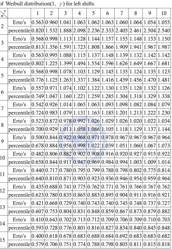
(29) Erto’s Weibull control chart when data come from Weibull process with right shifts and left shifts. The magnitude of shifts in the second column on the left is Bothe’s capability adjustments as the same as Table 7 and Table 8. We can find that the detection power is almost more than 0.5 except γ = 1 and n = 1, 2,3, 4 . For example, when data come from Weibull(1, 5) with right shift distance 1.5 σ and subgroup size n = 4 , the detection power of Erto’s Weibull control chart is 0.838>0.5. This means that the Bothe’s adjustment is inadequate and will over-adjustment the process capability. 3.6. Detection Power Comparisons. In past sections of this chapter, we have introduced three control charts for Weibull processes, and we want to know which control chart is the best powerful in control Weibull processes. Comparing the results of Table 7, Table 9, Table 11, and Table 8, Table 10, Table 12 we can find that under the same shift distance the detection power of the Erto’s Weibull control chart is the best powerful control chart. For example, when data comes from Weibull ( α = 1, γ = 5 ), and subgroup size is four, the detection power of Erto’s Weibull control chart (0.818) is better than the detection power of percentile Weibull control chart (0.699) and the detection power of bootstrap Weibull control chart(0.617). Figure 4, Figure 5, display the power curve of the percentile Weibull control chart (short-dotted line), the bootstrap Weibull control chart (long-dotted line) and the Erto’s Weibull control chart (line) when data come from Weibull ( α = 1, γ = 1(1)10 ) with right and left shifts and subgroup size are 2. We can find that the power curve of the Erto’s Weibull control chart is almost on the left of the power curve of the other two control chart except shape parameter γ > 6 and the mean shifts are small. There are other power curves with subgroup size n = 4, 6 in Appendix A. Although the detection power of the Erto’s Weibull control chart is less then the detection power of the percentile Weibull control chart in some situations, but we want to calculate the adjustment of C pk for Weibull processes, we will set the detection power is 0.5 to know the mean shifts. When the power=0.5, the mean shifts of the Erto’s Weibull control chart are shorter then the mean shifts of the percentile Weibull control chart and bootstrap Weibull control chart, so we choose the Erto’s Weibull control chart to calculate the undetected mean shift under designated power. The undetected mean shift adjustment in Table 13 and Table 14 is called AS50 which is the magnitude of shift we need to adjust based on designated detection power of the Erto’s Weibull control chart is 0.5 and process data comes from Weibull ( 1, γ ) distribution with various value of γ = 1(1)10 and the subgroup size n=2(1)15. In Table 13 and Table 14, under the same subgroup size the upper row is the AS50 which calculate by Erto’s Weibull control chart and the lower row is the AS50 which Li (2007) provided by percentile Weibull control chart. We can find that under the same shape parameter γ and subgroup size n the numbers of the upper row are smaller than the numbers of the lower row. For example, if we set γ = 5 and n=5, the adjustment of upper row is 1.020 and the lower row is 1.127. We can conclude that our result is distinctly better than the results which Li (2007) provided.. 21.

(30) Figure 4(a)-4(j). Power curve for subgroup size 2 when α=1, γ=1(1)10, k > 0 . 22.

(31) Figure 5(a)-5(j). Power curve for subgroup size 2 when α=1, γ=1(1)10, k < 0 .. 23.

(32) Why not discuss the relationship between AS 50 and scale parameter? To view the formula of skewness coefficient and kurtosis coefficient for Weibull distribution, we know scale parameter unable to affect these. So the fixed γ and subgroup size can look for the AS50 . We also don’t talk about that when the shape parameter γ < 1 because of the Equation (14). If the γ < 1 , we can’t calculate the parameter a for Erto’s Weibull control chart. Table 13. AS50 values for several subgroup sizes n and various γ values of Weibull distribution(1, γ ) for right shifts. γ 1 2 3 4 5 6 7 8 9 10 n 2 3 4 5 6 7 8 9 10 11 12 13 14 15. Erto’s. 2.513 1.954 1.703 1.582 1.495 1.446 1.378 1.336 1.321 1.288. percentile 3.611 2.492 2.009 1.767 1.632 1.536 1.470 1.424 1.387 1.359 Erto’s. 1.867 1.615 1.440 1.330 1.278 1.226 1.190 1.180 1.159 1.122. percentile 2.735 1.967 1.642 1.482 1.373 1.307 1.261 1.228 1.197 1.182 Erto’s. 1.564 1.415 1.272 1.177 1.123 1.106 1.055 1.045 1.033 1.021. percentile 2.250 1.633 1.448 1.309 1.232 1.175 1.138 1.103 1.087 1.071 Erto’s. 1.353 1.255 1.140 1.089 1.020 0.998 0.970 0.949 0.951 0.935. percentile 1.944 1.484 1.301 1.196 1.127 1.084 1.047 1.025 1.006 0.988 Erto’s. 1.203 1.146 1.068 0.992 0.951 0.918 0.905 0.881 0.873 0.859. percentile 1.716 1.343 1.201 1.104 1.043 1.009 0.981 0.960 0.942 0.932 Erto’s. 1.110 1.065 0.976 0.936 0.885 0.864 0.854 0.835 0.832 0.815. percentile 1.569 1.239 1.119 1.037 0.990 0.954 0.928 0.907 0.892 0.881 Erto’s. 1.012 0.978 0.946 0.875 0.844 0.817 0.805 0.787 0.774 0.772. percentile 1.440 1.159 1.051 0.984 0.939 0.905 0.883 0.864 0.852 0.839 Erto’s. 0.925 0.934 0.876 0.829 0.795 0.783 0.757 0.753 0.740 0.730. percentile 1.340 1.086 0.991 0.930 0.891 0.865 0.845 0.828 0.814 0.805 Erto’s. 0.859 0.890 0.839 0.801 0.753 0.751 0.727 0.711 0.703 0.703. percentile 1.251 1.031 0.943 0.889 0.853 0.828 0.811 0.797 0.784 0.773 Erto’s. 0.810 0.832 0.789 0.755 0.739 0.725 0.718 0.691 0.671 0.665. percentile 1.185 0.975 0.899 0.854 0.816 0.799 0.777 0.768 0.756 0.748 Erto’s. 0.773 0.808 0.767 0.719 0.693 0.694 0.674 0.662 0.658 0.647. percentile 1.110 0.932 0.858 0.820 0.787 0.767 0.752 0.741 0.729 0.722 Erto’s. 0.740 0.789 0.739 0.704 0.692 0.668 0.648 0.649 0.629 0.635. percentile 1.066 0.893 0.828 0.788 0.763 0.746 0.728 0.721 0.708 0.701 Erto’s. 0.715 0.759 0.714 0.680 0.665 0.645 0.638 0.627 0.601 0.608. percentile 1.021 0.861 0.801 0.762 0.737 0.723 0.709 0.696 0.688 0.684 Erto’s. 0.667 0.723 0.694 0.663 0.644 0.617 0.609 0.597 0.593 0.583. percentile 0.974 0.829 0.772 0.745 0.717 0.701 0.689 0.675 0.669 0.660 24.

(33) Table 14. AS50 values for several subgroup sizes n and various γ values of Weibull distribution(1, γ ) for left shifts. γ 1 2 3 4 5 6 7 8 9 10 n 2 3 4 5 6 7 8 9 10 11 12 13 14 15. Erto’s. 0.563 0.960 1.041 1.063 1.062 1.063 1.060 1.064 1.054 1.055. percentile 0.820 1.532 1.888 2.098 2.236 2.333 2.405 2.461 2.504 2.540 Erto’s. 0.568 0.998 1.113 1.128 1.144 1.157 1.155 1.148 1.153 1.150. percentile 0.813 1.356 1.591 1.723 1.808 1.866 1.909 1.941 1.967 1.987 Erto’s. 0.563 0.995 1.088 1.115 1.137 1.148 1.139 1.132 1.142 1.142. percentile 0.802 1.225 1.399 1.494 1.554 1.596 1.626 1.649 1.667 1.681 Erto’s. 0.568 0.998 1.078 1.103 1.129 1.145 1.135 1.124 1.135 1.123. percentile 0.776 1.125 1.263 1.337 1.384 1.416 1.439 1.456 1.470 1.481 Erto’s. 0.557 0.971 1.074 1.102 1.122 1.130 1.135 1.128 1.132 1.126. percentile 0.749 1.047 1.160 1.221 1.259 1.285 1.304 1.318 1.329 1.338 Erto’s. 0.542 0.926 1.014 1.065 1.063 1.093 1.098 1.082 1.084 1.079. percentile 0.724 0.983 1.079 1.131 1.163 1.185 1.201 1.213 1.222 1.230 Erto’s. 0.523 0.872 0.978 0.992 1.026 1.029 1.026 1.020 1.022 1.034. percentile 0.700 0.929 1.013 1.058 1.086 1.105 1.118 1.129 1.137 1.144 Erto’s. 0.500 0.844 0.922 0.968 0.971 0.978 0.967 0.967 0.967 0.964. percentile 0.678 0.884 0.958 0.998 1.022 1.039 1.051 1.060 1.067 1.073 Erto’s. 0.482 0.806 0.882 0.902 0.908 0.916 0.920 0.927 0.915 0.922. percentile 0.658 0.844 0.911 0.947 0.969 0.984 0.994 1.003 1.009 1.014 Erto’s. 0.440 0.717 0.780 0.795 0.799 0.788 0.798 0.802 0.775 0.814. percentile 0.640 0.810 0.871 0.903 0.923 0.936 0.946 0.954 0.959 0.964 Erto’s. 0.435 0.688 0.741 0.775 0.762 0.771 0.761 0.766 0.767 0.762. percentile 0.623 0.780 0.835 0.865 0.883 0.895 0.904 0.911 0.916 0.921 Erto’s. 0.421 0.668 0.729 0.740 0.743 0.740 0.745 0.748 0.737 0.727. percentile 0.607 0.753 0.804 0.831 0.848 0.859 0.867 0.873 0.879 0.882 Erto’s. 0.410 0.643 0.702 0.713 0.712 0.709 0.706 0.709 0.710 0.703. percentile 0.593 0.728 0.776 0.801 0.816 0.827 0.834 0.840 0.845 0.848 Erto’s. 0.400 0.618 0.678 0.683 0.688 0.684 0.692 0.683 0.683 0.682. percentile 0.579 0.706 0.751 0.774 0.788 0.798 0.805 0.811 0.815 0.818. 25.

(34) 4. Process Capability Adjustment for Weibull Processes 4.1 Estimator of C pk for Non-Normal Processes. The purpose of process capability indices, which are statistical measures of process capability, is based on several assumptions. Two of the most important assumption is that the process monitored is supposed to be stable and the output is approximately normal distribution. When the distribution of a process characteristic is non-normal, PCIs could often lead to erroneous and misleading interpretation of the process capability. In the recent years, several approaches the problems of PCIs for the non-normal populations have been suggested. Chen and Pearn (1997) consider come generalizations of these basic capability indices to cover non-normal distribution. Since the median is usually the preferable central value for a skewed distribution, the index C pk for non-normal processes were called C Npk were defined as:. C Npk. ⎧ ⎫ ⎪⎪ ⎪⎪ USL − M M − LSL = min ⎨ , ⎬, ⎪ ⎡ F0.99865 − F0.00135 ⎤ ⎡ F0.99865 − F0.00135 ⎤ ⎪ ⎥⎦ ⎢⎣ ⎥⎦ ⎪ ⎪⎩ ⎢⎣ 2 2 ⎭. (22). where F0.00135 is the 0.135th percentile, F0.99865 is the 99.865th percentile and M is the median. 4.2 Process Capability Adjustment of C pk for Weibull Processes. Acknowledging that a process will experience shifts in F0.50 (median) of various magnitudes and knowing that not all of these will be discovered, some allowance for them must be made when estimating outgoing quality so customers are not disappointed. Because shifts ranging in size from 0 up to AS 50σ are the likely to main undetected, a conservative approach it to assume that every missed shift it as large as AS 50 . When estimating capability, M minus AS 50σ is used to evaluate how well the process output meets the LSL and M plus AS 50σ is used for determining conformance to the USL . Both of these adjustments are incorporated into the C pk formula, now called the “dynamic” C Npk index, by making the following modifications:. dynamic C Npk. ⎧ ⎫ ⎪⎪USL − ( M + AS σ ) ( M − AS σ ) − LSL ⎪⎪ 50 50 , = min ⎨ ⎬ F F F − ⎡ 0.99865 − F0.00135 ⎤ ⎪ 0.00135 ⎤ ⎪ ⎡ 0.99865 ⎥⎦ ⎢⎣ ⎥⎦ ⎪ ⎪⎩ ⎢⎣ 2 2 ⎭. 26.

(35) ⎧ ⎫ ⎪⎪USL − M − AS σ M − AS σ − LSL ⎪⎪ 50 50 , = min ⎨ ⎬ F F F − 0.00135 ⎤ ⎡ 0.99865 − F0.00135 ⎤ ⎪ ⎪ ⎡ 0.99865 ⎢ ⎥⎦ ⎢⎣ ⎥⎦ ⎪ 2 2 ⎩⎪ ⎣ ⎭. (25). The AS50 have different results when the process distributions have right shifts or left shifts, but we can’t know what sides the processes shift to. In order to calculate the C Npk , we have to combine the upper row of Table 13 and Table 14 to get an adjustment for Weibull processes with shift distances. Since AS50 and C Npk have an inverse ratio and we would not overestimate the process capability, choose a bigger AS50 is a better choice. Table 15 shows the bigger AS50 of Table 13 and Table 14 when data come from the same parameters and we add the subgroup size to 30. For example, when data come from Weibull (1, 5) and n =5, the AS50 of the mean has right shifts is 1.0198 and the AS50 of the mean has left shifts is 1.1285, the adjustment distances for Weibull (1, 5) and n =5 are 1.1285. We conclude that the adjustment AS50 ⋅ σ ( = 1.12σ ) is required based on the detection power is 0.5 and data comes from Weibull (1, 5). By including an adjustment in this assessment for undetected shifts in median, the estimate of capability with decrease and the expected total number nonconforming parts will increase.. 27.

(36) Table 15. AS50 values for several subgroup sizes n and various γ values of Weibull distribution(1, γ ). γ 1 2 3 4 5 6 7 8 9 10 n 2. 2.513 1.954 1.703 1.582 1.495 1.446 1.378 1.336 1.321 1.288. 3. 1.867 1.615 1.440 1.330 1.278 1.226 1.190 1.180 1.159 1.150. 4. 1.564 1.415 1.272 1.177 1.137 1.148 1.139 1.132 1.142 1.142. 5. 1.353 1.255 1.140 1.103 1.129 1.145 1.135 1.124 1.135 1.123. 6. 1.203 1.146 1.074 1.102 1.122 1.130 1.135 1.128 1.132 1.126. 7. 1.110 1.065 1.014 1.065 1.063 1.093 1.098 1.082 1.084 1.079. 8. 1.012 0.978 0.978 0.992 1.026 1.029 1.026 1.020 1.022 1.034. 9. 0.925 0.934 0.922 0.968 0.971 0.978 0.967 0.967 0.967 0.964. 10. 0.859 0.890 0.882 0.902 0.908 0.916 0.920 0.927 0.915 0.922. 11. 0.810 0.832 0.789 0.795 0.799 0.788 0.798 0.802 0.775 0.814. 12. 0.773 0.808 0.767 0.775 0.762 0.771 0.761 0.766 0.767 0.762. 13. 0.740 0.789 0.739 0.740 0.743 0.740 0.745 0.748 0.737 0.727. 14. 0.715 0.759 0.714 0.713 0.712 0.709 0.706 0.709 0.710 0.703. 15. 0.667 0.723 0.694 0.683 0.688 0.684 0.692 0.683 0.683 0.682. 16. 0.650 0.707 0.669 0.667 0.667 0.681 0.663 0.674 0.665 0.656. 17. 0.630 0.672 0.644 0.650 0.656 0.637 0.650 0.647 0.646 0.656. 18. 0.600 0.663 0.628 0.626 0.640 0.635 0.629 0.631 0.637 0.629. 19. 0.580 0.645 0.606 0.626 0.614 0.621 0.611 0.609 0.611 0.612. 20. 0.564 0.626 0.596 0.597 0.600 0.601 0.599 0.593 0.603 0.588. 21. 0.549 0.604 0.583 0.587 0.582 0.591 0.582 0.580 0.586 0.586. 22. 0.549 0.596 0.568 0.588 0.564 0.579 0.572 0.567 0.569 0.567. 23. 0.532 0.574 0.558 0.559 0.572 0.564 0.557 0.557 0.552 0.552. 24. 0.512 0.562 0.542 0.553 0.548 0.551 0.547 0.544 0.549 0.546. 25. 0.500 0.554 0.536 0.548 0.540 0.534 0.546 0.529 0.532 0.534. 26. 0.489 0.547 0.528 0.527 0.528 0.516 0.519 0.524 0.526 0.522. 27. 0.473 0.532 0.512 0.514 0.520 0.511 0.518 0.509 0.517 0.509. 28. 0.468 0.528 0.508 0.512 0.508 0.508 0.496 0.503 0.500 0.494. 29. 0.457 0.524 0.505 0.493 0.492 0.492 0.492 0.495 0.493 0.492. 30. 0.447 0.517 0.498 0.482 0.494 0.486 0.484 0.479 0.480 0.472. 28.

(37) 5. An Application Adjustable speed drives (ASDs) for medium and large size motors are increasingly being adopted for the automation, transportation, and control of industrial production. However, the usage of ASDs with ac induction motors has led to the premature failure of the winding insulation. The most often reported failure occurs because of breakdown of the enameled wire insulation, and therefore, attraction of wire and motor manufacturers. It has been observed that the failure of the inter-turn insulation is more likely due to the individual or combined effect of partial discharge (PD), dielectric heating, and space charge formation. Therefore, to survive in the inverter-fed motor environment, the insulation of magnet wire must have high resistance to PD, voltage overshoots, and high frequency components that can be above the discharge inception voltage.. Figure 6. Coating layers of magnet wire insulation.. Figure 7. Pulse voltage test.. Figure 6 shows coating layers of magnet wire insulation and includes three layers (conductor, aromatic polyimide layer, PD resistant layer). Figure 7 is pulse voltage test method for wire insulation. For the insulation aging test to be representative of the voltages that result from medium voltage (1.3-7.6 kV) pulse 29.

(38) width modulated drives. For the circuit to safely and reliably operate at higher voltages it utilizes a chain of insulated gate bipolar transistor (IGBT) switches connected in series. If there is higher pulse voltage on test object, the surface of the insulation starts eroding and partial discharge, but if the pulse voltage is over USL and the surface of the insulation starts eroding, the HV DC source will shutdown. The surface roughness as measured by a scanning electron microscope. Therefore, the USL and LSL for the voltage are 7.6 kV and 1.3 kV, respectively. As shown in Table 16, a part of historical data is collected. From Figure 8 and Figure 9, it is evident to conclude the data collected from the factory are not normal distributed. The data analysis results justify that the process is significantly away from the normal distribution. By the goodness-of-fit tests, the historical data indicates that the process pretty approximates to be distributed as Weibull distribution (see Appendix B). The parameters α and γ of this Weibull process could be estimated from the historical data, giving αˆ = 4.797 and γˆ = 6 .. Figure 8. Histogram plot of the historical data.. Figure 9. Normal probability plot of the historical data. 30.

(39) Table 16. The 100 observations are collected from the historical data. 5.992 5.371. 4.413. 2.486. 4.348. 3.991. 2.892. 4.921. 4.857. 5.051. 4.508 4.695. 5.368. 4.897. 4.245. 5.273. 5.137. 4.746. 3.124. 1.783. 5.707 4.374. 5.463. 4.893. 4.145. 5.208. 4.896. 4.065. 3.507. 4.512. 5.933 5.514. 5.456. 3.107. 4.099. 5.156. 2.830. 2.288. 4.488. 4.501. 4.541 5.219. 2.514. 5.119. 4.558. 5.895. 4.497. 4.973. 4.627. 5.783. 4.537 2.876. 4.141. 3.628. 4.201. 4.390. 5.208. 5.050. 3.765. 4.686. 4.207 4.097. 4.368. 3.986. 4.528. 4.665. 5.112. 5.229. 3.807. 3.479. 4.062 3.525. 3.872. 4.223. 4.170. 4.964. 3.728. 5.360. 4.184. 4.368. 4.989 3.102. 5.470. 5.730. 4.522. 4.153. 3.308. 2.583. 4.456. 4.890. 5.269 4.507. 2.978. 3.503. 4.935. 3.896. 3.394. 4.900. 4.103. 2.379. Accordingly, it is appropriate to use this approach and we can obtain more accurate measures of the three quantiles ( F0.00135 , M , and F0.99865 ) and σ can be calculated by Equation (4). Then the dynamic C Npk index of this process can be calculated as follows:. dynamic C Npk. ⎧ ⎫ ⎪⎪USL − M − AS σ M − AS σ − LSL ⎪⎪ 50 50 = min ⎨ , ⎬ ⎪ ⎡ F0.99865 − F0.00135 ⎤ ⎡ F0.99865 − F0.00135 ⎤ ⎪ ⎥⎦ ⎢⎣ ⎥⎦ ⎪ ⎪⎩ ⎢⎣ 2 2 ⎭ ⎧ 7.6-4.51-1.145(1.02) 4.51 − 1.145(1.02) − 1.3 ⎫ =min ⎨ , ⎬ (7.08-1.29) 2 (7.08-1.29) 2 ⎩ ⎭ =min {0.66,0.71} = 0.66,. with AS50 =1.145 for n =5 from Table 15. Compared it to the value of the following conventional index : ⎧ ⎫ ⎪⎪ ⎪⎪ USL − M M − LSL , C Npk = min ⎨ ⎬ ⎪ ⎡ F0.99865 − F0.00135 ⎤ ⎡ F0.99865 − F0.00135 ⎤ ⎪ ⎥⎦ ⎢⎣ ⎥⎦ ⎪ ⎪⎩ ⎢⎣ 2 2 ⎭ =min {1.07,1.11} = 1.07,. Calculated by a traditional capability study ( the shift of process mean is not considered ), we can find that the value of the modified C Npk is much smaller. This result indicates if the process mean shifts that are not detected then unadjusted C Npk would overestimate the actual process yield which is not derisible. Our adjustment takes into account those shifts that are not detected so 31.

(40) that the practitioner would be able to keep its quality promise for this process. As the adjusted process capability drops below the desired quality level, the practitioner should stop the process because the process does not meet his present capability requirement. As the subgroup size n increases, the shift in process mean have a higher probability of detection. For example, if n =10, the AS50 would be 0.916 for Weibull (4.797, 6) from Table 15, and then the dynamic C Npk index is. dynamic C Npk. ⎧ ⎪⎪USL − M − AS σ 50 = min ⎨ F F − ⎡ 0.99865 0.135 ⎤ ⎪ ⎢ ⎥⎦ ⎪⎩ ⎣ 2. ⎫ M − AS50σ − LSL ⎪⎪ , ⎬ ⎡ F0.99865 − F0.00135 ⎤ ⎪ ⎢⎣ ⎥⎦ ⎪ 2 ⎭. ⎧ 7.6-4.51-0.916(1.02) 4.51 − 0.916(1.02) − 1.3 ⎫ =min ⎨ , ⎬ (7.08-1.29) 2 (7.08-1.29) 2 ⎩ ⎭ =min {0.74,0.79} = 0.74,. Changing n from 5 to 10 increases the dynamic C Npk index from 0.66 to 0.74, and the total number of nonconforming parts would be reduced.. 32.