Orientational Relaxation Dynamics of Liquid Water Studied by Molecular Dynamics Simulation

(1)

Orientational Relaxation Dynamics of Liquid Water Studied by Molecular Dynamics

Simulation

Yu-ling Yeh and Chung-Yuan Mou*

Department of Chemistry, National Taiwan UniVersity, Taipei, Taiwan, 106 ReceiVed: December 2, 1998; In Final Form: February 10, 1999

Orientational relaxation dynamics of water molecules in the liquid state are studied by molecular dynamics with TIP4P model. The biexponential decay of the dipolar autocorrelation function is associated with a heterogeneous distribution of local hydrogen bond patterns. The H-bond pattern was analyzed with a Voronoi polyhedra (VP) construction of the oxygen atom distributions. An asphericity parameter for VP was used to characterize the heterogeneous distribution of the local H-bond patches. The slow relaxation in the ordered region is temperature sensitive. It is associated with locally cooperative rotation around the H-bond axis. The fast (about 1 ps) relaxation, relatively temperature independent, is associated with rototranslational coupling motion of the water molecule in a disordered cage. The origin of the fast rotational relaxation comes from “interstitial molecules” coupling with the center water molecule.

I. Introduction

That liquid water can be viewed as a mixture of two or more different H-bond structures has a long and troubled history.1 For modeling liquid water, there have been two types of approaches, the continuum random network model (RNM) based on H-bond distortion2_{and various versions of mixture models.}3-5 The two-state model traditionally comes from interpreting thermodynamic properties of water,5 _{for example, density.} However, when the mixture model is inspired by fitting the thermodynamic properties, the underlying structure is uncertain. Different models can be made to reproduce the observed thermodynamic quantities by only a small adjustment of model parameters.6_{This feature makes it difficult to distinguish the} various models just from the average thermodynamic properties. Recently, the microscopic picture of liquid water became much clearer. There are many new pieces of spectroscopic evidence for the coexistence of two structures, as reflected in X-ray scattering7,8_{and Raman spectra.}9_{Bosio et al.}7_measured X-ray structural factors at pairs of temperature around maximum density to obtain isochoric temperature differentials (ITD) and identified structure rearrangement at the outer shell (distance at 3.4 Å) as the center determining factor in liquid water, in addition to the nearest H-bond neighbors. Okuhulkov et al.8 showed the strong effect of pressure on X-ray structure factors. They also proposed a mixture model that explains the change of outer shell at 3.4 Å with respect to pressure. The isosbestic points in the Raman spectrum of liquid water are also evidence for the coexisting two structures in water.9

Recently, the first dynamical spectroscopy evidence for a two-state model was found by Woutersen et al.10_{Using femtosecond} infrared pump-probe study at different regions of the O-H vibration band, they observed that the orientational relaxation of HDO in D2O consists of two time scales, with associated time constants ofτ ) 13 ps and τ ) 0.7 ps. Considering the heterogeneous distribution of relaxation times, Woutersen et al. concluded that two distinct molecular species exist in liquid water.

In viewing the recent advances in the experimental studies of liquid water structure, it would be most interesting to examine liquid water by a simulation study. In principle, computer simulations of liquid water could help to reveal the underlying heterogeneous dynamical structures. However, in most of the earlier computational work, water was viewed as a homogeneous continuous hydrogen bond network.11_{The RNM was often taken} as a viewpoint for analyzing simulation data since the advent of computer simulation partly because it is easier to analyze the configurations in this way. The problem was that there lacked local structural index to identify different local arrange-ments of the neighboring water molecules, including the outer shell at longer distance. In this paper, we show that Voronoi polyhedra (VP) structural analysis of configurations12_{can give} us a structural index to pinpoint the distinct local structures with respective orientational dynamics in liquid water.

There are many potential functions for simulation studies of water such as MCY, ST2, SPC, TIP3P, TIP4P, and their inclusions of polarization effect. The simple models consist of point charges and van der Waals interaction without intramo-lecular vibration. For the purpose of studying rotational dynam-ics and the anomalous properties of water near normal temper-ature and pressure range, TIP4P model13a_{is considered the best} choice among all the commonly used models. Recently, Jorgensen and Jenson13b_{have carried out extensive Monte Carlo} simulation using the TIP3P, SPC, and TIP4P models and they showed that the TIP4P model gives the best overall comparison with experiments. The four-site TIP4P model could yield a density maximum at 258 K, though at a somewhat lower temperature than the experimental density maximum.

The organization of this paper is as follows. In section II, we present the methods of simulation and structural analysis. Then in section III, the results of structural analysis based on Voronoi polyhedra section are discussed. Structural evidences for the heterogeneous distribution of local order are presented. The rotational relaxation dynamics of water at various local orders, as indexed by VP sections, are shown to give a biexponential decay of rotational autocorrelation function. Finally, a short conclusion is given in the last section. * Corresponding author. E-mail: cymou@ms.cc.ntu.edu.tw. Phone:

886-2-23660954. Fax: 886-2-23636359.

Downloaded by NATIONAL TAIWAN UNIV on August 11, 2009

(2)

II. Computation

We have performed the molecular dynamics simulations both in the microcanonical ensemble (NVE) at 298 K, F ) 1.0 g/cm3_, to study the structural aspects and in the isobaric-isothermal (NPT) ensemble to scan the low-temperature range at ambient pressure. The Nose-Hoover method of constant temperature and constant pressure MD algorithms14 _{with isotropic cell} fluctuations and periodic boundary conditions were employed to simulate 256 TIP4P molecules. The velocity-Verlet integra-tor is used. The position equations are deterministic and the velocity equations are solved iteratively. The equations of motion were solved with a time step of 1 fs. The cutoff distance for the Lennard-Jones interactions was set equal to half of the box length on NVE ensemble and fixed at 10 Å in NPT ensemble. The long-range Coulombic interactions were treated using the Ewald summation technique. We start the simulation by melting fcc configuration at 400 K for 10 ps and then lowering temperature to 298 K. At least 30 ps was then discarded to allow further equilibration. Because of slow equilibration in lower temperatures the last configuration at 298 K is used for the initial configuration at 265 K and so forth at each lower temperature. The density, temperature, and pressure were then monitored throughout for convergence check. The energy fluctuation was examined to ensure the equilibration. For structural analysis, we collected 5000 configurations separated by 50 time steps. The total 250 ps time length is much longer than the rotational time we are interested in this paper. In the past, distributions of water molecules were normally analyzed with the spherically averaged radial distribution (RDFs). Since local structure of water is close to that of ice, the pair correlation is highly dependent. The angle-resolved spatial distribution function (SDFs), which spans both the radial and angular coordinates of the separation vector, would be more useful. Svishchev and Kusalik15_{have applied} the SDFs to liquid water to identify the neighboring average spatial structure.

VP analysis is a particularly effective tool for clearly discriminating the topological and geometrical distribution of neighboring water molecules.12_{Here, only the coordinates of} oxygen atoms have been considered as the representative points of the water molecules. Several quantities can be measured after the Voronoi polyhedra have been built up; for example, the total volume (V), and the surface area (A) of the polyhedron. A dimensionless parameter measuring VP shape is defined as the “asphericity”,η ) A3_/36_πV2_.16_{For liquid water configurations} at normal density,η is distributed from 1.3 to 2.8.12_{For the ice} Ih structure,η is equal to 2.25. Tetrahedral-like arrangements of the nearest neighbors in liquid water will be described by a higherη value while more spherical distribution of neighbors would give a lower value ofη. Thus, η measures the anisotropic nature of the local multiple particle distribution.

III. Structure

We performed molecular dynamics on 256 water molecules using the four-site TIP4P potential.13_{A three-dimensional local} spatial density map with goo(r,Ω) ) 1.5 at T ) 298 K is plotted in Figure 1. This plot shows the most probable positions of the oxygen atoms of other water molecules surrounding the center water molecule.15_{The contours at 2.7 Å < r < 3.5 Å reflect} the distributions of the first shell oxygen atoms. At around 2.8 Å we see two distinct caps located at the hydrogen acceptor sites “A”, and a single continuous diffuse distribution at the hydrogen donor site. The continuous density distribution in the single lump in the southern hemisphere is due to a broad

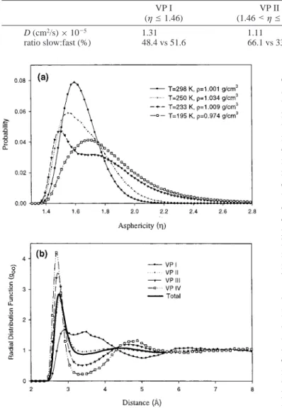
hydrogen-bonding angle distribution at the hydrogen acceptor site, including bifurcated H-bonds (“B” site). In addition, nontetrahedral “interstitial”17 _{water appears at about 3.4 Å,} which is about the distance of the van der Waals interaction of oxygen atom, and shifted by about 90°to the linear H-bond acceptors (“I” sites).15 _{Such “interstitial” water plays an} important role in the hydrogen-bond kinetics in water. It determines the rototranslation motion of water molecules in liquid state, as we will show below. Luzar and Chandler18_have used a two-state-like description of neighboring water molecules to explain their hydrogen bond breaking and formation kinetics. From Figure 2a, as the temperature decreases, the distribution ofη tends to higher value and then broadens to a bimodal form at supercooled state T ) 233 K. At this temperature, more icelike structures appear and the two structures can be roughly distinguished in the distribution. Below 220 K, the distributions ofη broaden and shift to higher values. There seems to be a rapid change around 220 K, from a thermodynamic state of low η distribution to a state of high η values. Both states have a relatively broad distribution ofη. In order to clearly see the structural and dynamical differences, we divide, somewhat arbitrarily, the whole range of asphericity into four sections in order of increasing value, from Voronoi section I to IV (VP I to VP IV). The definition of range is given in Table 1. The oxygen-oxygen pair correlation function according to different asphericity value range of the center molecule is shown in Figure 2b. An interesting feature shown in Figure 2b is that gη(r) for these four sections, show “isosbestic points” at r ) 2.9, 4.3, and 5.7 Å. One notices that the prominent peak of gηnear r ) 3.3 Å for VP I is due to interstitial water molecules. This isosbestic behavior was also found in SPC model and taken as an indication of the two coexisting states in liquid water.12_{In a} molecular dynamic study of liquid water, by analyzing the fluctuation in radial distribution, Shiratani and Sasai19_found that the individual water molecule alternately goes through two different periods: the structured period and the destructured period. The two-state structure is a dynamical one and its origin Figure 1. Oxygen atom density map around a reference water molecule at 298 K, F ) 1.0 g/cm3_{. The isosurface for g}

η(Ω,r) ) 1.5 is plotted.

The center water molecule is in the x-z plane. I, A, D, and B denote the positions of the interstitial, H-bond acceptor, H-bond donor, and bifurcated H-bond nearest neighbors, respectively.

(3)

is the heterogeneous distribution of interstitial water molecules as we will see below.

For further clarifying these two “average structures”, we show the three-dimensional contour of goo(r,Ω) for different sections. Here, we group molecules into various VP sections according to their instantaneous configurations. Figure 3, a and b, is the goo(r,Ω) map for low asphericity (the first section as VP I) and the high one (VP IV). They show very different structures. For the low asphericity section (VP I), the single lump located at hydrogen-donor sites develops a large H-bond angle distortion. The nearest-neighbor donors in VP I at site “B” (see Figure 1) prefer to align its dipole more along the dipole axis of the central molecule. The second feature in VP I is the high density of interstitial molecules. On the other hand, in VP IV, there is no H2O interstitial. The tetrahedral structure is shown clearly at the first shell. In contrast to the randomness in the angular distribution of neighboring molecules in VP I, an icelike local structure is developed for the VP IV H2O molecule.

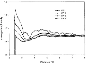
We then examine the spatial correlation of theη values. For each center molecule, we calculate the average η value of another molecule at a distance r from the center. According to their values ofη, the center molecules are again grouped into four sections as before; andηi(r), the subscript “i” indicating the Voronoi section group of the center molecule, are plotted in Figure 4. The correlation is significant. The asphericity value of the surrounding molecule is high if theη value of the center molecule is high, and vice versa. The correlations decay in a range about 6.0 Å. There is a patchlike extension of the two different structures. From the above structural analysis, we find that liquid water is composed of heterogeneous micropatches of a tetrahedral direction hydrogen-bonding pattern and a distorted hydrogen-bonding region filled with interstitials. The patchness could be the result of correlated-site percolation of hydrogen bond connectivity.20_{It has been suggested that the} icelike high-frequency sound propagation mode in water is a manifestation of collective excitation in patches of hydrogen-bonded molecules.21

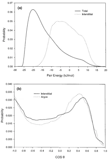
Thus, the tetrahedral icelike structure is associated with a bulkier local arrangement and the interstitial molecules are located in the region where local density is higher. And they are correlated in space to result in patchiness in arrangement. As the temperature increases, the interstitials also increase to account for the density maximum in TIP4P. This will be examined in detail in a future paper. Here we just show that interstitials are associated with higher potential energies than the normal hydrogen-bonding molecules in first neighbors. Figure 5a shows the distribution of the pair energies of the interstitials with the center molecules. It is mostly above -10 kJ/mol, rather than the -20 kJ/mol value expected for the linear H-OH hydrogen bond. The trimodal pair energy distribution with one major peak at -9 kJ/mol and other two above 0 kJ/ mol are due to different orientations of the OH relative to the center molecule. Figure 5b shows the orientation distribution of the hydrogen bond angle between OO′ and OH vector, ∠OH-O′, O′denotes the oxygen atom of the center molecule. One of the O-H bonds of the interstitial water is almost in tangential direction relative to the center. It is very close to the case where the center water molecule is replaced by an Ar atom.22_{Thus, the interstitial molecules are acting as if they were} facing a center van der Waals molecule both in energy and in orientation. The peculiar nature of water structure may be associated with the competition between the isotropic van der Waals interaction and the angle-dependent electrostatic interac-tion, both are captured in TIP4P model.

IV. Rotational Dynamics

The orientational relaxation dynamics of liquid water has been investigated recently by femtosecond nonlinear-optical polariza-tion23 _{and mid-IR pump-probe experiments.}10 _{The recent} experiment by Woutersen et al.10 _{is particularly revealing in} that they obtained a different relaxation rate (0.7 and 13 ps) by pumping at different frequencies within the inhomogeneous IR band. One should note the experimental fact that the strongly hydrogen-bonded molecules (longer wavelength absorption) can only relax through the slow process (13 ps) while the weaker TABLE 1: Diffusion Coefficient and Relaxation Behaviors at 250 K for Different Voronoi Section, the Two Rotational

Relaxation Times Being 13.0 and 1.0 ps VP I (η e 1.46) VP II (1.46 <η e 1.72) VP III (1.72 <η e 1.98) VP IV (1.98 <η) D (cm2_/s)_{× 10}-5 _1.31 _1.11 _0.95 _0.83 ratio slow:fast (%) 48.4 vs 51.6 66.1 vs 33.9 77.5 vs 22.5 85.9 vs 14.1

Figure 2. (a) Distribution of asphericity parameterη for the VP at 1 bar pressure and various temperatures. As the temperature decreases, the distribution shifts and broadens toward higher value ofη. At T ) 233 K, the distribution is bimodal reflecting two local structures. (b)

goo(r) according to the asphericity values of center reference molecule at 298 K and density F ) 1.00 g/cm3_{. The configurations are collected}

in a NVE ensemble simulation. Theη-marked goo(r) for the four sections show isosbestic points at r ) 2.9, 4.3, 5.7.η-marked goo(r)’s at other temperatures appear to be similar to the one shown here.

(4)

hydrogen-bonded molecules relax through both time scales. This effectively excludes the possibility of homogeneous distribution of the relaxation dynamics. An explanation based on a hetero-geneous distribution of local structures is thus required.

Thus it is very interesting if one could investigate the rotational dynamics of water molecules with different local structures in MD simulation. We now examine the orientational dynamics of water molecules belonging to different Voronoi sections. First, we examined the time correlation function ofη (not shown here); it consists of a stretched exponential decay, over the range of 0.5-12 ps. However, trajectories remain for relatively long time within each Voronoi section. Figure 6 shows some representative samples ofη changing with time. The large jump in the value ofη is rather infrequent. Of the six trajectories shown, only one shows extensive change inη. This is typical. Most of the trajectories stay within the same Voronoi section

in the time domain as shown in Figure 6. For the investigation of heterogeneous distribution, therefore, theη-section method is a valid index for describing different local rotational dynamics as will be shown below.

Table 1 lists the diffusion coefficients for molecules initially belonging to different Voronoi sections at 250 K, a temperature near the density maximum for the TIP4P model. Since we only classify molecules according to their instantaneous configura-tions and molecules shift between different VP secconfigura-tions during the calculation of diffusion constant, the difference of D between the VP sections in Table 1 is not large. However, molecules initially in VP I are found to have higher mobility compared to those in VP IV. This is due to the interstitial molecules existing in VP I.19

For orientational relaxation, we calculate the second-order rotational autocorrelation function of individual dipole in liquid water, which is proportional to the rotational anisotropy as

e is the unit vector of certain molecular direction, where P2(x) is the second Legendre polynomial. Czis the dipole relaxation function. We collect and average separately for molecules initially belonging to the various VP sections. The results of ln Czat T ) 250 K are presented in Figure 7. The curves of ln Cz for VP IV can be represented by a single-exponential decay with decay timeτR) 13 ps. The other curves of VP I, II, and III can be represented by biexponential decays with decay constantsτR) 13 and 1.0 ps in different ratio (Table 1). The use of VP groups help us define the local structural indexη in order to analyze the various local rotational behaviors. This is in agreement with the conclusion of the recent IR pump-probe measurement of dipole relaxation function.10_{We see the Voronoi} section with more interstitial molecules (VP I) shows faster relaxation. In a recent paper, Klein et al.24_{simulated SPC/E} water at high pressure and interstitial water was found to Figure 3. Oxygen-oxygen spatial distribution as a three-dimensional map around a center water molecule (T ) 298 K, F ) 1.00 g/cm3_{). The}

isosurfaces for gη(Ω,r) ) 2.3 (red) and 3.5 (blue) are shown for the center reference molecules which is assigned as in (a) VP I and (b) VP IV. For

VP I, the preferred closest H-bond donor is at the south pole region which can move easily between tetrahedral and pole sites and it stays for a relatively long time near the pole position to perform rotation motion. For VP IV, the close matching of red and blue isosurface indicates a localized tetrahedral arrangement of neighboring molecules.

Figure 4. Radial variation of the asphericity η(r) parameter at a distance r from the center reference molecule according to itsη-section

(T ) 298 K, F ) 1.00 g/cm3_). Ce )〈P₂[e(t)e(0)]〉

(5)

decrease the rotational correlation time. At 250 K the ratio of molecules with fast relaxation component reaches 33%, which

is close to the estimate by Marechal from ATR spectroscopy results (fast component reaches ∼35% at 0°C and∼90% at 100 °C) despite that he drew conclusions from continuous model.25_{Therefore, there are two types of molecular rotational} motion: a slow one predominating in an ordered region (VP IV) and a fast one in the disordered region(VP I). We have calculated Cz’s at temperatures from T ) 298 to 180 K, they can all be fitted by biexponential decays; the fast component is roughly temperature independent (about 1 ps) and the slow component is thermal activated but non-Arrhenius with an increasing activation energy as the temperature decreases. At 250 K, activation energy for the slow relaxation is 4.0 kcal/ mol, roughly the energy for breaking H-bond. From an Arrhenius fit of the NMR relaxation time data of liquid water26 in a small temperature range near room-temperature we find an activation energy of 4.16 kcal/mol.27

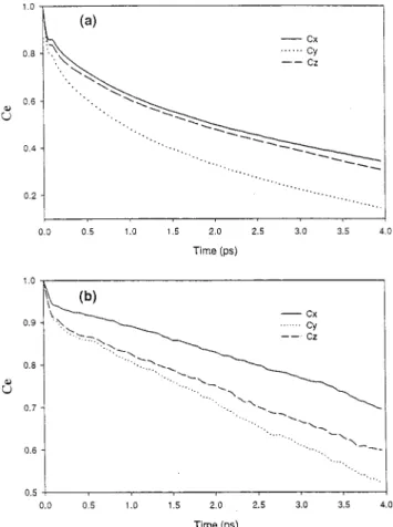
In Figure 8 we plot the Ce function (T ) 250 K) for the molecule-fixed x, y, and z axes defined in Figure 1. If there was one axis around which the rotation is predominating, the corresponding Ce function should show less decay. The relaxation in VP I (Figure 8a) shows more rotational motion around the x and z axis than the in-plane rotation. This is understandable since y-rotation will break more H-bond. The Cx and Cz curves in VP I section appear almost the same, indicating the rotation motion is more or less free around x and z. From the spatial correlation function contours in Figure 3a, we can get some idea about the minimum free energy rotation path for the center molecule. For VP I, the contour is diffuse in the south hemisphere and continuous over the south pole while the two H-bond acceptors in the north hemisphere are relatively fixed in position. This implies the oxygen atom swing motion of the center H2O is easy (with H-atoms fixed), executing an x-rotation motion in which the linear H-bond donor moves to bifurcated bond. The diffuse distribution of interstitial molecules near the H-bond acceptor favors a z-rotation of the center molecule especially if it is followed by an x-rotation and translational motion because the H-bond of an acceptor can exchange with interstitial water with a small energy change. This conclusion is reached also with visual realization of the trajectories.

Figure 9 summarizes the rotational motion of the center molecule belonging to VP I. The distribution of molecules

Figure 5. (a) Distributions of the pair energies at T ) 298 K, F ) 1.00 g/cm3_{. The bold line represents the pair energy distribution of all}

molecules, and the dashed line represents the distribution of the interstitials with the center molecules. All the curves are normalized to 1. (b) Orientational distribution of the hydrogen bond angleθ; θ is the angle between OH vector the O-O′vector, and O′is the oxygen atom of the center molecule. The bold line represents the distribution of OH vector relative to an interstitial molecule relative to the center molecule. For a comparison, the dash line represents the distribution of OH vector of neighboring water molecules relative to the center argon atom.θ is the angle between OH vector and the O-Ar vector (ref 22b). All the curves are normalized to 1.

Figure 6. Some representative samples ofη changing with time in a range of 10 ps.

Figure 7. Logarithm of the second-order rotational autocorrelation functions of the water dipole moment according to VP sections to which it belongs (T ) 250 K). Solid curves are biexponential fits to data. We add a Gaussian term to the biexponential decay to take care the initial inertial effect. Fitting function is Cz) c exp(-dt2_{/2) + a exp(-t/t}

1) + b exp(-t/t2). Bold solid curve is for the total average decay.

(6)

surrounding the center molecule is also depicted to help visualize the relative motion with respect to the neighbors. The correlated x- and z-rotation make the water molecule follow a minimum free energy path of rototranslational motion in VP I region with little activation energy. This rototranslational coupling motion has been hypothesized in previous studies on the 55 cm-1band in Raman spectrum in water.28_{Also, previously De Santis and} Rocca have examined the spatial distribution of neighboring water molecules in greater detail and find similar minimum free energy path.29

For VP IV, the decay rate of axis follows the order of Cy>

Cz> Cx(Figure 8b) and there is less translational motion while

the rotation is activated. Looking at the spatial pair distribution contour, one found while it is more concentrated than VP I, the distribution for the H-bond donor is more diffuse than the acceptor. This implies the rotation motion around the O-H axis is easier than the rotation around the O lone pair axis. After visual inspections of the trajectories, we find the rotation is indeed predominately around O-H axis (coupled with libration) and this nicely explains the decay order of Ce. If one is looking along one of the O-H bond directions, the y, z, and x axes make angles of 90°, 52°, and 38°, respectively. A rotational diffusion around an O-H direction can thus lead to the order of decay rate of Cy> Cz> Cxsince the higher the angle will lead to faster decoherence. The rotation motion around the O-H axis should be collective in nature; several neighboring similar rotations are needed to maintain the H-bonding and thus a relatively low activation energy is needed. This explains the long relaxation time that is about the same as the dielectric relaxation time that is collective in nature. Ohmine30_{has found} local collective motion associated with H-bond rearrangement dynamics; here we can locate this type of motion in the ordered region in liquid water configurations. We also note that the two-state distribution of dynamics gets more prominent in the supercooled region and may be related to the anomalous behaviors of supercooled water.31_{As the temperature is lowered,} the icelike structure gradually increases in extent, and the slow relaxation time gets longer and longer. Experimentally, this is reflected in the higher viscosity and lower diffusion constant in the supercooled region. Walrafen and Chu32_{interpreted this} by the increase of hydrogen-bonded pentagon clathrate-like structures. This needs further investigations since the relation between pentagon-ring and our structure (VP) analysis method is not clear at the present.

V. Conclusions

In conclusion, the heterogeneous distribution of the rotational relaxation can be understood by the heterogeneous distribution of “interstitial” water molecules that were found through the aid of structural index in the Voronoi polyhedra construction of configurations. The VP construction is a useful tool for recognizing local structural heterogeneity; one may want to find other more convenient local structural indexes in the future. The finding of dynamical heterogeneity is important in understanding supercooled liquid and glass.33_{There are recent simulations on} Lennard-Jones mixture,34_{high-density heterogeneity in water,}35

Figure 8. Second-order rotational autocorrelation functions of the water molecular axis x, y, z: Cx, Cy, and Cz(a) for VP I and (b) for VP IV.

Figure 9. A schematic representation of the rotational motion of the center molecule belonging to VP I. Left panel shows the swing motion along the x-axis. The right panel shows the rotational motion along the dipole axis (z-axis).

(7)

and experimental study on glass-forming liquid36_{indicating the} presence of spatially correlated dynamical heterogeneity. Our findings of the two-state rotational dynamics heterogeneity in liquid water, in explicit molecular detail, may promise to lead to a better understanding of not only this most important liquid but also the dynamics of supercooled liquid and glass.

Acknowledgment. The research is supported by the National Science Council of Taiwan (NSC 86-2113-M-002-004). We thank Professor Carmay Lim for helpful comments and Dr. Feng-yin Lee for helps in computer visualization.

References and Notes

(1) (a) Stillinger, F. H. Science 1980, 209, 451. (b) Cho, C. H.; Singh, S.; Robinson, G. W. R. Soc. Chem. Faraday Discuss. 1996, 103, 19. (c) Cho, C. H.; Singh, S.; Robinson, G. W. J. Chem. Phys. 1997, 107, 7979. (2) Sceats, M. G.; Rice, S. A. J. Chem. Phys. 1980, 72, 3236, 3248. (3) Bartell, L. S. J. Phys. Chem. B 1997, 101, 7573.

(4) Benson, S. W.; Silbert, E. D. J. Am. Chem. Soc. 1992, 114, 4269. (5) (a) Vedamuthu, M.; Singh, S.; Robinson, G. W. J. Phys. Chem. 1994, 98, 2222. (b) Vedamuthu, M.; Singh, S.; Robinson, G. W. J. Phys.

Chem. 1994, 98, 591. (c) Vedamuthu, M.; Singh, S.; Robinson, G. W. J. Phys. Chem. 1995, 99, 9263.

(6) Lee, B.; Graziano, G. J. Am. Chem. Soc. 1996, 115, 5163. (7) Bosio, L.; Chen, S. H.; Teixeira, J. Phys. ReV. 1983, A27, 1468. (8) Okhulkov, A. V.; Demianets, Yu. N.; Gorbaty, Yu. E. J. Chem. Phys. 1994, 100, 1578.

(9) Walrafen, G. E.; Hokmabadi, M. S.; Yang, W.-H. J. Chem. Phys. 1986, 85, 6964.

(10) Woutersen, S.; Emmerichs, U.; Bakker, H. J. Science 1997, 278, 658.

(11) Corongiu, G.; Clementi, E. J. Chem. Phys. 1993, 98, 2241. (12) Shih, J. P.; Sheu, S. Y.; Mou, C. Y. J. Chem. Phys. 1994, 100, 2202.

(13) (a) Jorgensen, W. L.; Chandrasekhar, J.; Madura, J. D.; Impey, R. W.; Klein, M. L. J. Chem. Phys. 1983, 79, 926. (b) Jorgensen, W. L.; Jenson, C. J. Comput. Chem. 1998, 19, 1179.

(14) Martyna, G.; Tuckerman, M. E.; Tobias, D. J.; Klein, M. L. Mol. Phys. 1996, 87, 1117.

(15) Svishchev, I. M.; Kusalik, P. G. J. Chem. Phys. 1993, 99, 3049. (16) Ruocco, G.; Sampoli, M.; Vallauri, R. J. Chem. Phys. 1992, 96, 6167.

(17) The name “interstitial” refers definitely to the position “I” in Figure 1 in the distribution of water molecules. It is related to the fifth neighboring molecule in Stanley and co-worker’s paper (Phys. ReV. Lett. 1990, 65, 3452). The name interstitial was used for the same purpose in refs 14 and 22. The quotation mark in “interstitial” is for the purpose distinguishing from the old interstitial model first proposed by Samoilov in 1965 where interstitial water molecules were thought to locate at cavity centers.

(18) (a) Luzar, A.; Chandler, D. Nature 1996, 379, 55. (b) Luzar, A.; Chandler, D. Phys. ReV. Lett. 1996, 76, 928.

(19) (a) Shiratani, E.; Sasai, M. J. Chem. Phys. 1996, 104, 7671. (b) Shiratani, E.; Sasai, M. J. Chem. Phys. 1998, 108, 3264.

(20) Stanley, H. E.; Teixeira, J. J. Chem. Phys. 1980, 73, 3404. (21) (a) Ruocco, R., et al. Nature 1996, 379, 521. (b) Sciortino, F.; Sastry, S. J. Chem. Phys. 1994, 100, 3881.

(22) (a) Geiger, A.; Rahman, A.; Stillinger, F. H. J. Chem. Phys. 1979, 70, 263. (b) Shih, J. P. Master Thesis, National Taiwan University, 1993. (23) Castner, E. W.; Chang, Y. J.; Chu, Y. C.; Walrafen, G. E. J. Chem. Phys. 1995, 102, 653.

(24) Bagchi, K.; Balasubramanian, S.; Klein, M. L. J Chem. Phys. 1997, 107, 8561.

(25) Marechal, Y. Faraday Discuss. 1996, 103, 349. (26) Nakahara, M.; Wakai C. J. Mol. Liq. 1995, 65, 149.

(27) To be sure, the temperature dependence of NMR relaxation rate is non-Arrhenius also in the larger range. From the standpoint of two-state model, this non-Arrhenius behavior is necessary.

(28) Svishchev, I. M.; Kusalik, P. G. Chem. Phys. Lett. 1993, 215, 596. (29) (a) De Santis, D.; Rocca, D. J. Chem. Phys. 1997, 107, 9559. (b) De Santis, D.; Rocca, D. J. Chem. Phys. 1997, 107, 10096.

(30) Ohmine, I. J. Phys. Chem. 1995, 99, 6767.

(31) Molecular dynamics calculation for supercooled water indicates the coexistence of low-density amorphous (LDA) and high-density amorphous (HDA) phases. The structures of LDA and HDA water may be related to the two-state water discussed in this paper (ref 18b).

(32) Walrafen, G. E.; Chu, Y. C. J. Phys. Chem. 1995, 99, 10635. (33) Ediger, M. D.; Angell, C. A.; Nagel, S. R. J. Phys. Chem. 1996, 100, 13200.

(34) Kob, W., et al. Phys. ReV. Lett. 1997, 79, 2827.

(35) Canpolat, M.; Starr, F. W.; Scala, A.; Sadr-Lahihany, M. R.; Mishima, O.; Havlin, S.; Stanley, H. E. Chem. Phys. Lett. 1998, 294, 9.

(36) Chang, I., et al. J. Non-Cryst. Solids 1994, 172, 248.