Beating the Random Walk: Intraday Seasonality and Volatility in a Developing Stock Market

Beating the Random Walk: Intraday Seasonality and Volatility

in a Developing Stock Market

Kim-Leng Goh*

Faculty of Economics and Administration, University of Malaya, Malaysia Kim-Lian Kok

Taylor’s Business School, Malaysia

Abstract

Historical prices information has not been exhaustively exploited in forecasting the 10-minute-ahead Composite Index of the Malaysian stock market. A simple model incorporating intraday seasonality can have lower forecast errors than a random walk. Improved accuracy is achieved when time-varying volatility is included in the time-of-day seasonal model for both in-sample and out-of-sample forecasts. The updating of parameter estimates of these volatility models at each new forecast origin to incorporate the latest available information leads to further improvement in forecast performance.

Key words: calendar effects; forecast; ARCH models; random walk JEL classification: C53; G14

1. Introduction

Stock market trading has broadened investment opportunities to both individual and institutional investors. Thus, the ability to accurately forecast stock market movements and the nature and behaviour of stock returns continue to be of interest to researchers and practitioners. Many early works characterized stock returns as random walks; see for example Kendall (1953), Fama (1965a, b), Granger and Morgenstern (1963), Godfrey et al. (1964), Sharma and Kennedy (1977), and Cooper (1982). The findings of these studies offer evidence that supports the efficient market hypothesis for developed stock markets.

The independence of stock returns implied by a random walk model suggests that returns are not easily predictable. With the application of new statistical tools, more recent studies posed empirical evidence against the independence of stock

Received May 24, 2005, revised May 23, 2006, accepted June 19, 2006.

*_{Corresponding Author: Faculty of Economics and Administration, University of Malaya, 50603 Kuala}

Lumpur, Malaysia. E-mail: [email protected]. The support of Bursa Malaysia in providing the data used in this study is gratefully acknowledged. We are grateful to the suggestions of the referee that led to improvement of this paper.

returns. Lo and MacKinlay (1987), Poterba and Summers (1988), Fama and French (1988), and Frennberg and Hansson (1993) found that stock returns are predictable from their mean-reverting behaviour in the long run. Contrary evidence is also found for short-run horizons. Most notable is the presence of calendar effects in stock returns which are systematically related to the time of day, the day of the week, the week of the month, the month of the year, holidays, and so forth suggesting that returns are not independent altogether. A comprehensive survey of the studies on calendar effects is provided by Sullivan et al. (2001).

The recent spate of development in autoregressive conditional heteroscedasticity (ARCH) modelling following the introduction of the idea by Engle (1982) and its subsequent generalization by Bollerslev (1986), together with the empirical support for time-varying volatility that spawned a massive literature, posed yet another challenge to the stylized random walks. Bollerslev (1987), Akgiray (1989), Nelson (1991), Tse and Tung (1992), Franses and van Dijk (1996), Walsh and Tsou (1998), and McMillan et al. (2000) are among those who used the ARCH approach to model stock market returns.

The research on the price behaviour of Bursa Malaysia, a developing stock market, went through similar developments. The stock price movements are reported to exhibit a random walk behaviour by Laurence (1986), Saw and Tan (1989), Mansor (1989), and Kok and Goh (1994a). Kok and Goh (1994b) found mean reversion for the Malaysian stock market. Significant empirical regularities pertaining to the calendar effect include the day-of-the-week effect (Davidson and Peker, 1996; Mansor, 1997) and the time-of-day effect (Chang et al., 1994; Lim, 1996; Goh and Kok, 2001). The returns are shown to display ARCH effects by Mansor (1999) and Pan et al. (1999).

When used for forecasting, a random walk suggests a naive forecast of no change. While seasonal factors arising from calendar effects and time-varying volatility are growing in importance as alternatives for explaining the behaviour of stock prices, it remains unclear whether they contain additional information content for forecasting purposes compared to a naive model. Goh and Gui (2000), for instance, found that a random walk model is difficult to beat in their assessment of the performance of various univariate and multivariate models for forecasting the Malaysian stock market sectoral indices. Their models, however, do not take into account possible calendar effects and conditional volatility. The results of Huang and Stoll (1994) and Anderson et al. (1999) show the relevance of models based on intraday seasonality and volatility for improvement of predictive power. This paper examines whether models that capture intraday seasonality patterns and time-varying volatility offer additional information compared to a random walk for forecasting the Composite Index of Bursa Malaysia. The aim is to explore if the information content of historical prices are fully exhausted and incorporated in stock prices to render the stock market efficient.

The remainder of the paper is structured as follows. Section 2 describes the data and models used together with the measures of forecast performance. Section 3 discusses the results. The findings are summarized in the concluding section.

2. Methodology

The Composite Index of Bursa Malaysia recorded at 10-minute intervals for every trading day spanning September 1998 to April 1999 is used for model estimations. The start of the sample period is after the announcement of capital controls and the fixed exchange rate regime by the government of Malaysia. Goh and Kok (2001) observed that the period since the start of the controls is more relevant for forecasting recent stock price movements in the exchange. The out-of-sample period reserved for evaluating the forecast performance of the models considered consists of 25 trading days from May 3 to June 4, 1999, and has a total of 900 observations.

The intraday 10-minute returns are given by: 1

ln( ) 100

t t t

r = p p₋ × ,

where pt is the Composite Index recorded at time t and pt−1 is the index observed 10 minutes before. The benchmark model for comparison is the random walk given as follows: 1 t t t p = p₋ +ε , (1) where _{~ . . . (0,} 2₎ t i i d N

ε σ , t= K , and T is the number of observations in the 1, ,T

sample for estimation.

Five alternative models are considered. Intraday seasonality is incorporated in the mean process of these models. The stock exchange is open for trading from Monday to Friday, and the daily trading hours are from 9:00 am to 12:30 pm and 2:30 pm to 5:00 pm. As there are 36 ten-minute intervals in a trading day, the following OLS model that captures the time-of-day effect is employed:

1 1 2 2 36 36, 1

t t t t t t

r =αD +α D + +K α D +θr− +ε , (2)

where Dit = for the i th interval and 0 otherwise, 1 i=1,2, ,36K . The term rt−1 is included in the equation to allow for a lag dependent structure. Day-of-the-week effects are not considered as the intraday seasonality does not differ significantly over different days of the week (Goh and Kok, 2001).

The remaining four models account for time-varying volatility of returns. A generalized ARCH or GARCH(1,1) model (Bollerslev, 1986) is used and the variance equation is expanded to take into consideration the systematic time-of-day pattern in volatility. According to Engle and Ng (1993), the simple first-order specification is sufficient for most empirical modelling purposes. Four dummies are included in the variance equation following Goh and Kok’s (2001) findings that volatility behaves differently at the open and close of the market compared to other times of a trading day. The model is as follows:

1 1 2 2 36 36, 1

t t t t t t

t t t u =z h 2 0 1 1 2 1 1 1 2 2 35 35, 36 36, t t t t t t t h =β +βu₋ +β h₋ +φD +φ D +φ D +φ D ,

where ut Ωt−₁~ (0, )ht , zt ~ . . . (0,1)i i d N , and Ωt−1 is the information set available at

time t−1.

Seasonality in returns can be artificially induced by the variation in equity market risks. To control the risk variation effect, the ARCH-in-mean or ARCH-M model (Engle et al., 1987) that includes the conditional standard deviation to proxy risks in the mean equation specified as follows is used:

1/ 2 1 1 2 2 36 36, 1 2 1 t t t t t t t r =αD +α D + +_K α D +θ h +θ r₋ +u (4) t t t u =z h 2 0 1 1 2 1 1 1 2 2 35 35, 36 36, t t t t t t t h =β +βu₋ +β h₋ +φD +φ D +φ D +φ D ,

Positive and negative shocks in the stock market of the same magnitude can have asymmetric impact upon stock price volatility, where downward market movements typically induce higher volatilities than upward movements. The threshold ARCH (TARCH) model (Glosten et al., 1993) is able to capture this feature. The first-order threshold model is as follows:

1 1 2 2 36 36, 1 t t t t t t r =αD +α D + +_K α D +θr₋ +u ₍₅₎ t t t u =z h 2 2 0 1 1 2 1 1 1 1 1 2 2 35 35, 36 36, t t t t t t t t t h =β +βu₋ +β h₋ +γd u_{− −} +φD +φ D +φ D +φ D ,

where dt =1 if ut <0 and dt =0 otherwise. The impact of positive news is given

by β while negative news has an impact of ₁ β γ₁+ . If γ is significantly different from zero, the impact of good and bad news is asymmetric.

Another model that allows for asymmetric impact of news is the exponential GARCH (EGARCH) model proposed by Nelson (1991). The variance equation is modified according to the EGARCH specification as stated below:

1 1 2 2 36 36, 1 t t t t t t r =αD +α D + +_K α D +θr₋ +u ₍₆₎ t t t u =z h 0 1 1 2 1 1 1 1 2 2 35 35, 36 36, ln( )ht =β +β ln(ht− )+β vt− +γvt− +φDt+φ Dt+φ D t +φ D t, where 1/ 2 t t t

v =u h . The news impact is asymmetric if γ is significantly different

from zero.

Models (2) to (6) are used to forecast one-period, or 10-minute-ahead returns. Both in-sample and out-of-sample forecasts are considered. If the forecast origin is in period i, the 10-minutes-ahead return forecast rˆ_i+1 is first obtained for each model.

accordingly. This process is repeated for the entire forecast period. For the in-sample period, i=0,1, ,_KT−1. For the out-of-sample period, i=T T, +1, ,_K T+ −s 1, where

s is the total number of out-of-sample forecasts. In the case of random walk, 1

ˆ_{i i}

p₊ = p . By comparing to the actual index, the model that has the lowest average

forecast error is deemed best. The in-sample and out-of-sample forecast performance of all the six models is assessed using the four criteria given below:

Root mean squared error (RMSE) = 1 _{( ˆ )}2

i i

i

p p

n

∑

Mean absolute deviation (MAD) = 1 _i ˆ_i i

p p

n

∑

Mean absolute percent error (MAPE) = 1 ( i ˆi) / i 100 i

p p p

n

∑

Theil inequality coefficient (Theil) =

2 2 2 1 _{( ?)} 1 1 ₁₀₀ i i i i i i i p p p p n n n ⎡ ⎤ − _⎢ + _⎥× ⎣ ⎦

∑

∑

∑

where n=T for the in-sample period and n s= for the out-of-sample period.

Two out-of-sample forecasting schemes are adopted. First is the fixed scheme where parameter estimates of the model under consideration are not updated. The same model estimated using T observations is used to forecast returns for period

1, 2, ,

T+ T+ _KT+s. Second is the recursive scheme where parameter estimates are

updated at each new forecast origin to incorporate the latest available information. Under this scheme, the model is re-estimated at every forecast origin (period i)

using T+i observations in order to forecast the return for period T+ +i 1.

The significance of the differences in forecast performance of the six models as measured by the criteria in (7) to (10) is examined using the non-parametric Friedman test. The statistic for testing the null hypothesis of no differences in the forecast performance of the six models is:

6 2 1 (1 14) 84 r i i F R = =

∑

where Ri is the total of the rank of each criterion for model i. The analysis is

performed using the different out-of-sample periods as well as the evaluation criteria as the block factor.

The MSE-F test proposed by McCracken (2004) is used to assess if the models augmented with seasonality and volatility provide additional forecast information than the random walk. The test concerns only out-of-sample forecasts. The test statistic is given by:

2 2 , , 2 , ? [ ] MSE-F ˆ rw i a i i a i i s u u u − =

∑

∑

u and uˆ2_{a i,} are one-period-ahead forecast errors for the random walk and

the augmented model, respectively. The augmented model here refers to any of the models (2) to (6) for which comparison is made against the random walk. The null hypothesis is that the random walk has a mean squared error less than or equal to the error of the augmented model, and the alternative is that the mean squared error of the augmented model is smaller. The asymptotic critical values for this test are provided by McCracken (2004).

3. Results

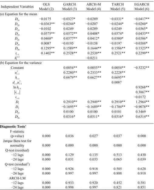
The estimated models and diagnostic checks for statistical adequacy of these models are given in Table 1. The F-statistics suggest that all the models explain movements in returns significantly. The results of the Jarque-Bera test show that the residuals are not normally distributed. To obtain consistent estimates, the quasi-maximum likelihood methods are applied to the models with time-varying volatility (see Bollerslev and Wooldridge, 1992). The returns are significantly positive at intervals 25 and 26 (30 and 40 minutes, respectively, after the open of the afternoon trading session), and the last 10 minutes before the market closes for all the models. The significance of the seasonality in the ARCH-M model implies that the seasonal pattern found in the mean process is not attributable to the variation in market risks.

The diagnostic tests indicate serious autocorrelation problem in the residuals and squared residuals of the OLS model (model (2)). The rejection of the Lagrange multiplier (LM) test for presence of the ARCH effect (Engle, 1982) also suggests that the simple OLS model is statistically inadequate. As is evident from the Q-tests, the autocorrelation problem is reduced substantially when time-varying volatility is incorporated. Since the standardized residuals and squared residuals are not autocorrelated, the specifications of models (3) through (6) are acceptable. Further, the ARCH-LM test is not significant. The 2

1

t

u− and ht−1 terms in the GARCH, ARCH-M and TARCH models ((3), (4), and (5), respectively) and the ln(ht−₁) and

1

t

v₋ terms in the EGARCH specification (model (6)) are all significant, indicating

presence of time-varying volatility. The risk-return tradeoff in the ARCH-M model is not significant for this period of study. Also, the γ coefficient in the TARCH and EGARCH models is not significantly different from zero and hence provides no evidence that the impact of news is asymmetric. The dummy variables D₁, D₂, and

36

D in the variance equation are significant in models (3) through (6), suggesting

that volatility is high in the first and last 10 minutes of the trading day. The results also indicate that the volatility at the open of the market is higher than that at the close.

Table 1. The Estimated Models for Forecasting 10-Minute-Ahead Composite Index

Independent Variables _{Model (2)} OLS _{Model (3)} GARCH ARCH-M _{Model (4) Model (5)} TARCH EGARCH _{Model (6)}

(a) Equation for the mean

16 D −0.0175 −0.0327* −0.0289 −0.0331* −0.0417** 20 D −0.0363** −0.0244* −0.0207 −0.0244* −0.0260* 24 D −0.0102 0.0249 0.0289 0.0249 0.0365* 25 D 0.0575** 0.0372** 0.0408* 0.0374* 0.0433** 26 D 0.0468* 0.0377** 0.0412* 0.0380* 0.0386* 34 D 0.0087 −0.0195 −0.0158 −0.0197 −0.0388* 36 D 0.1295** 0.1589** 0.1644** 0.1586** 0.1523** 1 t r− 0.1402** 0.2528** 0.2539** 0.2521** 0.2299** 1/ 2 t h −0.0211

(b) Equation for the variance

Constant 0.0054** 0.0055** 0.0054** −0.5232** 2 1 t u− 0.2280** 0.2333** 0.2228** 1 t h− 0.6679** 0.6627** 0.6695** 2 1 1 t t d u− − 0.0087 1 lnht− 0.9268** 1 t v− 0.3867** 1 t v− −0.0172 1 D 0.2910** 0.2949** 0.2910** 1.2964** 2 D −0.1695** −0.1689** −0.1704** −0.9078** 35 D 0.0100 0.0100 0.0101 0.3469 36 D 0.0316* 0.0311* 0.0316* 0.6314** Diagnostic Testsa F-statistic (p-value) 0.000 0.036 0.027 0.037 0.000 Jarque Bera test for

normality 0.000 0.000 0.000 0.000 0.000 Q-test (residual) −12 lags −24 lags 0.000 0.000 0.129 0.031 0.135 0.033 0.513 0.065 0.430 0.039 Q-test (residual2₎ −12 lags −24 lags 0.000 0.000 0.926 0.997 0.918 0.997 0.505 0.888 0.628 0.918 ARCH-LM −12 lags −24 lags 0.000 0.000 0.933 0.998 0.920 0.997 0.452 0.821 0.581 0.851 Notes: ** and * denote significance at 1% and 5% levels respectively. The estimated coefficients of the models are reported. Only time-of-day factors that are significant in at least one of the models are reported in the mean equation. The significance test is based on the White’s (1980) heteroscedastic-consistent standard errors for the OLS model and the quasi-maximum likelihood standard errors due to Bollerslev and Wooldridge (1992) for the other models. F-statistic is for testing the significance of the

model. Q-test (residual) and Q-test (residual2_{) refer to Q-test for significance of autocorrelation in the}

residuals and squared residuals, respectively. The standardized residuals are used for models (3) to (6).

ARCH-LM refers to the Engle (1982) LM test for presence of ARCH effects. a _{The p-values are reported}

The evaluation results of the in-sample forecast performance of these six models are shown in Table 2. For each measure, the models are ranked from 1 (lowest average forecast error) to 6 (highest average forecast error). The Friedman test indicates that the performance ranking is significantly different among the models. The average prediction errors are consistently the highest for the random walk, irrespective of the measure used. The mean rank is the lowest for EGARCH, followed by TARCH. The goodness of fit is therefore the best for the models that allow for asymmetric impact of good and bad news and is the worst for the random walk.

Table 2. Evaluation of In-Sample Forecast Performance

Measures of Forecast Errors

Model RMSE MAD MAPE Theil Mean Rank

a RW 1.68851 [6] 1.02850 [6] 0.21682 [6] 0.16602 [6] 6.0 OLS 1.65653 [1] 1.00354 [5] 0.21164 [5] 0.16288 [1] 3.0 GARCH 1.66301 [4] 0.99805 [3] 0.21075 [3] 0.16351 [4] 3.5 ARCHM 1.66335 [5] 0.99928 [4] 0.21099 [4] 0.16354 [5] 4.5 TARCH 1.66287 [3] 0.99794 [2] 0.21073 [2] 0.16350 [3] 2.5 EGARCH 1.66077 [2] 0.99749 [1] 0.21062 [1] 0.16329 [2] 1.5

Notes: Figures in brackets are the ranks of the forecast performance of each model. The rank for the model with the lowest average forecast error is 1 and for the model with the highest average forecast error is 6. RW, OLS, GARCH, ARCH-M, TARCH, and EGARCH refer to models (1) to (6) as defined in the

text. See Section 2 for definitions of the measures of forecast errors. a _{The Friedman test statistic is 14.286}

(p-value = 0.014).

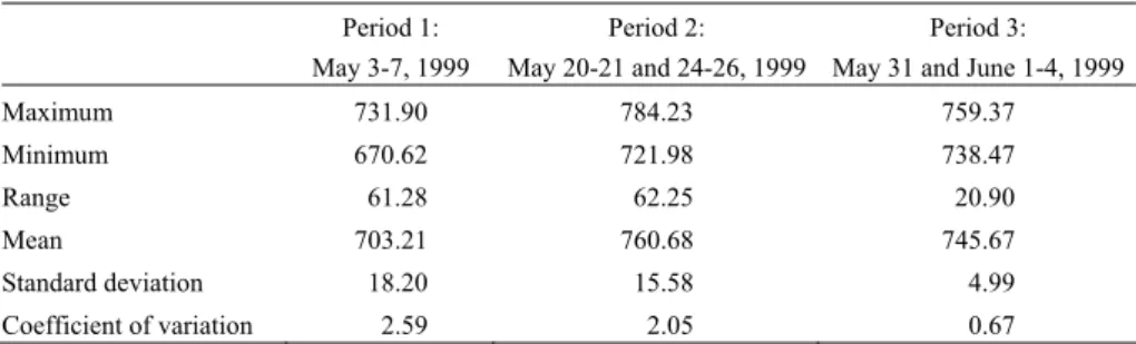
The market index at 10-minute intervals is forecasted for the 25 trading days in the out-of-sample period. In addition, the forecast performances for three sub-periods, each consisting of 5 trading days, are also analysed. The sub-sub-periods, representing different market conditions, are May 3-7 (Period 1), May 20-21 and 24-26 (Period 2), and May 31 and June 1-4 (Period 3). Table 3 provides descriptive statistics for the three sub-periods. All three sub-periods have different mean levels. The variation in the third period is lower than that of the first two periods, and price movements are within a narrower range.

Table 3. Descriptive Statistics for the Three Out-of-Sample Forecast Periods

Period 1: May 3-7, 1999

Period 2: May 20-21 and 24-26, 1999

Period 3: May 31 and June 1-4, 1999

Maximum 731.90 784.23 759.37 Minimum 670.62 721.98 738.47 Range 61.28 62.25 20.90 Mean 703.21 760.68 745.67 Standard deviation 18.20 15.58 4.99 Coefficient of variation 2.59 2.05 0.67

The out-of-sample performance measures using the fixed forecasting scheme are reported in Table 4. For the entire period, the difference between the actual and the forecast index is in the range of 1.4 to 2.0 points, or about 0.2%. The average forecast errors have about the same magnitude for Periods 1 and 2 but are much lower for Period 3. This suggests that the forecast errors are higher for the period when the market is more volatile. The models are ranked from 1 to 6 according to their forecast performance as before. The random walk has the highest or second highest average forecast error in all but two cases. In some instances, even the OLS model outperforms the random walk. The mean ranks are computed according to the measures of forecast errors and forecast periods (see Table 5). At the 10% significance level, the ranks are statistically different for each measure of forecast errors. The random walk has the highest average MAD and MAPE and the second highest RMSE and Theil inequality coefficient. The OLS model ranked close to the random walk, whereas the models capturing time-varying volatility are far superior. Generally, either the TARCH or EGARCH models have the lowest mean ranking. The evidence supporting difference in ranking of the six models is even stronger by the out-of-sample periods. Except for Period 1, the random walk has the worst mean ranking. The performance of the OLS model is just as poor. Again, the TARCH and EGARCH models are ranked either first or second for the entire period, Period 2, and Period 3.

The results of the MSE-F test in Table 6 show that all the models incorporating time-varying volatility, i.e., GARCH, ARCH-M, TARCH, and EGARCH, have significantly smaller mean squared errors than the random walk for the entire out-of-sample forecast period. The random walk also has poorer forecast accuracy than the simple OLS model and the four time-varying volatility models in Period 3. The null hypothesis of equal forecast accuracy cannot be rejected for the other two periods.

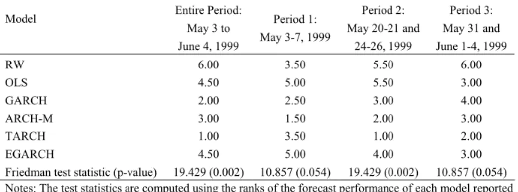
The findings are generally similar with the use of a recursive forecast scheme (see Table 7). The random walk and the OLS model rank lowest in 12 and 4 cases, respectively. The TARCH model emerges rank 1 most frequently. The EGARCH model, which ranked 4 or 5 in a few cases, does not perform as well as in the fixed forecast scheme. The differences in rank are borne out in the results of the Friedman test in Table 8. The random walk has the highest MAD and MAPE mean rank and second highest for the other two measures. The TARCH model has the best mean score across all the four measures. The performance of the EGARCH model is superseded by that of the ARCH-M model. The mean rank of the random walk is again the poorest in all the periods except Period 1. TARCH has the best performance for the entire period, Period 2, and Period 3. Again, the mean rank of ARCH-M by forecast periods is better than the mean rank of EGARCH. The results of the MSE-F test reported in Table 9 are similar to the findings for the fixed forecasting scheme. Except for OLS, all the other models with time-varying volatility have significantly lower mean squared errors compared with the random walk for the entire forecast period. In Period 3, all the models including OLS perform significantly better than the random walk.

Table 4. Out-of-Sample Forecasts with Fixed Model Scheme—Measures of Forecast Errors Model Entire Period: May 3 to June 4, 1999 Period 1: May 3-7, 1999 Period 2: May 20-21 and 24-26, 1999 Period 3: May 31 and June 1-4, 1999 RMSE RW 1.96694 [5] 2.18341 [1] 2.20333 [6] 1.48716 [6] OLS 1.96946 [6] 2.22555 [6] 2.20099 [5] 1.44458 [5] GARCH 1.95947 [2] 2.21501 [3] 2.18839 [3] 1.41793 [3] ARCH-M 1.96000 [4] 2.21493 [2] 2.19083 [4] 1.42161 [4] TARCH 1.95946 [1] 2.21575 [4] 2.18756 [1] 1.41713 [1] EGARCH 1.95953 [3] 2.21589 [5] 2.18760 [2] 1.41768 [2] MAD RW 1.40841 [6] 1.56556 [6] 1.61622 [5] 1.06811 [6] OLS 1.39941 [5] 1.56408 [5] 1.63094 [6] 1.03059 [1] GARCH 1.39778 [3] 1.56226 [2] 1.60807 [2] 1.04611 [4] ARCH-M 1.39807 [4] 1.56225 [1] 1.61328 [4] 1.04984 [5] TARCH 1.39773 [2] 1.56262 [3] 1.60717 [1] 1.04541 [3] EGARCH 1.39710 [1] 1.56326 [4] 1.60875 [3] 1.04001 [2] MAPE RW 0.19045 [6] 0.22167 [6] 0.21391 [5] 0.14320 [6] OLS 0.18921 [5] 0.22150 [5] 0.21574 [6] 0.13818 [1] GARCH 0.18897 [3] 0.22119 [1] 0.21277 [2] 0.14024 [4] ARCH-M 0.18900 [4] 0.22120 [2] 0.21346 [4] 0.14074 [5] TARCH 0.18896 [2] 0.22124 [3] 0.21266 [1] 0.14014 [3] EGARCH 0.18889 [1] 0.22134 [4] 0.21287 [3] 0.13943 [2] Theil RW 0.13269 [5] 0.15520 [1] 0.14479 [6] 0.09971 [6] OLS 0.13286 [6] 0.15819 [6] 0.14463 [5] 0.09686 [5] GARCH 0.13218 [2] 0.15744 [3] 0.14380 [3] 0.09507 [3] ARCH-M 0.13222 [4] 0.15743 [2] 0.14396 [4] 0.09531 [4] TARCH 0.13218 [1] 0.15749 [4] 0.14375 [1] 0.09502 [1] EGARCH 0.13219 [3] 0.15750 [5] 0.14375 [2] 0.09505 [2]

Notes: Figures in brackets are the ranks of the forecast performance of each model. The rank for the model with the lowest average forecast error is 1, and for the model with the highest average forecast error is 6. RW, OLS, GARCH, ARCH-M, TARCH, and EGARCH refer to models (1) to (6) as defined in the text. See Section 2 for definitions of the measures of forecast errors.

Table 5. Out-of-Sample Forecasts with Fixed Model Scheme—Results of the Friedman Test

Mean Rank by Measure of Forecast Errors Model

RMSE MAD MAPE Theil

RW 4.50 5.75 5.75 4.50 OLS 5.50 4.25 4.25 5.50 GARCH 2.75 2.75 2.50 2.625 ARCH-M 3.50 3.50 3.75 3.50 TARCH 1.75 2.25 2.25 1.875 EGARCH 3.00 2.50 2.50 3.00 Friedman test statistic (p-value) 10.143 (0.071) 10.000 (0.075) 10.571 (0.061) 9.964 (0.076)

Mean Rank by Out-of-Sample Period

Model Entire Period:

May 3 to June 4, 1999 Period 1: May 3-7, 1999 Period 2: May 20-21 and 24-26, 1999 Period 3: May 31 and June 1-4, 1999 RW 5.50 3.50 5.50 6.00 OLS 5.50 5.50 5.50 3.00 GARCH 2.375 2.25 2.50 3.50 ARCH-M 4.00 1.75 4.00 4.50 TARCH 1.625 3.50 1.00 2.00 EGARCH 2.00 4.50 2.50 2.00 Friedman test statistic (p-value) 17.590 (0.004) 11.000 (0.051) 18.857 (0.002) 13.714 (0.018)

Notes: The test statistics are computed using the ranks of the forecast performance of each model reported in Table 4.

Table 6. Out-of-Sample Forecasts with Fixed Model Scheme—Results of the MSE-F Test

Model Entire Period: May 3 to June 4, 1999 Period 1: May 3-7, 1999 Period 2: May 20-21 and 24-26, 1999 Period 3: May 31 and June 1-4, 1999 OLS −2.30 −6.75 0.38 10.77* GARCH 6.87** −5.10 2.47 18.01** ARCH-M 6.38* −5.09 2.06 16.98** TARCH 6.88** −5.22 2.60 18.23** EGARCH 6.82** −5.24 2.60 18.08**

Notes: The test statistics are computed for comparing the mean squared forecast error of each model with that of the random walk. The asymptotic 5% and 1% critical values are 4.23 and 6.60, respectively, for the entire period. The corresponding critical values are 9.18 and 13.79 for periods 1, 2, and 3 (interpolated

Table 7. Out-of-Sample Forecasts with Recursive Model Scheme—Measures of Forecast Errors Model Entire Period: May 3 to June 4, 1999 Period 1: May 3-7, 1999 Period 2: May 20-21 and 24-26, 1999 Period 3: May 31 and June 1-4, 1999 RMSE RW 1.96694 [6] 2.18341 [1] 2.20333 [6] 1.48716 [6] OLS 1.96428 [5] 2.22095 [6] 2.19878 [5] 1.43997 [5] GARCH 1.95757 [2] 2.21178 [3] 2.19159 [3] 1.41973 [3] ARCH-M 1.95812 [3] 2.21154 [2] 2.19108 [2] 1.41936 [2] TARCH 1.95716 [1] 2.21272 [4] 2.18919 [1] 1.41752 [1] EGARCH 1.95849 [4] 2.21479 [5] 2.19323 [4] 1.42017 [4] MAD RW 1.40841 [6] 1.56556 [6] 1.61622 [5] 1.06811 [6] OLS 1.39583 [4] 1.56216 [4] 1.62244 [6] 1.03036 [1] GARCH 1.39512 [2] 1.56112 [2] 1.60651 [3] 1.04402 [5] ARCH-M 1.39546 [3] 1.56045 [1] 1.60607 [2] 1.04322 [4] TARCH 1.39480 [1] 1.56161 [3] 1.60448 [1] 1.04220 [3] EGARCH 1.39606 [5] 1.56533 [5] 1.60899 [4] 1.04054 [2] MAPE RW 0.19045 [6] 0.22167 [6] 0.21391 [5] 0.14320 [6] OLS 0.18874 [4] 0.22123 [4] 0.21465 [6] 0.13814 [1] GARCH 0.18862 [2] 0.22104 [2] 0.21259 [3] 0.13996 [5] ARCH-M 0.18866 [3] 0.22094 [1] 0.21253 [2] 0.13985 [4] TARCH 0.18857 [1] 0.22111 [3] 0.21232 [1] 0.13971 [3] EGARCH 0.18876 [5] 0.22164 [5] 0.21292 [4] 0.13950 [2] Theil RW 0.13269 [6] 0.15520 [1] 0.14479 [6] 0.09971 [6] OLS 0.13251 [5] 0.15786 [6] 0.14448 [5] 0.09655 [5] GARCH 0.13205 [2] 0.15721 [3] 0.14401 [3] 0.09519 [3] ARCH-M 0.13209 [3] 0.15719 [2] 0.14398 [2] 0.09517 [2] TARCH 0.13203 [1] 0.15728 [4] 0.14386 [1] 0.09504 [1] EGARCH 0.13212 [4] 0.15742 [5] 0.14412 [4] 0.09522 [4]

Table 8. Out-of-Sample Forecasts with Recursive Model Scheme—Results of the Friedman Test

Mean Rank by Measure of Forecast Errors Model

RMSE MAD MAPE Theil

RW 4.75 5.75 5.75 4.75 OLS 5.25 3.75 3.75 5.25 GARCH 2.75 3.00 3.00 2.75 ARCH-M 2.25 2.50 2.50 2.25 TARCH 1.75 2.00 2.00 1.75 EGARCH 4.25 4.00 4.00 4.25

Friedman test statistic (p-value) 11.857 (0.037) 10.143 (0.071) 10.143 (0.071) 11.857 (0.037)

Mean Rank by Out-of-Sample Period

Model Entire Period:

May 3 to June 4, 1999 Period 1: May 3-7, 1999 Period 2: May 20-21 and 24-26, 1999 Period 3: May 31 and June 1-4, 1999 RW 6.00 3.50 5.50 6.00 OLS 4.50 5.00 5.50 3.00 GARCH 2.00 2.50 3.00 4.00 ARCH-M 3.00 1.50 2.00 3.00 TARCH 1.00 3.50 1.00 2.00 EGARCH 4.50 5.00 4.00 3.00

Friedman test statistic (p-value) 19.429 (0.002) 10.857 (0.054) 19.429 (0.002) 10.857 (0.054)

Notes: The test statistics are computed using the ranks of the forecast performance of each model reported in Table 7.

Table 9. Out-of-Sample Forecasts with Recursive Model Scheme—Results of the MSE-F Test

Model Entire Period: May 3 to June 4, 1999 Period 1: May 3-7, 1999 Period 2: May 20-21 and 24-26, 1999 Period 3: May 31 and June 1-4, 1999 OLS 2.44 −6.03 0.74 11.99* GARCH 8.63** −4.59 1.93 17.50** ARCH-M 8.12** −4.55 2.02 17.61** TARCH 9.01** −4.74 2.33 18.12** EGARCH 7.78** −5.06 1.66 17.38** Notes: The test statistics are computed for comparing the mean squared forecast error of each model with that of the random walk. The asymptotic 5% and 1% critical values are 4.26 and 6.65, respectively, for the entire period. The corresponding critical values are 9.18 and 13.80 for periods 1, 2, and 3 (interpolated from McCracken, 2004). * and ** denote significance at 5% and 1% levels.

Another issue that remains to be investigated is if inclusion of the most up-to-date information helps to improve forecast accuracy. The average forecast errors for the fixed and recursive schemes are compared using the Wilcoxon signed ranks test. The test is computed for different measures of forecast errors and also different forecast periods and the results are stated in Table 10. The recursive scheme

performs significantly better for all the forecast measures. The average forecast errors of the recursive scheme are also significantly lower for the entire out-of-sample period and Period 1. The results suggest that the updating of the forecast models as new observations become available leads to improved forecast performance.

Table 10. Wilcoxon Signed Ranks Test for Comparison of the Fixed and Recursive Forecast Schemes

Exact Test Statistic Asymptotic Test Statistic (p-value)

Measure of Forecast Errors

RMSE 60.0 −1.680 (0.093)

MAD 15.0** −3.360 (0.001)

MAPE 16.0** −3.323 (0.001)

Theil 59.5* −1.699 (0.089)

Out-of-Sample Period

Entire Period: May 3 to

June 4, 1999 0.0** −3.921 (0.000)

Period 1: May 3-7, 1999 25.0** −2.987 (0.003)

Period 2: May 20-21

and 24-26, 1999 86.0 −0.709 (0.478)

Period 3: May 31 and

June 1-4, 1999 67.0 −1.419 (0.156)

Notes: The test statistics are computed for testing if the average forecast error of the recursive scheme is smaller than that of the fixed scheme. The exact test statistic is based on the rank sum. The null hypothesis is rejected if the rank sum is less than 60 and 43 at the 5% and 1% level, respectively. * and ** denote significance at 5% and 1% levels.

We further investigate the usefulness of the forecasts for making trading decisions. For expositional purposes, a simple trading rule under the assumption of no transaction costs is considered. At each 10-minute interval, the investors make a decision to buy at the start of the interval and then sell at the end of the interval if the market is predicted to rise in that interval. The actual 10-minute return is then computed for every transaction made according to the trading decision based on each of the six models.

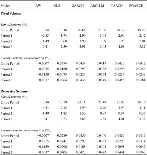
For the random walk, independent random draws from a standard normal distribution are used to predict the market movements. The sum of the actual returns and average return per transaction are reported in Table 11 for the entire out-of-sample forecast period and also for Periods 1 to 3. The results show that the returns generated from the OLS model are higher than the returns of the random walk model. Both of these models do not perform as well as the other time-varying volatility models with seasonality incorporated. The performance of all the models is better for Period 3 when the market is least volatile. Although these results hold the same for the fixed and recursive forecast schemes, the returns generated under the

recursive scheme are generally higher for the entire out-of-sample period. Inclusion of transaction costs will have the same implication for all six models. A clear indication of the results is the inferiority of the random walk for making trading decisions.

Table 11. Returns Generated under the Fixed and Recursive Forecast Schemes

Model RW OLS GARCH ARCH-M TARCH EGARCH

Fixed Scheme Sum of returns (%) Entire Period −0.34 13.36 20.68 21.06 20.37 19.26 Period 1 −0.53 1.74 2.90 3.45 2.90 2.42 Period 2 −1.49 −0.68 1.90 1.39 1.90 2.01 Period 3 0.41 2.59 3.93 3.45 4.08 3.32

Average return per transaction (%)

Entire Period −0.0007 0.0274 0.0434 0.0419 0.0430 0.0412 Period 1 −0.0055 0.0180 0.0293 0.0338 0.0293 0.0246 Period 2 −0.0159 −0.0075 0.0234 0.0164 0.0234 0.0249 Period 3 0.0037 0.0264 0.0436 0.0349 0.0458 0.0381 Recursive Scheme Sum of returns (%) Entire Period −0.34 13.79 22.11 21.49 21.82 20.16 Period 1 −0.53 2.34 2.90 2.90 2.90 3.11 Period 2 −1.49 −1.85 1.50 0.87 0.84 0.37 Period 3 0.41 3.73 3.89 3.89 4.01 3.32

Average return per transaction (%)

Entire Period −0.0007 0.0289 0.0450 0.0440 0.0450 0.0416

Period 1 −0.0055 0.0241 0.0293 0.0293 0.0293 0.0314

Period 2 −0.0159 −0.0206 0.0168 0.0102 0.0098 0.0042

Period 3 0.0037 0.0405 0.0423 0.0423 0.0441 0.0360

If a buy-and-hold strategy is followed over the individual period under consideration, the return generated at the end of each period is 9.38% for the entire-out-of-sample period, 2.76% for Period 1, −3.74% for Period 2 and −1.13% for Period 3. These figures are lower than the sum of returns generated using the models with intraday seasonality and time-varying volatility. The results suggest that these models lead to higher total returns than a simple buy-and-hold strategy, in the absence of transaction costs. However, transaction costs are practical constraints that may prevent the use of the intraday forecast strategy for investors to take advantage

of the additional predictive ability of the models. Any additional benefits may easily be outstripped by the costs when trading repeatedly at a short interval of 10 minutes. Such constraints are also noted by Huang and Stoll (1994) whose study shares similar findings.

4. Conclusion and Discussions

Ten-minute returns of the Composite Index of the Malaysian stock market are found to exhibit a significant time-of-day effect and time-varying volatility. This paper shows that even a simple OLS model incorporating only the intraday seasonality can out-perform the accuracy of a random walk for obtaining 10-minute-ahead market index forecasts. The forecast accuracy improves further with the incorporation of time-varying volatility in the model. Although the study did not find any significant asymmetry in the impact of good and bad news affecting the stock market, models that allow for such differential effects on the conditional variance exhibit better forecast performance than those that do not. The forecast errors can be reduced further if the most up-to-date information is used to estimate the model for forecasting.

In sum, significant information content is found in the intraday seasonality and volatility behaviour for forecasting the intraday stock market index. When exploited, they provide additional signals to possible future movements of the stock market compared to a random walk. As information in historical prices has not been exploited exhaustively, the Malaysian stock market is not weak form efficient. Although the Composite Index is released minute by minute to the market on a real-time basis, information is not efficiently incorporated into the prices after a lag of 10 minutes. Such information can be exploited to earn better returns than by relying purely on the random walk model. The premium is even higher if market agents update forecasts as new information becomes available.

Trading rules formulated from the forecasts of models incorporating the time-of-day component are superior those based on a pure random walk process. Although better than the random walk, transaction costs may preclude market agents from taking advantage of the predictive power of these models in reality. Further, sufficient skills are required for making such forecasts. However, the economic role of market microstructure is not irrelevant. Silber (1984) found that trades held open by scalpers in futures markets longer than 3 minutes can lead to losses. His study highlights the importance of the ability of scalpers to make decisions in extremely short time horizons.

The findings of this study suggest the occurrence of short-run regularities in the stock market and that realization of stock prices cannot be the results of chance and are thus useful for making predictions. Although the study considers only improvements in short-interval forecasts, Andersen et al. (1999) show that high-frequency intraday returns can be exploited for improving forecasts over longer horizons. Rules considered for 10-minute interval trading in this study may be of restricted use in practice because the high transaction costs incurred from frequent

trading at short time intervals may outweigh the benefits derived from exploiting the predictive power. The results, however, are indicative of the relevance and potential of the forecasts to make better trading decisions. Future work could explore the high frequency intraday regularities to identify forecast returns of longer horizons that exceed transaction costs as a trading guide.

Ederington and Lee (1993) reported that macroeconomic news announcements are responsible for most of the observed intraday volatility patterns in interest rate and foreign exchange markets. This suggests that information contained in intraday regularities can be useful for providing early signals to future stock market movements as a result of news. Signals that show the event of a large discrete drop can help avoid detrimental effects of a market crash. Future research should consider the predictive ability of models with time-of-day seasonality and volatility in datasets with large discrete jumps.

An important aspect not included in the scope of this paper is the prediction of volatility, often used as the proxy of trading risk. As improved methods to forecast volatility provide further insight on risk management, future research endeavours should investigate if the volatility forecast performance of the GARCH-type models can be improved with the incorporation of intraday seasonality and up-to-date information.

References

Akgiray, V., (1989), “Conditional Heteroscedasticity in Time Series of Stock Returns: Evidence and Forecasts,” Journal of Business, 62, 55-80.

Andersen, T. G., T. Bollerslev, and S. Lange, (1999), “Forecasting Financial Market Volatility: Sample Frequency vis-a-vis Forecast Horizon,” Journal of Empirical

Finance, 6, 457-477.

Bollerslev, T. and J. M. Wooldridge, (1992), “Quasi-Maximum Likelihood Estimation and Inference in Dynamic Models with Time Varying Covariances,” Econometric Reviews, 11, 143-172.

Bollerslev, T., (1986), “Generalized Autoregressive Conditional Heteroscedasticity,”

Journal of Econometrics, 31, 307-327.

Bollerslev, T., (1987), “A Conditional Heteroscedastic Time Series Model for Speculative Prices and Rates of Returns,” Review of Economics and Statistics, 69, 542-547.

Bollerslev, T., R. Y. Chou, and K. F. Kroner, (1992), “ARCH Modelling in Finance: A Review of the Theory and Empirical Evidence,” Journal of Econometrics, 52, 5-59.

Chang, R. P., J. K. Kang, and S. G. Rhee, (1994), “The Behaviour of Malaysian Stock Prices,” Capital Markets Review, 2(1), 15-44.

Cooper, J. C. B., (1982) “World Stock Markets: Some Random Walk Tests,”

Applied Economics, 14, 515-531.

Davidson, S. and A. Peker, (1996), “Malaysian Evidence on the Robustness of the Day-of-the-Week Effect,” Capital Markets Review, 4, 15-29.

Ederington, L. H. and J. H. Lee, (1993), “How Markets Process Information: News Releases and Volatility,” Journal of Finance, 48, 1161-1191.

Engle, R. F., D. M. Lilien, and R. P. Robins, (1987), “Estimating Time Varying Risk Premia in the Term Structure: The ARCH-M Model,” Econometrica, 55, 391-407.

Engle, R. F., (1982), “Autoregressive Conditional Heteroskedasticity with Estimates of the Variance of U.K. Inflation,” Econometrica, 50, 987-1008.

Engle, R. F. and V. K. Ng, (1993), “Measuring and Testing the Impact of News on Volatility,” Journal of Finance, 48, 1749-1778.

Fama, E. F. and K. R. French, (1988), “Permanent and Temporary Components of Stock Prices,” Journal of Political Economy, 96, 246-273.

Fama, E. F., (1965a), “The Behaviour of Stock Market Prices,” Journal of Business, 38, 34-105.

Fama, E. F., (1965b), “Tomorrow on the New York Stock Exchange,” Journal of

Business, 38, 285-299.

Franses, P. H. and D. van Dijk, (1996), “Forecasting Stock Market Volatility Using (Non-Linear) GARCH Models,” Journal of Forecasting, 15, 229-235.

Frennberg, P. and B. Hansson, (1993), “Testing the Random Walk Hypothesis on Swedish Stock Prices: 1919-1990,” Journal of Banking and Finance, 17, 175-191.

Glosten, L. R., R. Jagannathan, and D. E. Runkle, (1993), “On the Relation between the Expected Value and Volatility of the Nominal Excess Return on Stocks,”

Journal of Finance, 48, 1779-1801.

Godfrey, M., C. W. J. Granger, and O. Morgenstern, (1964), “The Random Walk Hypothesis of Stock Market Behaviour,” Kyklos, 17, 1-30.

Goh, K. L. and H. K. Gui, (2000), “Forecasting Sectoral Indices in the Kuala Lumpur Stock Exchange,” Capital Markets Review, 8, 63-88.

Goh, K. L. and K. L. Kok, (2001), “Time-of-the-Day Effect in the Malaysian Stock Market,” in Proceedings for the Third Annual Malaysian Finance Association

Workshop, Kuala Lumpur: International Islamic University Malaysia, 569-584.

Granger, C. W. J. and O. Morgenstern, (1963), “Spectral Analysis of New York Stock Market Prices,” Kyklos, 16, 1-27.

Huang, R. D. and H. R. Stoll, (1994), “Market Microstructure and Stock Return Predictions,” Review of Financial Studies, 7, 179-213.

Kendall, M. G., (1953), “The Analysis of Economic Time Series, Part I: Prices,”

Journal of the Royal Statistical Society, 96, 11-25.

Kok, K. L. and K. L. Goh, (1994a), “Weak Form Efficiency in the KLSE: New Evidence,” Capital Markets Review, 2, 45-60.

Kok, K. L. and K. L. Goh, (1994b), “Weak Form Efficiency and Mean Reversion in the Malaysian Stock Market,” Asia-Pacific Development Journal, 1, 137-152. Laurence, M. M., (1986), “Weak-Form Efficiency in the Kuala Lumpur and

Lim, E. K., (1996), “Intraday Stock Price and Volume Behaviour and Their Relationship in the Kuala Lumpur Stock Exchange,” Unpublished M.Ec dissertation, University of Malaya.

Lo, A. W. and A. C. MacKinlay, (1988), “Stock Market Prices do not Follow Random Walks: Evidence from a Simple Specification Test,” Review of

Financial Studies, 1, 41-66.

Mansor, M. I., (1989), “Share Price Behaviour on the Malaysian Stock Market: Some Empirical Evidence,” Malaysian Journal of Economic Studies, 26(1), 1-20.

Mansor, H. I., (1997), “New Evidence on Day of the Week Effect in the Malaysian Stock Market,” Capital Markets Review, 5(1), 23-33.

Mansor, H. I., (1999), “Financial Liberalisation and Stock Market Volatility in Malaysia: A GARCH Approach,” Capital Markets Review, 7, 75-86.

McCracken, M. W., (2004), “Asymptotics for Out-of-Sample Tests of Causality,” Working Paper, University of Missouri-Columbia, U.S.A.

McMillan, D., A. Speight, and O. Apgwilym, (2000), “Forecasting UK Stock Market Volatility,” Applied Financial Economics, 10, 435-448.

Nelson, D. B., (1991), “Conditional Heteroscedasticity in Asset Returns: A New Approach,” Econometrica, 59, 347-370.

Pan, M. S., Y. A. Liu, and H. J. Roth, (1999), “Common Stochastic Trends and Volatility in Asian-Pacific Equity Markets,” Global Finance Journal, 10(2), 161-172.

Poterba, J. M. and L. H. Summers, (1988), “Mean Reversion in Stock Prices: Evidence and Implications,” NBER Working Paper, No. 2343.

Saw, S. H. and K. C. Tan, (1989), “Test of Random Walk Hypothesis in the Malaysian Stock Market,” Securities Industry Review, 15, 45-50.

Sharma, J. L. and R. E. Kennedy, (1977), “A Comparative Analysis of Stock Price Behaviour on the Bombay, London and New York Stock Exchanges,” Journal

of Financial and Quantitative Analysis, 12, 391-413.

Silber, W. L., (1984), “Marketmaker Behaviour in an Auction Market: An Analysis of Scalpers in Futures Market,” Journal of Finance, 39, 937-953.

Sullivan R., A. Timmermann, and H. White, (2001), “Dangers of Data Mining: The Case of Calendar Effects in Stock Returns,” Journal of Econometrics, 105, 249-286.

Tse, Y. K. and S. H. Tung, (1992), “Forecasting Volatility in the Singapore Stock Market,” Asia Pacific Journal of Management, 9, 1-13.

Walsh, D. M. and G. Y. G. Tsou, (1998), “Forecasting Index Volatility: Sampling Interval and Non-Trading Effects,” Applied Financial Economics, 8, 477-485. White, H., (1980), “A Heteroskedasticity-Consistent Covariance Matrix and a Direct