Resource Allocation for Generic Wireless Communication Networks Considering the Effect of Multi-configuration Sectorization

全文

(1)Cover Page for 2002 International Computer Symposium (ICS2002) Workshop: Computer Networks Title of this paper: Resource Allocation for Generic Wireless Communication Networks Considering the Effect of Multi-configuration Sectorization Short abstract: In this paper, we study the resource allocation problems for channelized wireless communication networks considering generic cell configuration and obstacle shadowing effects. Resource allocation mechanisms, consist of channel assignment, power control and cell configuration design issues, are to optimize spectrum utilization of wireless systems. Furthermore, we consider both the interference-shadowing and coverage-shadowing effects due to radio propagate over topographical or morphographical obstacles. We formulate this problem as a combinatorial optimization problem, where the objective function is to minimize the total number of channels required subject to configuration, capacity, and quality of service constraints. The solution approach to the algorithm is Lagrangean relaxation. In the computational experiments, the proposed algorithm is shown to be efficient and effective. When compared with a number of sensible heuristics, the proposed algorithm achieves up to 25% improvement. Authors: Jia-An Lin, Chih-Hao Lin and Frank Yeong-Sung Lin Affiliation: Department of Information Management, National Taiwan University Postal address: No. 50, Lane 144, Keelung Rd., Sec. 4, Taipei, Taiwan, R.O.C. E-mail address: d5725001@im.ntu.edu.tw Telephone number: +886-2-2363-0231 Ext. 2812 Fax number: +886-2-2362-8423 Name of the contact author: Chih-Hao Lin Keywords: Wireless Communication Networks, Network Planning, Lagrange Relaxation, Multi-configuration Sectorization, Smart Antennas, Obstacle Effect..

(2) Resource Allocation for Generic Wireless Communication Networks Considering the Effect of Multi-configuration Sectorization Jia-An Lin, Chih-Hao Lin and Frank Yeong-Sung Lin Department of Information Management National Taiwan University Taipei, Taiwan, R.O.C. Email: d5725001@im.ntu.edu.tw. Abstract In this paper, we study the resource allocation problems for channelized wireless communication networks considering generic cell configuration and obstacle shadowing effects. Resource allocation mechanisms, consist of channel assignment, power control and cell configuration design issues, are to optimize spectrum utilization of wireless systems. For modeling generic architecture of real networks, we allow each base station can be constructed by any number of smart antennas, whose radians and transmission powers can be adjusted as needed. Furthermore, we consider both the interference-shadowing and coverage-shadowing effects due to radio propagate over topographical or morphographical obstacles. We formulate this problem as a combinatorial optimization problem, where the objective function is to minimize the total number of channels required subject to configuration, capacity, and quality of service constraints. The solution approach to the algorithm is Lagrangean relaxation. In the computational experiments, the proposed algorithm is shown to be efficient and effective. When compared with a number of sensible heuristics, the proposed algorithm achieves up to 25% improvement.. 1.

(3) I. INTRODUCTION Due to the rapid growth of wireless communication systems in the world, the scarcity of spectrum necessitates efficient resource management mechanisms. One promising technique to improve spectrum utilization and system capacity is sectorization technique, which uses smart antennas to sectorize the effect area and maximize the frequency reuse rate. That is, cellular systems are generally recognized as spectrum-efficient by increasing the frequency allocation, sectorizing the cells, and resizing the cells. Efficient spectrum utilization is one of paramount importance when designing high capacity cellular radio systems [8]. In this paper, we adopt base stations (BSs) allocation, sectorization planning, channel assignment, and power control [10] mechanisms to optimize frequency resource allocation problems. Efficient interference management aims at achieving acceptable carrier-to-interference ratio (CIR) in all active communication links and optimizing the system capacity. Traditionally, cellular network design tools usually use omni-directional or 120˚ antenna at each BS. This kind of regular architectures cannot model real network precisely [5]. In this paper, we develop a generic sectorization model to construct multi-configuration sectorization networks, which use any number of smart antennas to increase spectrum utilization. For each BS in our model, several decision variables, consist of sector number, configuration type, transmission power level, channel assignment, will be determined to optimize spectrum utilization. Furthermore, we consider the obstacle shadowing effects in the resource allocation and quality of. 2.

(4) service (QoS) assurance problems. Due to natural and man-made terrain, radio propagation is strongly influenced by different kinds of topographical and morphographical environments. In our mathematical model, the pros and cons of obstacle shadowing effects will be included. One of the advantages of obstacles is interference-shadowing effect, which can decrease the co-channel interference when obstacle located between two base stations. The disadvantage is service-shadowing effect, which will influence homing decision of MTs. We model the wireless resource allocation problem as an optimization problem, which is a non-convex integer-programming problem. To the best of our knowledge, the proposed approach is the first attempt to consider the problem with whole factors jointly and formulate it rigorously. This kind of problems is by nature highly complicated and NP-complete. Thus, we apply the Lagrange relaxation approach [6][7] and the subgradient method [9] to solve this problem. The remainder of this paper is organized as follows. Section II provides the problem description and the obstacle shadowing effects for resource allocation problems. In Section III, we introduce the solution approach, Lagrangean-based algorithm and several primal heuristics. Section IV is the computational experiments. Finally, the summary of this paper is in Section V.. II. GENERIC RESOURCE ALLOCATION PROBLEM In this section, we describe and formulate the generic resource allocation problem. We also introduce the pros and cons of obstacle shadowing effect.. 3.

(5) A. Problem Description Given limited number of available channels, candidate BS locations, traffic demand of each origin-destination (OD) pair, obstacle locations, call-blocking probability thresholds as our system parameters, we formulate this problem as a combinatorial integer-programming problem. The objective is to minimize the total number of channels required subject to capacity constraint, configuration constraint, and QoS constraint. We wish to determine (1) total number of channels required, (2) configurations of BSs, (3) transmission power levels, and (4) channel assignment policies. We define the notations for given parameters and decision variables in Table 1 and 2. Table 1: Notations of given parameters Given Parameters Notation. Descriptions. B. The set of locations for candidate BSs. F. The set of available channels. S. The set of type of antenna s mn means mth configuration and nth sector. T. The set of MTs. W. The set of OD pairs The set of configuration of BSs (In our simulation, the configuration of each BS in-. K cluding omni-directional antenna, two-sector antenna, and three-sector antenna.) D jt. Distance between BS j and MT t. 4.

(6) Upper bound on total number of channels. M N jskn. Upper bound on number of channels that can be assigned to antenna s kn in BS j. R jskn. Upper bound of radius of antenna s kn in BS j. kw. β js. User demand of OD pair w (in Erlangs) Call blocking probability of antenna s kn in BS j by user required. kn. θ ( g js , β kn. Minimum number of channels required for traffic demand g jskn such that the call js kn. Φ jskn j ' sk ' n '. ) blocking probability shall not exceed β jskn The function which is 0 if antenna s k 'n ' of BS j’ never effect antenna s kn of BS j and D −jjα' otherwise (the detail of this function is introduced in next section). G jskn. An arbitrarily large number. D jj '. Distance between BS j and j’. δ wt. Indicator function which is 1 if MT t belongs to OD pair w and 0 otherwise. µ js. Indicator function which is 1 if MT t can be served by antenna s kn in BS j and 0 othkn t. erwise. α. ρ jt. Attenuation factor (2< α <6) Indicator function which is 1 if there is no obstacle between BS j and MT t and 0 otherwise. η jj '. Indicator function which is 1 if there is no obstacle between BS j and j’ and 0 otherwise. 5.

(7) Table 2: Notations of decision variables. Decision Variables Notation. hi. Descriptions Decision variable which is 1 if channel i is installed and 0 otherwise Decision variable which is 1 if channel i is assigned to antenna s kn in BS j and 0. y jskni. otherwise r jskn. Transmission radius of antenna s kn in BS j. g jskn. Aggregate flow on antenna s kn in BS j (in Erlangs). z jskn t. Decision variable which is 1 if MT t is served by antennas s kn of BS j and 0 otherwise Decision variable which is 1 if BS j uses kth configuration. a jk. B. Problem Formulation Objective function: Z IP = min ∑ hi. (IP). i∈F. subject to:. ∑ ∑ k wδ wt z js. t∈T w∈W. kn t. ≤ g jskn. θ ( g js , β js ) ≤ ∑ y js kn. ∑ y js. i∈F. kn i. kn. i∈F. kn i. ≤ N jskn. 6. ∀j ∈ B, s kn ∈ S. (1). ∀j ∈ B, s kn ∈ S. (2). ∀j ∈ B, s kn ∈ S. (3).

(8) ∑ ∑ (rj's. 1 ) α Φ jskn j ' sk ' n ' η jj ' y j ' sk ' n 'i ≤ G jskn + ( − G jskn ) y jskni. ∀j ∈ B, s kn ∈ S , i ∈ F. (4). ∀j ∈ B, s kn ∈ S , t ∈ T. (5). ∀j ∈ B, s kn ∈ S. (6). z jskn t ≤ ρ jt µ jskn t ∑ y jskn i. ∀j ∈ B, s kn ∈ S , t ∈ T. (7). z jskn t ≤ ρ jt µ jskn t. ∀j ∈ B, s kn ∈ S , t ∈ T. (8). ∀t ∈ T. (9). ∀j ∈ B, s kn ∈ S , i ∈ F. (10). ∀j ∈ B, s kn ∈ S , i ∈ F , k ∈ K. (11). ∀j ∈ B. (12). ∀j ∈ B, i ∈ F. (13). j '∈B sk ' n ' ∈S j'≠ j. k 'n '. γ. D jt z jskn t ≤ r jskn ρ jt µ jskn t 0 ≤ r jskn ≤ R jskn. i∈F. ∑ ∑ z js j∈B skn ∈S. kn t. =1. y jskni ≤ hi y jskni ≤ a jk. ∑ a jk. =1. k ∈K. ∑ y js. skn ∈S. ∑ hi. kn i. ≤1. ≤M. (14). i∈F. hi = 0 or 1 y jskni = 0 or 1 a jk = 0 or 1 z jskn t = 0 or 1. ∀i ∈ F. (15). ∀j ∈ B, s kn ∈ S , i ∈ F. (16). ∀j ∈ B, k ∈ K. (17). ∀j ∈ B, s kn ∈ S , t ∈ T .. (18). Constraints (1) and (2) are to ensure that the number of channels assigned to each antenna is large enough to serve its slave MTs under certain call blocking probability constraint. Constraint (3) is to en-. 7.

(9) sure that the number of channels assigned to each antenna is under its capacity constraint. Constraint (4) is to ensure that for each channel, the sum of interference introduced by other co-channel BSs is less than the CIR threshold. Constraint (5) is to ensure that an antenna in the BS can only serve those MTs that are in its coverage area of effective radius. Constraint (6) is to ensure that the transmission radius of each antenna in the BS ranges between 0 and R jskn . Constraint (7) is to ensure that if an antenna is not assigned any channel, it can’t provide any service. Constraint (8) is to ensure that if an antenna does not provide service to a MT, then the decision variable z jsknt must equal to 0. Constraint (9) is to ensure that each MT must be served by exact one antenna. Constraint (10) is to ensure that we must have a channel installed before we can assign the channel to a BS. Constraint (11) is to enforce that each BS uses different kinds of antennas according to their configuration. Constraint (12) is to ensure that each BS chooses one configuration. Constraint (13) is to ensure that the antennas in the same BS cannot be assigned the same channel. Constraint (14) is to enforce the total number of total channels required is less than the number of available channels. Constraints (15)-(18) are to enforce the integer property of the decision variables.. C. Shadowing Effects of Obstacles Because transmission power is one kind of decision variables during optimization period, we introduce an over-estimate approach for channelized wireless networks to ensure QoS. For simplicity purpose, we suggest to use the maximum degree of transmission power to estimate inter-sector interference. 8.

(10) Φ jskn j 'sk 'n ' . By doing this, we can pre-calculate Φ jskn j 'sk 'n ' to reduce the uncertainty degree.. Considering sectorization effect, we propose a multi-configuration sectorization model to decide whether one antenna of BS interferes with another antennas or not. By introducing notation η jj ' , we can derive the advantage of obstacles from the interference point of view. That is denoted as interference-shadowing effect. Whereas, notation ρ jt denoted as service-shadowing effect, is the disadvantage of obstacles from the coverage point of view. To pre-calculate both these shadowing effect, we must take care of both sectorization situations of interfering and interested BSs and the locations of obstacles. For example, obstacle M is located between BS j and BS j’ in Fig. 1. Obstacle N is located between BS j and BS j’’. The cell of BS j’ is separated into two parts. One of the parts is in the shadowing area of obstacle M and the other is not. In this situation, we defined that BS j interfered with BS j’. BS j’’ is totally in the shadowing area of obstacle N will not interfere with BS j’’.. Fig. 1: Shadowing effect in Antenna Interference Model.. 9.

(11) III. SOLUTION PROCEDURE The above resource allocation problem is NP-complete. The basic approach of the solution procedure is Lagrangean relaxation method. That is, we would rather develop an efficient Lagrangean-based primal algorithm than expect to develop an optimal algorithm for large-scale NP-complete problems.. A. Lagrangean Relaxation By applying the Lagrangean relaxation approach, we relax nine complicating constraints, which are Constraints (1), (2), (4), (5), (7), (10), (11), (12) and (13). Therefore, we can formulate the Lagrange relaxation problem (LR) as follows.. Z LR (v1jskn , v 2jskn , v 3jskni , v 4jsknt , v 5jsknt , v 6jskni , v 7jsknik , v 8j , v 9ji ) = min ∑ hi + ∑. j∈B skn ∈S. i∈F. +∑. ∑ v 2js. j∈B s kn ∈S. kn. ∑ v 1js (∑ ∑ k wδ wt z js kn. t∈T w∈W. kn t. − g jskn ).   4 θ ( g jskn , β jskn ) − ∑ y jskn i  + ∑ ∑ ∑ v jskn t ( D jt z jskn t − r jskn ρ jt µ jskn t ) i∈F  j∈B skn ∈S t∈T .   1   + ∑ ∑ ∑ v 3jskni  ∑ ∑ ( rj 'sk 'n ' )α Φ jskn j 'sk 'n 'η jj ' y j 'sk 'n 'i − G jskn − ( − G jskn ) y jskni  γ j∈B skn∈S i∈F  j '∈Bsk 'n '∈S   j '≠ j  +. ∑ ∑ ∑ v 5js j∈B s kn ∈S t∈T. +∑. kn t. ( z jskn t − ρ jt µ jskn t ∑ y jskn i ) + ∑. ∑ ∑ ∑ v 7js. j∈B s kn ∈S i∈F k∈K. j∈B s kn ∈S i∈F. i∈F. kn ik. ∑ ∑ v 6js. kn i. ( y jskn i − hi ). ( y jskn i − a jk ) + ∑ v 8j ( ∑ a jk − 1) + ∑ ∑ v 9ji ( ∑ y jskni − 1) j∈B. j∈B i∈F. k∈K. (LR). skn ∈S. subject to: (3), (6), (8), (9), (14), (15), (16), (17), and (18). In this formulation, notations v 1jskn , v 2jskn , v 3jskn i , v 4jskn t , v 5jskn t , v 6jskn i , v 7jsknik , v 8j , v 9ji are non-negative Lagrange multipliers. To solve Lagrange relaxation problem (LR), we can decompose (LR) into five independent and solvable sub-problems.. 10.

(12) B. The Dual Problem and the Subgradient Method Dual Problem (D):. (. Z D1 = max Z D1 v 1jskn , v 2jskn , v 3jskni , v 4jsknt , v 5jsknt , v 6jskni , v 7jsknik , v 8j , v 9ji. ). subject to: v1jskn , v 2jskn , v 3jskni , v 4jsknt , v 5jsknt , v 6jskni , v 7jsknik , v 8j , v 9ji ≥ 0 . According to the weak Lagrange duality theorem [2], the objective of dual problem ZD is a lower bound of primal problem ZIP. We adopt the subgradient method to solve the dual problem (D) [3]. We denote a subgradient of ZD as a (|B|×(2×|S|×(1+|T|)+1+|F|×|S|×(2+|k|)))-tuple vector g. In iteration k of the. (. subgradient method, the multiplier vector π k = v 1jskn , v 2jskn ,v 3jskn i , v 4jskn t , v 5jskn t , v 6jskn i , v 7jskn ik , v 8j , v 9ji k. k. k. k. k. ). h − Z D1 (π k )) g k updated by π k +1 = π k + t k g k . The step size t k is determined by t k = δ (Z IP. is 2. h where Z IP is the primal objective function value for a heuristic solution (an upper bound on Z IP ) and δ. is a constant.. C. Getting Primal Feasible Solution When we use Lagrange relaxation and subgradient method to solve the problem, we not only get a theoretical lower bound but also get some hints that are helpful for getting primal feasible solutions purpose [6]. Owing to the complexity of the primal problem, we divide the problem into three parts by divide-and-conquer strategy and develop primal feasible algorithm, denoted as Algorithm LR. BS Configuration Subproblem When solving primal problem, we first consider to using homing decision z jskn t of each terminal to. 11.

(13) determine the BS allocation subproblem. If. ∑ ∑ z js t∈T skn ∈S. need to be allocated. Otherwise, we calculate. ∑ z js t∈T. kn t. kn t. is equal to zero, we consider this BS does not for each configuration of each BS. If. ∑ z js t∈T. kn t. is. the maximum, let this BS use kth configuration type and assign ajk to equal one. Homing Subproblem After determining allocation of the BSs, we continue to determine MTs homing subproblem. We additionally calculate two parameters, T1[j] and T2[j], for each BS. T1[j] means the number of MTs served by this BS. T2[j] means the number of MTs only served by this BS. We use these two parameters to calculate the rank of BSs in descending order of T2[j]. When the BSs have the same T2[j], we adopt descending order of T1[j] as second matter. Then, we develop the following algorithm to decide new z jsknt . According to z jsknt , we can determine the radius of each BS. Step 1. For each BS j, we calculate T2[j]×Q+T1[j] where Q is a large number to order T2[j] before T1[j]. Step 2. Arrange the BSs in descending order of the value T2[j]×Q+T1[j]. Step 3. Now, we consider only first degree of radius of each BS. If the BS is used n-sector antenna, we will consider the degree of radius of each sector at the same time. Step 4. According to the rank decided in Step 2 of BS, we assign all MTs, which are under coverage of current BS with such degree of radius and are not assigned yet, to this BS. Step 5. If any MT is not assigned, we consider next degree of radius of each BS. Repeat Step 4 until all MTs are assigned.. 12.

(14) Step 6. For each antenna in each BS, we find the maximum distance between this BS and its slave MTs. Then, we take this value to fit the degree of radius. Channel Assignment Subproblem In [4], the author took “Difficulty Degree” as the heuristics. According to the past experiment, we know DD1jskn and DD 7jskn are more suitable to simple algorithm 1 and simple algorithm 2. The detail of the two algorithms and each case are described in Section V. Because DD1jskn and DD12jskn are more suitable Lagrange relaxation based algorithm, we take DD1jskn as our primal solution to compare the results (. with. ∑ ∑ ( rjs. j '∈B −{ j } sk ' n '∈S. others.. kn. DD1jskn. is. defined. as. aggregate. interference. to. other. antennas. )α Φ j 'sk 'n ' jskn ).. IV. COMPUTATIONAL EXPERIMENTS For comparison purpose, we develop two primal heuristics to solve the same problems.. A. Primal Heuristics Heuristic with Omni-directional Antenna We assume the omni-directional antenna is only configuration in the network and develop an intuitive simple heuristic, which only consider omni-directional antenna. We determine homing decision z jsknt by adopting shortest homing policy, which homes each MT to the nearest BS, and considering the service-shadowing effect of obstacles. Then, we apply corresponding DD 1jskn to solve channel assignment subproblem. For convenience, we denote this heuristic as H1.. 13.

(15) Heuristic with Regular Three-sector Antenna This heuristic is similar to H1 except the regular configuration of 120˚ 3-sector antenna. For convenience, we denote this heuristic as H2.. B. Lagrange Relaxation Based Algorithm Algorithm LR Step 1. Read configuration file to construct MTSOs, BSs, Obstacles and MTs. Step 2. Calculate constant parameters, like θ ( g jskn , β jskn ) , Φ jskn j 'sk ' n ' , µ jsknt , ρ jt , η jj ' , and assign Lagrange relaxation improve counter to equal 20. Step 3. Initialize multipliers. Step 4. According to given multipliers, optimally solve these problems of SUB3.1, SUB3.2, SUB3.3, SUB3.4 and SUB3.5 to get the value of Zdual. Step 5. According to heuristics of Chapter 4, get the number of total channel required, the value of ZIP.. Step 6. If ZIP is smaller than ZIP*, we assign ZIP* to equal ZIP. Otherwise, we minus 1 from the improve counter. Step 7. Calculate step size and adjust Lagrange relaxation multipliers. Step 8. Iteration counter increases 1. If interaction counter is over threshold of system, stop this program. And, ZIP* is our best solution. Otherwise, Repeat step 4.. 14.

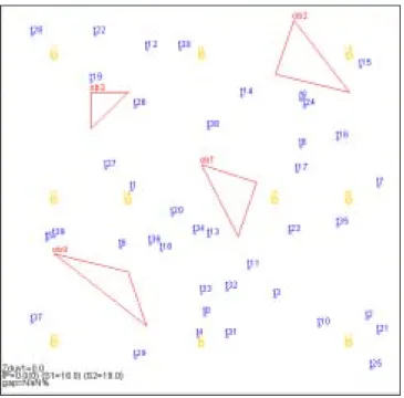
(16) C. Experiment Scenarios We randomly generate initial experiment environment as 10 BSs, 4 obstacles, 40 MTs and 20 OD-pairs and depict in Fig. 2. The feasible degrees of radius are 0.5, 1.5, 2.0, 3.0, 3.5, or 4.0 km. Traffic demands of OD-pairs are randomly generated and average 0.1 and 1.5 Erlangs for lower and higher traffic load scenario, which denote as Scenario 1 and Scenario 2, respectively.. Fig. 2: Initial locations of the BSs, Obstacles, and MTs.. D. Experiment Results At the run 0, the initial distribution is shown in Fig. 2. At other runs, we randomly generate a pair of coordinates to be the location of each MT. Each run is performed 100 iterations to get the best solution. Experiment 1 In this experiment, we apply the above three algorithms on Scenario 1 and the channel assignment is. 15.

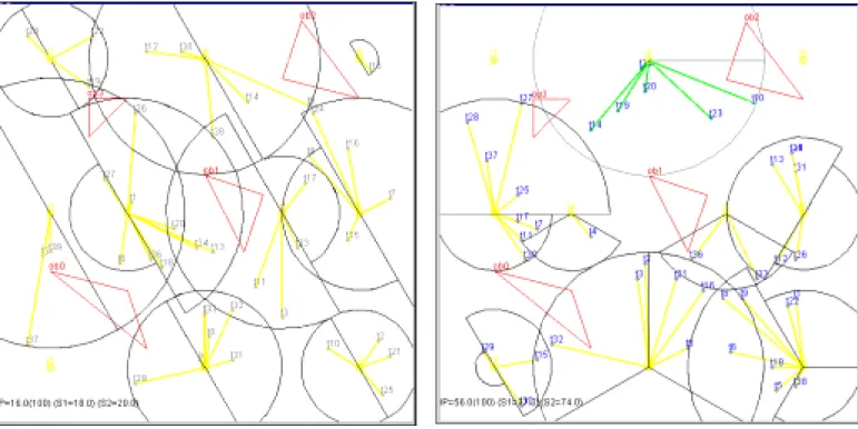
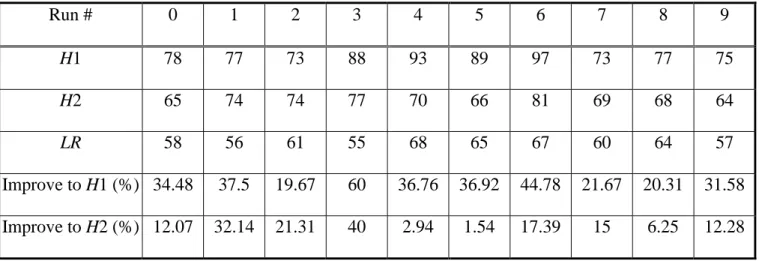
(17) decides by DD1jskn . The result of run 0 is depicted in Fig. 3 and the comparison of each run is listed in Table 3. As the results show, the proposed algorithm LR can achieve 15 % to 25% improvement against above two heuristics. Experiment 2 In Experiment 2, we use Scenario 2 as experiment network. The channel assignment is decides by DD1js. kn. . The result of run 1 is depicted in Fig. 4 and the comparison of each run is listed in Table 4. We can. observe that our proposed algorithm can achieve about 13% to 25% improvement.. Fig. 4: Result of Run 1 of Scenario 2. Fig. 3: Result of Run 0 of Scenario 1. 16.

(18) Table 3: The Result of Scenario 1 (unit: Total Channels Required) Run #. 0. 1. 2. 3. 4. 5. 6. 7. 8. 9. H1. 18. 18. 17. 20. 23. 19. 22. 18. 18. 17. H2. 20. 20. 22. 22. 24. 17. 25. 18. 22. 19. LR. 16. 17. 17. 16. 18. 16. 18. 16. 17. 15. Improve to H1 (%) 12.5. 5.88. 0. 25. 27.78. 18.75. 22.22. 1.25. 5.88. 13.33. Improve to H2 (%). 17.65. 29.41. 37.5. 33.33. 6.25. 38.89. 1.25. 29.41. 26.67. 25. Table 4: The Result of Scenario 2 (unit: Total Channels Required) Run #. 0. 1. 2. 3. 4. 5. 6. 7. 8. 9. H1. 78. 77. 73. 88. 93. 89. 97. 73. 77. 75. H2. 65. 74. 74. 77. 70. 66. 81. 69. 68. 64. LR. 58. 56. 61. 55. 68. 65. 67. 60. 64. 57. Improve to H1 (%) 34.48. 37.5. 19.67. 60. 36.76. 36.92. 44.78. 21.67. 20.31. 31.58. Improve to H2 (%) 12.07. 32.14. 21.31. 40. 2.94. 1.54. 17.39. 15. 6.25. 12.28. E. Computational Time All the experiments are performed on a Pentium 1GB PC running Microsoft Windows 2000 Server with 2 GB DRAM. The code is written in Java and is complied by Sun JDK 1.2.2. The computational time is about 90 seconds per iteration. The direct proportion between the computational time and the amount of configurations does not exist. Therefore, the computational time is the bounds of our experiments.. 17.

(19) V. SUMMARY The conclusions are presented in terms of formulation, sectorization and performance. In terms of formulation, we develop a combinatorial mathematical formulation to model the resource allocation problem for wireless communication networks with generic sectorization. At the same time, we consider not only non-uniform size cell but also non-uniform traffic demand. Specifically, we first consider the cons and pros of the obstacles shadowing effects on multi-configuration sectorization systems. Because of the complexity of this problem, we use Lagrange relaxation and subgradient method as our main methodology. In the computational experiments, the proposed algorithm is shown to be efficient and effective and can achieve up to 25% improvement on the average. In terms of sectorization, we find that sectorization is less useful when one BS needs fewer channels. By increasing the number of channels required by one BS, the advantage of sectorization is more evident. According to the experiments, in light load environment, we can say that the effect of spinning resource is more significant then the effect of reducing interference. Therefore, sectorization needs to pay the penalty in reducing the number of total channels required. However, the number of channels required by H1 is become bigger than H2 under higher traffic load. We can say that sectorization is useful in the real world to improve the spectrum efficiency as wireless traffic demands grow up rapidly. In terms of performance, our Lagrange relaxation based solution has more significant improvement than other sensible heuristics.. 18.

(20) REFERENCES [1]. G.K. Chan, “Effects of Sectorization on the Spectrum Efficiency of Cellular Radio Systems,” IEEE Transactions on Vehicular Technology, vol. 41, no. 3, pp. 217–225, August 1992.. [2]. A.M. Geoffrion, “Lagrangean Relaxation and Its Use in Integer Programming,” Math. Programming Study, vol. 2, pp. 82-114, 1974.. [3]. M. Held, P. Wolfe, and H.D. Crowder, “Validation of Subgradient Optimization,” Math. Programming, Vol. 6, pp. 62-88, 1974.. [4]. Cheng-Hon Lin, Wireless Communications Network Design and Management Considering Sectorization, Master Thesis, National Taiwan University, 2000.. [5]. C-H. Lin and F. Y-S. Lin, “Channel reassignment, augmentation and power control algorithm for wireless communications networks considering generic sectorization and channel interference,” IEEE ETS on Broadband Communications for the Internet Era, Texas, 2001.. [6]. F.Y-S. Lin, “Quasi-static Channel Assignment Algorithms for Wireless Communications Networks,” ICOIN’98, Japan, January 1998.. [7]. F.Y-S. Lin and J.L. Wang, “A Minimax Utilization Routing Algorithm in Networks with Single-path Routing,” IEEE Global Telecommunications Conference '93, vol. 2, pp. 1067-1071, 1993.. [8]. D. Saha, A. Mukherjee, and P.S. Bhattacharya, “Design of a Personal Communication Services Network (PCSN) for Optimum Location Area Size,” IEEE International Conference on Personal Wireless Communications, pp. 404-408, 1997.. [9]. D. Saha, A. Mukherjee, and S. K. Dutta, “Design of computer communication networks under link reliability constraints,” Proc. Computer, Communication, Control and Power Engineering, TENCON '93, vol. 1, pp. 188-191, 1993.. [10] J. Zander, “Performance of Optimum Transmitter Power Control in Cellular Radio Systems,” IEEE Transactions on Vehicular Technology, vol. 41, no. 1, pp. 57-62, February 1992.. 19.

(21)