Energy-Efficient Topology Control for Wireless Ad Hoc Sensor Networks

全文

(1)Energy-Efficient Topology Control for Wireless Ad Hoc Sensor Networks Yu-Chee Tseng1,† , Yen-Ning Chang2 , and Bour-Hour Tzeng1. 1. Department of Computer Science and Information Engineering 2. Department of Computer and Information Science National Chiao-Tung University Hsin-Chu, 300, Taiwan. †. E-mail: [email protected] (corresponding author) Abstract. Energy-saving is a critical issue in mobile computing. Given a set of hosts which forms a wireless ad hoc network and an initial energy for each host, this paper considers the topology control problem by tuning the transmission powers of hosts to control the structure of the network. The target topology is 1-edge-, 1-vertex-, 2-edge-, and 2-vertex-connected graphs. The goal is to maximize the lifetime of the network, i.e., the amount of time where all hosts remain alive. Two variations of the problem, where hosts’ powers can be fixed or variable during the lifetime of the network, are discussed. We show that optimal lifetimes can be obtained by using a simple minimum spanning tree construction under the fixed power assumption.. Keywords: ad hoc network, energy saving, power control, sensor network, topology control, wireless communication.. 1. Introduction. Smart sensors, which are created by tiny sensing materials combined with electrical circuits, are being proposed recently for applications such as military and environment surveillance. A wireless sensor network is established by enhancing each sensor with wireless communication capability and networking them together [5, 7]. Another similar development is the wireless ad hoc network, which is characterized by independent mobile hosts without support of fixed infrastructure [8]. Both sensor networks and ad hoc networks share the feature of multi-hop communication. Portable devices are typically powered by batteries. One major concern for almost all kinds of portable devices is how to manage the limited battery resource that constrains the life of the network. Extensive research has been devoted to ad hoc sensor networks in this direction. Using power control to reduce. 1.

(2) interference and improve throughput is addressed in [4, 16]. Topology control by tuning transmission powers is discussed in [3, 9, 14]. Power-aware routing for ad hoc networks can be found in [1, 10, 11, 12]. Both IEEE 802.11 and Bluetooth support low-power modes [2, 15]. How to design low-power modes on 802.11-based multi-hop networks is addressed in [13]. In this paper, we consider the topology control problem in an ad hoc sensor network. Topology in ad hoc networks is not a static notion since it changes as one changes the transmission powers of hosts. Given a set of hosts which forms a wireless ad hoc network and an initial energy and traffic ratio of each host, we consider the problem of determining the best transmission power of each host such that the network topology is 1-edge-, 1-vertex-, 2-edge-, or 2-vertex-connected. The goal is to maximize the lifetime of the network, i.e., the amount of time where all hosts remain alive. Two variations of the problem, where hosts’ powers can be fixed or variable throughout the lifetime of the network, are discussed. We show that optimal lifetimes can be obtained by using a simple minimum spanning tree construction under the fixed power assumption. Our work is most related to [9], where topology control algorithms to form 1-vertex and 2-vertexconnected graphs are presented. However, the initial energies of all hosts are assumed to be the same and thus this can be regarded as a special case of ours. The goal of [9] is set differently to minimize the maximal transmission power of each host in the network. Though with these differences, the approach basically also follows a minimum spanning tree construction. The result is optimal (but the resulting graph is not necessarily the same as that found by ours). So our contribution is to extend the applicability of [9] to the environment where hosts’ initial energies are not necessarily equal. The remainder of this paper is organized as follows. Section 2 formally defines the problem under consideration. Sections 3 and 4 present our solutions under the fixed and variable power constraints, respectively. Conclusions are drawn in Section 6.. 2. Problem Definition. We are given a set V of nodes on a 2-D Euclidean plane. The distance between two hosts, x and y, is denoted by dist(x, y). Since wireless communication suffers from propagation loss, the least transmission power for x and y to communicate correctly is modeled by λ(x, y) = c × dist(x, y)d , where c is a constant and d is an environment-dependent constant. The energy level of host x is a function of time and is denoted as Bx (t), where t ≥ 0 represents time. Bx (0) is a given parameter representing x’s initial energy. We adopt the following energy consumption model. Suppose x has energy Bx (t) at time t and uses power Ps to send. Then after time interval ∆t, its remaining energy becomes Bx (t + ∆t) = Bx (t) − (Ps × αx × ∆t + Pr × ∆t), where αx is the fraction of time that x transmits during ∆t and Pr is the power consumption for data reception. Note that Ps can be a variable, while Pr should remain as a constant. For example, suppose. 2.

(3) that at time t we’d like to connect two hosts x and y together using the least power λ(x, y). Then this link can sustain for the following amount of time ½ ¾ By (t) Bx (t) min , . λ(x, y) × αx + Pr λ(x, y) × αy + Pr This work considers topology control by tuning transmission powers. So the transmission power of x is also a function of time, denoted as Ps,x (t), yet to be determined. Here we assume that x’s traffic ratio αx remains as a constant throughout1 . But different hosts’ traffic ratios are not necessarily the same. By tuning transmission powers, the network topology is controllable. Specifically, for two hosts x and y, if at instant t, both Ps,x (t) and Ps,y (t) ≥ λ(x, y), we say that there is a communication link between x and y. As a result, the network topology is also a function of time, denoted as G(t) = (V, E(t)), where E(t) is the link set induced by the power setting at time t. Our goal is to maintain certain property for G(t) while keeping its lifetime as long as possible. Definition 1 Given a set of hosts V , the initial energy function Bx (0) and traffic ratio αx of each host x, and an integer k, the power adjustment problem P Ae (k) (resp., P Av (k)) is to determine the transmission power of each host such that the induced network G(t) = (V, E(t)) remains k-edge-connected (resp., kvertex-connected) during the time interval [0, T ] and T is maximized. We make three remarks below. First, a graph is k-edge-connected if the deletion of any k − 1 links in the network does not partition the network; and a graph is k-vertex-connected if the deletion of any k − 1 vertices in the network does not partition the network [6]. Under such definitions, 1-edge-connected is equivalent to 1-vertex-connected, but this is not true when k ≥ 2. Typically, vertex-connected is stronger than edge-connected. Second, if all hosts have the same initial energy, this problem degenerates to the case considered in [9]. Third, unidirectional links may exist in the network since hosts may have different transmission powers. However, only bi-directional links are included G(t) since in practice unidirectional links are difficult to use.. 3. Topology Control Under Fixed Powers. By “fixed powers”, we mean that for any host x its power function Ps,x (t) remains unchanged throughout the lifetime of the network. As a result, the topology G(t) remains unchanged too. Below, we first present an optimal solution for P Ae (1) and P Av (1), followed by one for P Ae (2) and P Av (2). Our solution to P Ae (1) and P Av (1) is similar to the typical minimum spanning tree construction in graph theory. However, here we use how long a link can sustain as the metric in the construction. Specifically, given two nodes x, y ∈ V , the lifetime of link (x, y) is defined as ½ ¾ Bx (0) By (0) t(x,y) = min , . λ(x, y) × αx + Pr λ(x, y) × αy + Pr 1 We. believe that the topology control problem would be very difficult, if not infeasible, if hosts have changing traffic. ratios. In practice, sensor network applications may impose constant traffic ratios on hosts if sensors collect data in a regular speed and certain data fusion technique is applied.. 3.

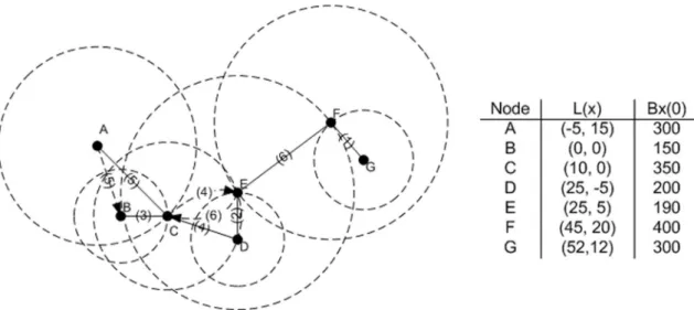
(4) A link with longer lifetime implies lower cost, and thus will be considered for inclusion earlier. The solution to P Ae (1) and P Av (1) is formally derived below. Initially, for each host x, its transmission power is set to 0, and will be increased gradually. Algorithm F P A(1). // Fixed power adjustment for P Ae (1) and P Av (1) |V |. 1. From V , construct all possible C2. node pairs. Sort these node pairs into a list (denoted as P AIR). based on their lifetimes in a descending order. 2. Construct |V | clusters of node(s) by placing each node into one separate cluster. 3. Retrieve the first node pair (x, y) from P AIR. If x and y are not in the same cluster, proceed to the next step. Otherwise, repeatedly retrieve more node pairs from P AIR, until one (x, y) such that x and y are in different clusters is found. 4. Connect link (x, y) by performing the following two steps. a) If Ps,x (t) < λ(x, y), set Ps,x (t) = λ(x, y). b) If Ps,y (t) < λ(x, y), set Ps,y (t) = λ(x, y). 5. Merge the two clusters containing x and y into one cluster. If all nodes in V are already in one cluster, terminate the algorithm; otherwise, go to step 3 and repeat. F P A(1) follows a greedy approach similar to the standard minimum spanning tree construction by using lifetimes of links as the costs. However, one interesting property is that the the resulting network is not necessarily a spanning tree — cycles may exist. The reason is that whether two nodes are connected is not determined by their link lifetime, but by how much power they use. With sufficiently large powers, links can be connected. Thus, two separate clusters may already have links (or unidirectional links). This is why we need to check nodes’ powers in step 4. Fig. 1 shows an example (here we assume that the traffic ratio is the same for all hosts). By F P A(1), we will first connect link (F, G), followed by links (D, E) and (B, C) (the order is shown by numbers in parentheses). The next link being connected is (C, D). While connecting (C, D), a side-effect directed link from C to E will appear. This is because C can reach E, but the reverse is not true. The next link being connected is (A, C), with a side-effect from A to B. The last link is (E, F ), with two side-effect links from E to B and C. Thus, we have a cycle from C to D to E. Lemma 1 The lifetime of the network constructed by F P A(1) is the lifetime of the link (x, y) which is used to merge the last two clusters in step 4. Proof. This is a natural result by the facts that P AIR is sorted in a descending order.. 2. Lemma 2 Consider the last link (x, y) being included in step 4 of FPA(1). Let C1 and C2 be the two clusters before link (x, y) is connected. The following property holds: © ª t(x,y) = max t(x0 ,y0 ) |x0 ∈ C1 , y 0 ∈ C2 .. 4.

(5) Figure 1: Example of the execution of F P A(1). Dashed arrows are side-effect links. Proof. Consider any link (x0 , y 0 ) other than (x, y) that also connects the two clusters C1 and C2 . Suppose, for contradiction, that the lifetime of (x0 , y 0 ) is longer than that of (x, y). Then in the sorted list P AIR, (x0 , y 0 ) will appear before (x, y). This implies that (x0 , y 0 ) will be examined for making connection in step 3 earlier than (x, y). Since by step 4, C1 and C2 are not connected yet when (x, y) is connected, such a link (x0 , y 0 ) can not exist. So this lemma is proved.. 2. Theorem 1 Under the fixed power constraint, the network lifetime obtained by F P A(1) is optimal for both P Ae (1) and P Av (1) problems. Proof. Consider the last link (x, y) being included in step 4 of F P A(1). Let C1 and C2 be the two clusters before link (x, y) is connected. It is clear that any algorithm must establish at least one link between C1 and C2 . Lemma 2 guarantees that (x, y) is the link that has the maximum lifetime among all links connecting C1 and C2 . So t(x,y) is an upper bound on the network lifetime that can be obtained by any algorithm. Lemma 1 states that the lifetime of the network found by FPA(1) is t(x,y) , which proves this theorem.. 2. Next, we extend our result to P Ae (2) and P Av (2) problems. The algorithm utilizes the resulting network of F P A(1) and further extend the network to 2-edge- or 2-vertex-connected. Note that although the same algorithm is used for P Ae (2) and P Av (2), the resulting networks are not necessarily the same. Algorithm F P A(2). // Fixed power adjustment for P Ae (2) and P Av (2). 1. Run F P A(1) to obtain the transmission power Ps,x (t) of each host x. Identify all 2-edge-/2-vertexconnected components in the resulting network (refer to [6] for details). |V |. 2. Again, let P AIR be the sorted list of all C2. node pairs.. 3. Retrieve the first node pair (x, y) from P AIR. If x and y are not in the same 2-edge-/2-vertexconnected component, proceed to the next step. Otherwise, repeatedly retrieve more node pairs from P AIR, until one (x, y) such that x and y are in different components is found.. 5.

(6) 4. Connect link (x, y) by performing the following two steps. a) If Ps,x (t) < λ(x, y), set Ps,x (t) = λ(x, y). b) If Ps,y (t) < λ(x, y), set Ps,y (t) = λ(x, y). 5. Identify all 2-edge-/2-vertex-connected components in the network. If only one component remains, terminate the algorithm; otherwise, go to step 3. Theorem 2 Under the fixed power constraint, the network lifetime obtained by F P A(2) is optimal for both P Ae (2) and P Av (2) problems. Proof. Before the last link, say (u, v), being added by FPA(2), there must exist at least two 2-vertex/2edge-connected components, and at least one articulation point or cut-edge. Let C1 and C2 be the two connected components where u and v are located, respectively. If any algorithm which wishes to avoid using (u, v) and has better lifetime of the network than FPA(2) does, it must construct two vertx/edgedisjoint paths between u and v without using the direct link (u, v). Furthermore, each link on these two disjoint paths must have longer lifetime than (u, v). On these two disjoint paths, there must exists at least one link, say (x, y), which is not selected by FPA(2) and is located at two distinct connected components that is able to eliminate the articulation point or cut-edge between these two components. Note that in degenerated case, it is possible that these two components are equal to C1 and C2 . However, observe that the step 3 of FPA(2) will retrieve links according to P AIR list, and the P AIR list is sorted in a descending order of link lifetime. Any link that connects different connected components and has longer lifetime than (u, v) will be selected by FPA(2) for making connection in step 3. This contradicts with our earlier assumption that (x, y) is not selected and thus this theorem is proved.. 4. 2. Topology Control under Variable Powers. F P A(1) and F P A(2) are optimal only when nodes’ transmission powers, once selected, remain unchanged. Under the variable power assumption, F P A(1) and F P A(2) are not necessarily optimal, as proved by the following counterexample. Fig. 2 shows a 4-nodes network. By running F P A(1) at time t = 0, the optimal power setting is shown in Fig. 2(a). With such setting, at time t = 0.67, if we run F P A(1) again, a new optimal setting changes to Fig. 2(b). Therefore, a variable power setting is better in this case. The detailed parameters are in Fig. 2(c). To dynamically adjust hosts’ transmission powers, we first derive a naive solution by periodically reevaluating the network topology as shown below. Algorithm V P A(k). // Variable power adjustment for P Ae (k) and P Av (k), k = 1 or 2. 1. Run F P A(k) on the current network to determine hosts’ transmission powers. 2. After a fixed interval ∆t, check hosts’ remaining energies. If none of them are dead, go back to step 1; otherwise, terminate the algorithm.. 6.

(7) Figure 2: An example of using variable powers: (a) first power setting, (b) second power setting, and (c) detailed parameters.. The above algorithm has an unspecified parameter ∆t. It can be chosen based on experience. However, it is desirable that ∆t can be determined dynamically. Below we identify some sufficient conditions which indicate that rerunning F P A(1) and F P A(2) is unnecessary. Lemma 3 Given the same set V of hosts with two different sets of initial energies for hosts, as long as the sorted link list P AIR remains unchanged, the same set of links will be connected when running F P A(1) and F P A(2). Proof. (sketched) The correctness proof for F P A(1) and F P A(2) only counts on the order of links in the list P AIR, but not on the absolute values of these links.. 2. This implies that we only need to reevaluate the network topology when the order of links in P AIR changes. Specifically, we only need to monitor each pair of neighboring links in P AIR, say (x1 , y1 ) and (x2 , y2 ), for possibility that they change their order in P AIR, if possible. Suppose that we run F P A(1) or F P A(2) at time t and (x1 , y1 ) is before (x2 , y2 ) in P AIR. Let Ps,x1 , Ps,y1 , Ps,x2 , and Ps,y2 be these hosts’ transmission powers, and Bx1 (t), By1 (t), Bx2 (t), and By2 (t) their remaining energies at time t. As time passes, we need to determine the smallest positive ∆t such that the following condition becomes true during the lifetime of the network: n min n ≤. min. Bx1 (t)−(Ps,x1 (t)αx1 +Pr )∆t By1 (t)−(Ps,y1 (t)αy1 +Pr )∆t , λ(x1 ,y1 )αx1 +Pr λ(x1 ,y1 )αy1 +Pr. Bx2 (t)−(Ps,x2 (t)αx2 +Pr )∆t By2 (t)−(Ps,y2 (t)αy2 +Pr )∆t , λ(x2 ,y2 )αx2 +Pr λ(x2 ,y2 )αy2 +Pr. o. o .. Since all factors are constants, the two components in min can be regarded as two linear functions of ∆t, i.e., they form two lines on a 2-D plane with respect to ∆t. Thus, this problem becomes a simple one of finding the earliest intersection of four lines on a 2-D plane after t and before the network lifetime expires. The above discussion gives a sufficient condition when we need to reevaluate the network topology for possibly changing hosts’ transmission powers. A further relaxation of this condition is as follows. Corollary 1 Suppose that at time t we run F P A(1) or F P A(2) to select a transmission power for each host and that at time t + ∆t the first pair of neighboring links in P AIR change their order in P AIR.. 7.

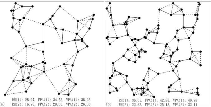
(8) If none of these two links are chosen for making connection in the corresponding algorithm (in step 4), then rerunning F P A(1) or F P A(2) at time t + ∆t + ² will result in the same power setting as that in time t, where ² is an infinitely small value. Intuitively, a link in P AIR that is not chosen for making connection does not contribute to the connectivity of the network. As a result, two such links which change their order in P AIR will not result in different power setting.. 5. Simulation Results. To evaluate the performance of the proposed F P A(i) and V P A(i) schemes, i = 1, 2, we have developed a simulator to observe the power consumption factor. A number of randomly generated hosts are placed in a 10×10 plane on real domain, where each unit is 1 kilometer. The electricity in each host is randomly selected between 80 to 120 units with a uniform distribution. A time unit is of length one hour. The power-consumption constant c is set to 1. As a result, a pair of hosts with electricity 100 units distanced by 1 km has a lifetime of 100 hours, while such hosts distanced by 10 km has a lifetime of 1 hour. Note that the absolute values in the above setting are in fact nonessential since we will focus on the relative benefits that can be obtained by the proposed schemes. Fig. 5 shows two simulation scenarios with 50 and 100 randomly generated hosts. The solid lines represent the network constructed by algorithm F P A(1), while the dashed lines represent the additional links added by F P A(2). The networks that will be constructed by [9] are not shown, but the obtained network lifetimes are denoted by “RH” in the figure. The networks that will be obtained by V P A(1) and V P A(2) are not shown either since the resulting topologies will in fact change by time. The numbers on the bottom of each subfigure represent the network lifetimes obtained by different algorithms. As can be seen, significant improvement can be obtained, both from RH scheme to FPA scheme and from FPA scheme to VPA scheme. Finally, we remark that we have used the same simulator to observe the effect of factors, such as initial battery levels and host density, on network lifetimes. However, we found that the results vary a lot and there is not conclusive trends. We believe that the reason is because the performance highly depends on the distribution of the hosts on the 2D plane and the number of possible host distributions could be extremely large, making it very difficult to see a clear trend.. 6. Conclusions. To the best of our knowledge, this work is the first one which addresses ad hoc networks’ topology control problem by taking into account hosts’ remaining energies. Algorithms for constructing 1-edge-, 1-vertex-, 2-edge-, and 2-vertex-connected networks are presented. While the basic approach is minimum spanning tree construction, the result is optimal under the fixed power model. So our contribution is on extending the applicability of [9] to the case where hosts’ initial energies can differ. Under the variable. 8.

(9) Figure 3: Comparison of network lifetimes obtained by different schemes: (a) 50 nodes and (b) 100 nodes. Solid links are obtained by F P A(1), while dashed links are extra links added by F P A(2).. power assumption, several sufficient conditions are proposed to reflect when reevaluating the network topology may be necessary. Under the fixed power model, [9] discusses how to reduce individual hosts’ powers (called PerNodeMinimize). This can remove some side-effect links, but the network lifetime cannot be improved. The result can be applied to our work under the variable power model since side-effect links may potentially become critical links in the future. Distributed topology control is discussed in [9]. While this is desirable, extending our schemes to distributed ones will make less sense since determining a graph’s connectivity needs global information.. References [1] J.-H. Chang and L. Tassiulas. Energy Conserving Routing in Wireless Ad-hoc Networks. In INFOCOM, 2000. [2] J. C. Haartsen and S. Mattisson. Bluetooth - A New Low-Power Radio Interface Providing ShortRange Connectivity. Proceedings of the IEEE, October 2000. [3] L. Hu. Topology Control for Multihop Packet Radio Networks. IEEE Transactions on Communications, 41:1474–1481, October, 1993. [4] C.-F. Huang, Y.-C. Tseng, S.-L. Wu, and J.-P. Sheu. Increasing the Throughput of Multihop Packet Radio Networks with Power Adjustment. International Conference on Computer Cummunications and Networks, 2001.. 9.

(10) [5] C. Intanagonwiwat, R. Govindan, and D. Estrin. Directed diffusion: A scalable and robust communication paradigm for sensor networks. In ACM MOBICOM, 2000. [6] U. Manber. Introduction to Algorithms. Addison-Wesly, 1989. [7] S. Meguerdichian, F. Koushanfar, M. Potkonjak, and M. B. Srivastava. Coverage problems in wireless ad-hoc sensor networks. In IEEE INFOCOM, 2001. [8] C. E. Perkins. Ad Hoc Networking. Addison-Wesley, 2000. [9] R. Ramanathan and R. R. Hain. Topology Control of Multihop Wireless Networks using Transmit Power Adjustment. In IEEE INFOCOM, pages 404–413, 2000. [10] J.-H. Ryu and D.-H. Cho. A New Routing Scheme Concerning Power-Saving in Mobile Ad-Hoc Networks. IEEE International Conference on Communications, 3:1719–1722, 2000. [11] S. Singh, M. Woo, and C. S. Raghavendra. Power-Aware Routing in Mobile Ad Hoc Networks. International Conference on Mobile Computing and Networking, pages 181–190, 1998. [12] I. Stojmenovic and X. Lin. Power-aware Localized Routing in Wireless Networks. IEEE International Parallel and Distributed Processing Symposium, pages 371–376, 2000. [13] Y.-C. Tseng, C.-S. Hsu, and T.-Y. Hsieh. Power-saving protocols for ieee 802.11-based multi-hop ad hoc networks. In IEEE INFOCOM, 2002. [14] R. Wattenhofer, L. Li, P. Bahl, and Y.-M. Wang. Distributed Topology Control for Power Efficient Operation in Multihop Wireless Ad Hoc Networks. In IEEE INFOCOM, pages 1388–1397, 2001. [15] H. Woesner, J.-P. Ebert, M. Schlager, and A. Wolisz. Power-Saving Mechanisms in Emerging Standards for Wireless LANs: The MAC Level Perspective. IEEE Personal Communications, pages 40–48, June 1998. [16] S.-L. Wu, Y.-C. Tseng, and J.-P. Sheu. Intelligent Medium Access for Mobile Ad Hoc Networks with Busy Tones and Power Control. IEEE Journal on Selected Areas in Communications, 18:1647–1657, September, 2000.. 10.

(11)