Abstract—For decades financial economists have been attempted to determine the optimal investment policy by recognizing the option value embedded in irreversible investment whose project value evolves as a geometric Brownian motion (GBM). This paper aims to examine the effects of the optimal investment trigger and of the misspecification of stochastic processes on investment in real options applications. Specifically, the former explores the consequence of adopting optimal investment rules on the distributions of corporate value under the correct assumption of stochastic process while the latter analyzes the influence on the distributions of corporate value as a result of the misspecification of stochastic processes, i.e., mistaking an alternative process as a GBM. It is found that adopting the correct optimal investment policy may increase corporate value by shifting the value distribution rightward, and the misspecification effect may decrease corporate value by shifting the value distribution leftward. The adoption of the optimal investment trigger has a major impact on investment to such an extent that the downside risk of investment is truncated at the project value of zero, thereby moving the value distributions rightward. The analytical framework is also extended to situations where collection lags are in place, and the result indicates that collection lags reduce the effects of investment trigger and misspecification on investment in an opposite way.
Keywords—GBM, real options, investment trigger, misspecification, collection lags
I. INTRODUCTION
OR decades financial economists have been attempted to
determine the optimal investment policy by recognizing the option value embedded in irreversible investment. Along the line of real options theory, numerous studies explore the optimal investment timing to pay an investment cost in return for an irreversible project whose value is a major source of uncertainty, evolving as a geometric Brownian motion (GBM).2 Research is then extended to determine the optimal investment policy under a variety of stochastic processes, which has been shown to have a major impact on irreversible investment decisions in literature. Yet, among abundant literature few studies are directed at exploring the actual effect of adopting the optimal investment policy on investment, particularly on corporate value. Furthermore, the optimal investment policy in the context of real options is built on the foundation of maximizing the value of managerial flexibility rather than of maximizing the expected project payoffs. It is thus interesting to investigate how the optimal investment policy influences the distribution of corporate value under a
1Email: [email protected]
2 See [3] and [20] for a complete literature review.
specific stochastic process.
On the other hand, since most real options models make the common assumption that the underlying variable follows a GBM for tractable solutions, it is possible that management may take the GBM assumption for granted without further examining the appropriateness of the GBM assumption. Another reason of management accepting the GBM assumption is possibly the difficulty of distinguishing a GBM from an alternative process because of the short-sampled data. In any case, the literature has documented that there are plenty of practical examples that practitioners explicitly apply the GBM-based models in the practical investment decisions. These examples include Merck [7, 14], British Telecommunications [8]: the former applies the Black-Scholes model to evaluate pharmaceutical development projects and the biotech stock index to estimate project volatility; the latter uses Geske’s [5, 6] compound options model to managing R&D investment in the telecommunication service industry. It is important to point out that both the Black-Scholes and Geske models rest on the assumption that the underlying process follows a GBM. More applications building on the GBM assumption can be found in Eastman Kodak [4], New England Electric, Enron [2], Mycogen [19], and Phillips Electronics [9]. This paper aims to examine the effects of optimal investment triggers and of the misspecification of stochastic process on investment in real options applications. Specifically, the former is to explore the consequence of adopting optimal investment rules on the distributions of corporate value under the correct assumptions of stochastic process; the latter is to analyze the influence on the distributions of corporate value as a result of the misspecification of stochastic processes, particularly, mistaking an alternative process as a GBM. Research methodology is based on Monte Carlo simulation, from which several performance measures are also constructed to gauge the misspecification effect. In addition, a numerical procedure is developed to simulate capital investment decisions and realized project payoffs under a GBM and an alternative process. These alternative processes of interest are mixed diffusion-jump (MX), mean reversion (MR), and jump amplitude (JA).
As most real options models, with few exceptions, assume that a project is brought on line immediately without collection delays after the investment decision is made, the study of the trigger price effect and the misspecification effect will start by making the same assumption. The analytical framework is then extended in the presence of delays in collecting project payoffs. The rest of the paper is organized into four sections. Section 2 presents the base case for analyzing these two effects on investment. Section 3 describes research methodology involving a simulation procedure to approach the problem.
George Yungchih Wang
1National Kaohsiung University of Applied Sciences, Taiwan
The Effects of Misspecification of Stochastic
Processes on Investment Appraisal
F
Three performance measures are also constructed to examine the misspecification effect of stochastic processes. Section 4 explains simulation results with/out collection lags. Finally, Section 5 gives concluding remarks.
II. BASICINVESTMENTPROBLEM
Consider a firm that is currently holding a license, expiring in
τ
years, to manufacture a widget and trying to decide whether to invest in the widget factory. Once the project is launched, the firm needs to invest a direct cost, I, which is assumed to be irreversible, in return for a value, V, with a growth rate of α and a volatility of σ . The project life is assumed to be T, the risk-free rate is currentlyr
, and the opportunity cost of holding a project is δ .To examine the effects of optimal investment triggers and misspecification of stochastic processes, it is assumed that there are three financial managers, each of which represents a particular value distribution. For the reason of comparison, Manager A assumes that the investment opportunity should be taken after the licensing period. Consequently, Manager A essentially reflects the value distribution based on a given stochastic process. Manager B and C both are assumed to be rational managers who make investment decisions by following the optimal decision rules. The difference between Manager B and C is that the former can correctly identify the actual stochastic process and make optimal investment decisions accordingly while the latter makes investment decisions based on the mistaken assumption that V follows a GBM. Let VB∗ and
C
V∗ denote the optimal investment rules adopted by Manager B
and C, respectively. Since Manager B adopts the optimal investment rule based on the actual process, VB∗ can be VMX∗ ,
MR
V∗ , or VJA∗, depending on the actual process assumed. In
addition, Manager C’s optimal investment policy, VC∗, is equal
to VGBM∗ as Manager C assumes that the underlying stochastic
process evolves as a GBM.
It is important to point out that these three types of different investment behavior are designed to conveniently investigate the trigger price effect and the misspecification effect. As mentioned earlier, the trigger price effect describes the consequence of the actions of adopting the optimal investment triggers on the distribution of corporate value. It is therefore obvious that the effect of adopting an investment trigger can be easily observed by comparing the distributions of realized project payoffs caused by Manager A and B, given a specific stochastic process. In addition, the misspecification effect of stochastic process depicts the impact on the corporate value due to the misspecification of stochastic process, i.e., mistaking an alternative process for a GBM. In our setting, the misspecification effect can be examined by comparing the distributions of realized project payoffs of Manager B and C. To further explore the misspecification effect on investment, three performance measures are constructed to measure the likelihood of making mistaken decisions and the loss in corporate values. These performance measures are the probability of making mistaken decisions, the unconditional
loss ratio, and the conditional loss ratio, which will be illustrated in the next section.
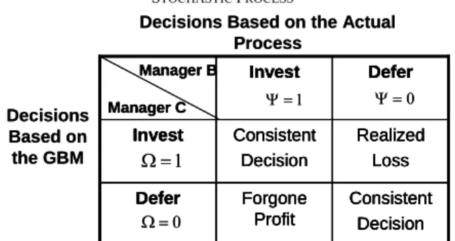
For the purpose of simplifying the problem, when facing an investment opportunity, management is given two alternatives only: to invest or to defer the project. Let Ψ and Ω denote binary variables which represent investment decisions made by Manager B and C, respectively. Therefore, Ψ represents the optimal decision, given the correct specification of stochastic process, and Ω is the mistaken decision, given the misspecification of stochastic process. Suppose both Ω and
Ψ can either take 1 (invest) or 0 (defer) in the binary setting. Since Ω and Ψ are independent decisions for the same investment opportunity under consideration, there are four possible outcomes, two of which describe the situations in which have consistent investment decisions and the other two state the situations where mistaken decisions are in place. Table 1 outlines these four possible outcomes due to the misspecification of stochastic process.
TABLE I FOUR POSSIBLE OUTCOMES DUE TO MISSPECIFICATION OF STOCHASTIC PROCESS 0 = Ω 1 = Ω 1 Ψ = Decisions Based on the GBM
Decisions Based on the Actual Process 0 Ψ = Consistent Decision Forgone Profit Defer Realized Loss Consistent Decision Invest Defer Invest Manager B Manager C 0 = Ω 1 = Ω 1 Ψ = Decisions Based on the GBM
Decisions Based on the Actual Process 0 Ψ = Consistent Decision Forgone Profit Defer Realized Loss Consistent Decision Invest Defer Invest Manager B Manager C Consistent Decision Forgone Profit Defer Realized Loss Consistent Decision Invest Defer Invest Consistent Decision Forgone Profit Defer Realized Loss Consistent Decision Invest Defer Invest Manager B Manager C
According to Table 1 it is possible that Manager C may still make investment decisions which are “consistent” with the optimal decisions made by Manager B, even though an underlying process is not correctly specified. On the other hand, it is also possible that Manager C may make mistaken decisions in the situations that he decides to invest as opposed to the optimal decisions to defer the project, or that he decides to defer the project as opposed to the optimal decisions to invest. It is therefore important to distinguish between
(
)
P Ω = Ψ and P
(
Ω ≠ Ψ , both of which are defined as the)
probability of making consistent decisions and the probability of making mistaken decisions, respectively. In the situations where the misspecification of stochastic process occurs, i.e., Ω ≠ Ψ , there are two types of investment losses, which are regarded as realized losses and forgone profits. Realized losses are referred to as negative payoffs due to the actions of launching a project as it should be deferred optimally, i.e.
1 and 0
Ω = Ψ = . On the other hand, forgone profits are defined as relinquished positive profits due to the actions of deferring a project as it should be taken optimally, i.e.,
0 and 1
Ω = Ψ = . Obviously, both realized losses and forgone profits are investment losses which accrue to Manager C due to the misspecification of the stochastic process assumption.
III. RESEARCHMETHODOLOGY
A. Simulation Procedure
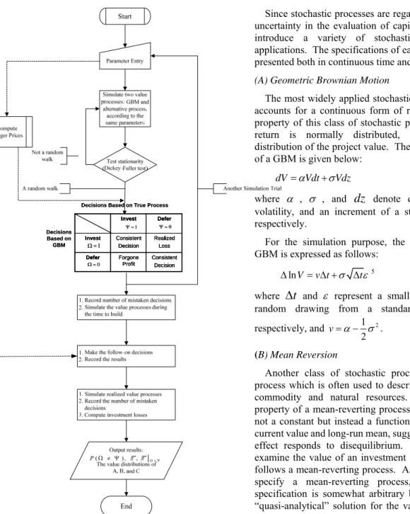
Given the basic investment problem described in the preceding section, a numerical procedure based on Monte Carlo simulation is developed to investigate the trigger price effect and the misspecification effect of stochastic process on the distributions of corporate values. As the first step of simulation, two different stochastic processes, a GBM and an alternative process, are simulated, given the same parameter values. The former is what Manager C believes the underlying process is, while the latter is the actual process which is correctly identified by Manager B. The specifications of stochastic processes of interest are discussed in the next section. To make both processes look like a non-stationary random walk over the licensing period, the Augmented Dickey-Fuller (ADF) p test is conducted to test the null hypothesis that the value process is characterized by a random walk with a possible drift at the level of significance 5%.3 If any of the value process is rejected in the ADF test, the simulation procedure goes back to the beginning and re-simulates a new process according to the same parameter values until the null hypothesis is accepted. Note that the ADF test is conducted only within the licensing period of τ such that both processes may locally resemble a random walk but globally are two different stochastic processes.
The next step is to compute optimal investment triggers based on an alternative process and a GBM, VB∗ and VC∗,
serving as investment decision-making tools. Real options literature suggests that irreversibility and uncertainty complicate investment in that the closed-form solutions of trigger prices are mostly unavailable except those under the assumption of a GBM and a specific form of a mixed diffusion-jump process. If the solution of investment trigger for an alternative process is not available, the general investment framework based on Monte Carlo simulation in [20] is applied to iteratively derive optimal investment trigger. Once both VB∗ and VC∗ are derived, the terminal payoffs of
both simulated stochastic processes over the waiting period are used to determine the optimal decision and the actual decision. In the meanwhile, the net terminal payoffs under an actual process, denoted by
f
, are also computed as a percentage of investment cost, given three types of investment behavior. The net terminal payoffs of Manager A, B, and C, are measured by the following equations, respectively:T A V I f I − = (1)
3 Generally, there are two most commonly used tests for stationarity: the
(Augmented) Dickey-Fuller test and the Phillips-Parron test. The former is essentially a unit root test, where the null hypothesis is a unit root and the alternative is a stationary AR(p) process (the Augmented Dickey-Fuller test is used to test higher order AP process) while the latter is an extension of the Dickey-Fuller test allowing for non-white-noise errors. The DF test is chosen for the reason of ease of computer programming. Refer to [7] for the procedure of hypothesis testing on a random walk.
(
)
, = 0 or 1 T B V I f I Ψ − = ∀Ψ (2)(
)
, = 0 or 1 T C V I f I Ω − = ∀Ω (3)where V is the realized project value, according to the actual T
stochastic process.
It is obvious that when Ω = , 1 Ψ = , and 0 VT< , Manager I
C has a realized investment loss. On the other hand, when 0
Ω = , Ψ = , and 1 VT > , Manager C has a forgone profit. I
By integrating the decision variables, the loss function of Manager C is given as follows:4
(
, ,) (
)(
T)
T V I V I π Ω Ψ = Ω − Ψ − (4) whereπ
denotes the loss ratio of Manager C for a simulation trial.It is important to point out that when there are no delays in collecting project payoffs, V is equal to VT τ. The variables
Ω , Ψ , and π are recorded in each trial. The preceding procedure is to be repeated until the pre-specified simulation trials are completed. In Monte Carlo simulation, the results due to the misspecification of stochastic process are summarized with three performance measures. Let m denote the number of total simulation trials and l be the number of total mistaken decisions within m trials. Thus, if the underlying assumption of stochastic process is misspecified, the probability of making mistaken decisions can be calculated by
(
)
lP
m
Ω ≠ Ψ = (5) There are two types of loss ratios when the misspecification of stochastic process occurs, the unconditional expected loss ratio and the conditional expected loss ratio. The unconditional expected loss ratio is defined as the average loss ratio out of total simulation trials, expressed as follows:
1 l i i m π π =
∑
= (6)The conditional expected loss ratio is referred to as the average loss ratio out of the mistaken decisions, describing the expected value loss of each mistaken decision given that the mistaken decision is made. Therefore, the unconditional expected loss ratio is ex ante and the conditional expected loss ratio is ex post. The conditional expected loss ratio is mathematically expressed as follows:
1 l i i l π π = Ω≠Ψ =
∑
(7)4 Refer to [13] for a similar form of loss function.
( ) , , P Ω ≠ Ψ π π Ω ≠ Ψ Consistent Decision Forgone Profit Defer Realized Loss Consistent Decision Invest Defer Invest 0 = Ω 1 = Ω 1 Ψ = Decisions Based on GBM
Decisions Based on True Process
0 Ψ = Consistent Decision Forgone Profit Defer Realized Loss Consistent Decision Invest Defer Invest Consistent Decision Forgone Profit Defer Realized Loss Consistent Decision Invest Defer Invest 0 = Ω 1 = Ω 1 Ψ = Decisions Based on GBM
Decisions Based on True Process
0 Ψ =
Fig. 1 The Simulation Procedure
It is obvious that the conditional expected loss ratio can be alternatively derived from the unconditional expected loss ratio in Equation (6) divided by the probability of making the mistaken decisions in Equation (5), expressed as follows:
(
)
P π
π Ω≠Ψ =
Ω ≠ Ψ (8) The final output of simulation is the NPV distributions generated from realized project payoffs due to three different types of investment behavior. Figure 1 illustrates the thorough simulation procedure.
B. Stochastic Processes
Since stochastic processes are regarded as major sources of uncertainty in the evaluation of capital investments, here we introduce a variety of stochastic processes for later applications. The specifications of each stochastic process are presented both in continuous time and in discrete time.
(A) Geometric Brownian Motion
The most widely applied stochastic process is GBM which accounts for a continuous form of random walk. The main property of this class of stochastic process is that the rate of return is normally distributed, implying a lognormal distribution of the project value. The continuous-time version of a GBM is given below:
dV =αVdt+σVdz (9)
where α , σ , and
dz
denote drift rate, instantaneous volatility, and an increment of a standard Wiener process, respectively.For the simulation purpose, the discrete-time version of GBM is expressed as follows:
lnV v t σ tε
Δ = Δ + Δ 5 (10) where
Δ
t
and ε represent a small interval of time and a random drawing from a standard normal distribution, respectively, and 1 22
v= −α σ .
(B) Mean Reversion
Another class of stochastic process is a mean-reverting process which is often used to describe the price behavior of commodity and natural resources. The most prominent property of a mean-reverting process is that its growth rate is not a constant but instead a function of a difference between current value and long-run mean, suggesting that growth rate in effect responds to disequilibrium. Dixit and Pindyck [3] examine the value of an investment opportunity whose value follows a mean-reverting process. As there are many ways to specify a mean-reverting process, Dixit and Pindyck’s specification is somewhat arbitrary but convenient to find a “quasi-analytical” solution for the value of the project. The formation of this specific mean-reverting process is given below:
(
)
dV =η V−V Vdt+σVdz (11)
where η denotes a speed of mean reversion and V is a long-run mean.
Equation (11) can be discretized into the following equation:
(
)
1 2 ln 2 V ⎡η V V σ ⎤ t σ tε Δ =⎢ − − ⎥Δ + Δ ⎣ ⎦ (12)5 Since GBM is log-normally distributed, a more explicit form of Equation
(10) is given below:
(v t tt)
t t t
V+Δ = ⎣V e⎡ Δ +σ Δε ⎤⎦
effect on investment in a different way. REFERENCES
[1]. Bar-Ilan, Avner and Strange, William C. “Investment Lags.” American
Economic Review 86 (1996), 610-622.
[2]. Corman, Linda. “To Wait or Not to Wait.” CFO Magazine 13, 5 (1997), 91-94.
[3]. Dixit, Avinash K. and Pindyck, Robert S. Investment under Uncertainty (1994). Princeton University Press, New Jersey, USA.
[4]. Faulkner, Terrence W. “Applying ‘Option Thinking’ to R&D Valuation.” Research Technology Management 39, 3 (1996), 50-56. [5]. Geske, Robert. “The Valuation of Corporate Liabilities as Compound
Options,” Journal of Financial and Quantitative Analysis 12 (1977), 541-552.
[6]. Geske, Robert. “The Valuation of Compound Options.” Journal of
Financial Economics 7 (1979), 63-81.
[7]. Hamilton, James D. Time Series Analysis. Princeton University Press (1994). New Jersey, USA.
[8]. Jensen, Kjeld and Warren, Paul. “The Use of Options Theory to Value Research in the Service Sector.” R&D Management 31, 2 (2001), 173-180.
[9]. Lint, Onno and Pennings, Enrico. “An Option Approach to the New Product Development Process: a Case Study at Phillips Electronics.”
R&D Management 31, 2 (2001), 163-172.
[10]. Majd, Saman and Pindyck, Robert S. “Time to Build, Option Value, and Investment Decisions.” Journal of Financial Economics 18, 1 (1987), 7-27.
[11]. McDonald, Robert and Siegel, Daniel. “The Value of Waiting to Invest.”
Quarterly Journal of Economics 101 (1986), 707-728.
[12]. Merton, Robert C., “Option Pricing When Underlying Stock Returns are Discontinuous.” Journal of Financial Economics 3 (1976), 125-144. [13]. Morgan, M. Granger and Henrion, Max. Uncertainty. Cambridge
University Press (1990). Cambridge, UK.
[14]. Nichols, Nancy A. “Scientific Management at Merck: an Interview with CFO Judy Lewent.” Harvard Business Review 72 (1994), 88-99. [15]. Peeters, Marga. “Investment Gestation Lags: the Difference between
Time-to-Build and Delivery Lags.” Applied Economics 28 (1996), 203-208.
[16]. Pennings, Enrico and Lint, Ono. “The Option Value of Advanced R&D.”
European Journal of Operational Research 103, 1 (1997), 83-94.
[17]. Sender, Gary L. “Option Analysis at Merck.” Harvard Business Review 72 (1994), 92.
[18]. Trigeorgis, Lenos. “Valuing the Impact of the Uncertain Competitive Arrivals on Deferrable Real Investment Opportunities.” Working Paper, Boston University (1990).
[19]. Turvey, Calum G. “Mycogen as a Case Study in Real Options,” Review
of Agricultural Economics 23, 1 (2001), 243-264.
[20]. Wang, Yungchih G. “Topics in Investment Appraisal and Real Options” PhD Thesis, Imperial College, University of London (2004).
Dr. George Yungchih Wang received his PhD in Finance and Economics from
Imperial College, University of London, UK, and his MBA from University of Connecticut, USA. He is currently an assistant professor at National Kaohsiung University of Applied Sciences, Taiwan, and is also a visiting professor at University of Wisconsin, La Crosse, USA. His major research area is in corporate finance, investment appraisal, and corporate governance.
.