國
立
交
通
大
學
電機學院 電子與光電學程
碩
士
論
文
適用於靜態背景視訊並以型態學處理物件邊緣之
即時視訊切割
Real-time Segmentation of Video with Stationary Background Based on
Morphological Edge Processing
研 究 生:黃奕善
指導教授:林大衛 教授
適用於靜態背景視訊並以型態學處理物件邊緣之
即時視訊切割
Real-time Segmentation of Video with Stationary Background Based on
Morphological Edge Processing
研 究 生:黃奕善 Student: I-Shan Huang
指導教授:林大衛 Advisor: Dr. David W. Lin
國 立 交 通 大 學
電機學院 電子與光電學程
碩 士 論 文
A Thesis
Submitted to College of Electrical and Computer Engineering National Chiao Tung University
in Partial Fulfillment of the Requirements for the Degree of
Master of Science in
Electronics and Electro-Optical Engineering June 2007
Hsinchu, Taiwan, Republic of China
適用於靜態背景視訊並以型態學處理物件邊緣
之即時視訊切割
研究生: 黃奕善
指導教授: 林大衛 教授
國立交通大學 電機學院 電子與光電學程碩士班
摘要
在本論文中,我們設計並實現一個在個人電腦上的視訊影像切割系統。此 系統可以應用於靜態背景的視訊電話及視訊會議。 此系統的基本概念是利用物件的邊緣銳化來精準得到移動的物件。首先,我 們使用一個兩級的雜訊估計方法來估計攝影機的雜訊,並且把此結果拿來當做往 後參數調整的參考。為了取得一個較佳的物件遮罩,我們觀察六張連續畫面的變 化情形來取得一個初步的前景以及利用連續兩張畫面的差異選擇一適合的臨界 值將移動的物件萃取出來。接著,我們利用 Canny edge detector 偵測出整張畫面 的邊界資訊,利用影像變動偵測所得之遮罩及前一張畫面所求得之物件遮罩可以 將屬於背景的邊界移除,然後使用收縮的技巧來取得一個粗略的物件遮罩,並利 用此資訊來取得移動物件最外圍之邊界資訊。為了得到更精確的物件遮罩,我們 使用 Dijkstra 所提之最短路徑搜尋演算法,將物件的邊緣連接並利用此封閉的物 件輪廓將移動的物件給萃取出來。最後的模擬結果顯示我們所提的方法,切割出 來的物體邊界是相當精確的,且在經過我們的加速之後,整個系統能快速且精準 的切割出移動的物件。 在 1.733-GHz CPU 及 1024-MB RAM 的個人電腦上且攝影機不移動時,目 前的執行速度是每秒約四張 CIF Frame 及每秒約二十張 QCIF Frame,在格式影 片的應用上,我們有提出一簡化的方法,則每秒約十二張。Real-Time Segmentation of Video With
Stationary Background Based on Morphological
Edge Processing
Student: I-Shan Huang
Advisor: Dr. David W. Lin
Degree Program of Electrical and Computer Engineering
National Chiao Tung University
Abstract
In the thesis, we consider the design and implementation of video segmentation on a personal computer. The system can be applied on video conference and videophone with stationary background.
The basic idea of the system is a graph-based edge linking technique. At first, we adopt a two staged method for camera noise estimation and those thresholds are adjusted based on the estimated camera noise. To get the change detection mask, we consider six consecutive frames as time of observation to estimate the background and select a suitable threshold to estimate the foreground by two consecutive frames. Next, we use Canny edge detector to get the edge information of entire frame. We use the change detection mask and the moving object mask of previous frame to remove the edges of background. Then, we shrink the object mask to edge map. To refine the object mask, we use Dijkstra’s shortest path search algorithm to link the boundary of moving object and extract the object by the closed contour. Simulation results show
that our method can give correct segmentation results. After optimization, the proposed segmentation system can get the moving object accurately and quickly.
With a Intel Pentium M 1.733 GHz CPU and 1024-MB RAM, the system can achieve 20 QCIF frames per second and 4 CIF frames per second. We also propose a simple method and it can achieve 12 CIF frames per second.
誌
謝
本篇論文的產生,最感謝的是我的指導教授-林大衛老師。身為一位在職 研究生要兼顧研究學習及工作本來是件不容易的事,但老師給予我多方面的協助 與鼓勵,讓我在研究學習中能夠順利進行,使我在研究學習及工作中得以兼顧而 能完成本篇論文。老師除給了我完善的專業知識訓練外,在論文實作部份,老師 更培養了我認真踏實的的研究態度,讓我獲益良多。 實驗室完善的資源,讓我可以順利的克服許多實作上所遇的的困難。感謝 學弟介遠、政達,在你們的討論與幫助下,讓我在工作中亦保有快樂的研究生生 涯。 最後,要特別感謝我的爸媽。他們給了我精神上的支持與鼓勵,陪伴我度 過所有的艱難。在此,我要將我的論文獻給所有關心與幫助我的人。 黃奕善 民國九十六年七月於新竹
Contents
1 Introduction 1
2 Overview of Video Segmentation 3
2.1 Meaning of Segmentation . . . 3
2.2 Basic Procedure of Segmentation . . . 3
2.3 Change Detection-Based Technique . . . 5
2.4 Background Subtraction-Based Technique . . . 6
2.5 Graph-Based Edge Linking Technique . . . 10
2.6 Summary . . . 12
3 The Proposed Segmentation Method 14 3.1 System Overview . . . 14
3.2 Two-Stage Noise Estimation . . . 14
3.2.1 Influence of Noise . . . 14
3.2.2 Motivation for Noise Estimation . . . 16
3.2.3 Camera Noise Model . . . 16
3.2.4 Procedure for Two-Stage Noise Estimation . . . 16
3.3 Temporary Moving Object Mask . . . 22
3.3.1 Foreground Estimation . . . 22
3.3.2 Mathematical Morphological Operator . . . 23
3.3.3 Background Estimation . . . 23
3.3.4 Obtaining Initial Object Mask . . . 25
3.4 Edge Linking for Moving Object . . . 29
3.4.1 Find the Candidate of Edge Map . . . 32
3.4.2 Overview of Shortest Path Algorithm . . . 32
3.4.3 Edge-Link Method . . . 35
3.5 Post-Processing . . . 35
3.6 Temporal Filtering . . . 37
3.7 Conclusion . . . 39
4 Optimized Implementation on Personal Computer 42 4.1 Optimization of Algorithm . . . 42
4.2 Overview of Intel’s MMX Technology . . . 44
4.2.1 The MMX Architecture [16], [17], [18] . . . 44
4.2.2 The MMX Instruction Set [18] . . . 47
4.3 Code Acceleration . . . 52
4.3.1 Labeling Function Optimization . . . 52
4.3.2 Edgelink Function Optimization . . . 54
4.3.3 Post processing Function Optimization . . . 56
4.3.4 Erosion and Dilation Function Optimization . . . 58
4.4 Conclusion . . . 60
5 Simulation Results 63 5.1 Segmented Object Masks . . . 63
5.1.1 Segmentation Results . . . 63
5.1.2 Performance Evaluation . . . 64
5.2 Run-time Analysis . . . 64
5.3 Complexity Analysis . . . 69
6 Integration of System on Personal Computer 76 6.1 Video Capturing . . . 77
6.1.1 Video for Windows . . . 77
6.1.3 Implementation of Capture . . . 78
6.2 Result Display . . . 79
6.3 Graphed User Interface . . . 79
6.4 Conclusion . . . 80
List of Tables
4.1 Profile and Run Time Comparison of Claire Sequence (CIF) . . . 43
4.2 Run Time of Optimization of Labeling Function per Frame . . . 44
4.3 MMX Instruction Set Summary (from [19]) . . . 49
4.4 MMX Instruction Set Summary (from [19]) . . . 50
4.5 Run Time of Optimization of Labeling Function per Frame . . . 54
4.6 Run Time of Optimization of Edgelink Function per Frame . . . 56
4.7 Run Time of Optimization of Post process Function per Frame . . . 58
4.8 Run Time of Optimization of Erosion and Dilation Function per Frame . . 58
4.9 Profile and Run Time Comparison of Claire Sequence (CIF) in Debug Mode 61 4.10 Run Time Comparison of Claire Sequence (CIF) in Debug Mode and Re-lease Mode . . . 62
5.1 Profile and Run Time Comparison of Akiyo Sequence (CIF) in Debug Mode 71 5.2 Profile and Run Time Comparison of LabI Sequence (CIF) in Debug Mode 72 5.3 Run Time and Frame Rate of Different Sequences with CIF or QCIF For-mats in Release Mode . . . 73
5.4 Run Time and Frame Rate of Different Sequences use Simple Segmenta-tion Method in Release Mode . . . 73
5.5 Comparison of Run-time between Different Algorithms . . . 74 5.6 Complexity of Major Algorithms in One CIF Frame of Claire Sequence . 75
List of Figures
2.1 A basic segmentation system (from [8]). . . 4
2.2 Background subtraction-based segmentation system (from [4]). . . 8
2.3 Initial object mask generation (from [4]). . . 9
2.4 Graph-based edge linking segmentation system (from [5]). . . 11
2.5 Correction of a boundary segment. (a) Enlarged portion of the wrong boundary. (b) Corresponding binary model points. (c) Weights assigned for Dijkstra’s algorithm. (From [5]). . . 13
3.1 The block diagram of proposed method. . . 15
3.2 A thresholded frame difference map of the Mother-and-Daughter sequence (from [8]). . . 17
3.3 A thresholded frame difference map of the Akiyo sequence (from [8]). . . 17
3.4 A frame difference map of Mother-and-Daughter sequence (from [8]). . . 19
3.5 Four masks of directional sums (from [8]). . . 19
3.6 Mother-and-Daughter sequence (from [8]). . . 19
3.7 Claire sequence (from [8]). . . 20
3.8 Noise estimation of Mother-and-Daughter sequence (from [8]). . . 20
3.9 Noise estimation of Claire sequence (from [8]). . . 21
3.10 Noise estimation of Mother-and-Daughter sequence for the two-stage method (from [8]). . . 21
3.11 Noise estimation of Claire sequence for the two-stage method (from [8]). 22 3.12 Threshold frame difference map of frame 27 in Claire sequence. . . 24
3.13 Threshold frame difference map of frame 27 in Claire sequence after clos-ing operation. . . 24 3.14 The original frame 60 in Claire sequence. . . 26 3.15 Threshold frame difference map after foreground estimation of frame 60
in claire sequence. . . 26 3.16 Threshold frame difference map after background estimation of frame 60
in Claire sequence. . . 27 3.17 The OR map of Fig 3.15 and Fig 3.16. . . 27 3.18 Threshold frame difference map after remove small region of frame 60 in
Claire sequence. . . 28 3.19 Threshold frame difference map after fill-in of frame 60 in Claire
se-quence . . . 28 3.20 Edge map of frame 60 in Claire sequence. . . 30 3.21 Edge map after opening operator of frame 60 in Claire sequence. . . 30 3.22 Edge map after removing background edges of frame 60 in Claire sequence. 30 3.23 Final object edge map of frame 60 in Claire sequence. . . 31 3.24 Final object mask of frame 60 in Claire sequence. . . 31 3.25 The edge map of frame 49 after Canny operation in Mother-and-Daughter
sequence. . . 33 3.26 The edge map of frame 49 after removing background edges in
Mother-and-Daughter sequence. . . 33 3.27 The outmost edge map of frame 49 in Mother-and-Daughter sequence. . . 34 3.28 The weighted edge map of frame 49 in Mother-and-Daughter sequence. . 34 3.29 Flowchart of edge-link method. . . 36 3.30 The edge map of frame 49 after edge-link in Mother-and-Daughter
se-quence. . . 36 3.31 The object mask of frame 49 after padded with edge pixels in
Mother-and-Daughter sequence. . . 38 3.32 The original frame 49 in Mother-and-Daughter sequence. . . 38 3.33 The moving object of frame 49 in Mother-and-Daughter sequence. . . 38
3.34 Flowchart of temporal filter. . . 39
3.35 Segmentation of the Claire sequence. (a) The original frame 29. (b) The original frame 30. (c) The original frame 31. (d) Frame 29 without tem-poral filter. (e) Frame 30 without temtem-poral filter. (g) Frame 31 without temporal filter. (g) Frame 29 with temporal filter. (h) Frame 30 with tem-poral filter. (i) Frame 31 with temtem-poral filter. . . 40
4.1 The object mask after applying down-sample. . . 45
4.2 The object mask after applying labeling and up-sample. . . 45
4.3 MMX packed data types (from [16]). . . 47
4.4 MMX register set (from [19]). . . 48
4.5 PACKSSDW instruction operation using 64-bit operands (from [18]). . . 51
4.6 Section of code that we would like to optimize with MMX. . . 53
4.7 Code in Fig. 4.6 after optimization using MMX instructions. . . 53
4.8 The section of original code with malloc function. . . 55
4.9 The section of revised code with calloc function. . . 55
4.10 The section of original code without break instruction. . . 55
4.11 The section of revised code with break instruction. . . 56
4.12 Section of code that we would like to optimize with MMX. . . 57
4.13 Code in Fig. 4.12 after optimization using MMX instructions. . . 57
4.14 The section of original code without continue instruction. . . 59
4.15 The section of original code with continue instruction. . . 59
5.1 Segmentation of the Mother-and-Daughter sequence. (a) Frame 48. (b) Frame 156. (c) Frame 234. (d) Segmented object in frame 48. (e) Seg-mented object in frame 156. (f) SegSeg-mented object in frame 234. . . 65
5.2 Segmentation of the Claire sequence. (a) Frame 16. (b) Frame 63. (c) Frame 104. (d) Segmented object in Frame 16. (e) Segmented object in Frame 63. (f) Segmented object in Frame 104. . . 66
5.3 Segmentation of the Akiyo sequence. (a) Frame 24. (b) Frame 60. (c) Frame 141. (d) Segmented object in Frame 24. (e) Segmented object in
Frame 60. (f) Segmented object in Frame 141. . . 67
5.4 Segmentation of the LabI sequence. (a) Frame 18. (b) Frame 19. (c) Frame 20. (d) Segmented object in frame 18. (e) Segmented object in frame 19. (f) Segmented object in frame 20. . . 68
5.5 Fractional agreement between the segmented foreground object of the Akiyo sequence and the reference mask. . . 68
5.6 Flowchart of simple segmentation method. . . 70
6.1 System block diagram (from [8]). . . 76
6.2 Circumstance of implementation (from [8]). . . 77
6.3 AVI header (from [8]). . . 78
6.4 Related code for creating a capture window. . . 78
6.5 Related code for parameter modification. . . 79
6.6 Related code for capture operation. . . 79
6.7 Related code for displaying. . . 80
Chapter 1
Introduction
We consider the design and implementation of video segmentation system on a personal computer. The intended application is PC-based videoconference and videophone system. We assume the camera is fixed.
Video segmentation is one of the fundamental technologies for content-based real-time MPEG-4 camera system. For real-real-time requirement, the segmentation algorithm should be fast and accurate. The main objective in segmentation is to partition the data into meaningful and independent regions. According to the type of data, we can classify the processes into image segmentation and video segmentation. Here, we focus on the video segmentation. The general schemes for video segmentation can be seen as the following steps: pre-processing, feature extracting, decision, and post-processing. In this thesis, a method based on change detection and graph-based edge linking is proposed.
The basic idea of the system is a graph-based edge linking technique. The moving objects of current frame can be roughly obtained by the change detection technique. It requires statistical modeling of the background noise. To begin, we estimate the vari-ance of the background noise by finding the difference of consecutive frames. Then we obtain a compact image region by a fill-in procedure employing the edge map from em-ploying the Canny method. However, typical edge detection algorithms, including the Canny method [1], do not yield closed region contours or fully connected curves at object boundaries. To help object segmentation, we employ a shortest-path algorithm to find and
After linking edge, we could obtain a closed object boundary. The postprocessing is to eliminate the redundant region and smooth the object boundary. To smooth the boundary, morphological operations are applied. At last, the object alpha map is generated after this process.
The technologies described as above deal with the video in spatial domain in addition to change detection. In temporal domain, we use the temporal filter. The simplest way to judge whether the value of a pixel is background is to check the alpha map at this location. Our idea is to record the weight of variability of consecutive alpha frames. If the weight is greater than the threshold, the pixel is considered that stationary.
In many steps of our algorithm, we need a threshold to make decisions. In many situations, the threshold is adjusted to counteract the influence of noise and therefore we estimate the camera noise at first and the adjustment of threshold is based on camera noise.
We propose an automatic segmentation system which include change detection, back-ground registration, and graph-based edge linking techniques. At first, we modify and integrate these techniques to get the most accurate object mask. Second, we improve the system to achieve the real-time requirement. Finally, we integrate our segmentation system on personal computer to test natural video sequence.
This thesis is organized as follows. Chapter 2 is an overview of popular video seg-mentation techniques. Chapter 3 gives a detailed description of proposed segseg-mentation method. Chapter 4 discuss the optimization of proposed video segmentation method. Chapter 5 shows the simulation result. Chapter 6 shows the integration of the proposed segmentation method on the personal computer. Chapter 7 contains the conclusion and future work.
Chapter 2
Overview of Video Segmentation
2.1 Meaning of Segmentation
The main objective in segmentation is to partition the data into meaningful and indepen-dent regions. According to the type of data, we can classify the segmentation processes into image segmentation and video segmentation. In the case of image segmentation, the problem is two-dimensional in nature, while in case of video segmentation, in addition to the two-dimensional information we can also handle the problem with the aid of motion information.
The algorithm of segmentation depends to a large extent on the application and the data that are used. In one application, partition into ten regions may be ideal but for an other application partition into two regions may be desired. In the ideal case, we may develop a best algorithm for each application but it likely come with very high complexity. In practice, we often develop an algorithm best suited to specific applications, not to general situations.
2.2 Basic Procedure of Segmentation
In [8], the author mention that a general scheme for segmentation can be seen as composed of the following steps: pre-processing, feature extraction, decision, and post-processing,
Figure 2.1: A basic segmentation system (from [8]). 1. Pre-processing:
The original data may include a high amount of information but most of it is irrel-evant to our application and sometimes influences our decision. In the stage, we remove the irrelevant information and keep the desired data.
2. Feature extraction:
Depending on various segmentation algorithms, we need some specific features to achieve our goals. In this stage, we extract the desired features from original data. 3. Decision:
The values of extracted features are usually more than two values and therefore we need to find a threshold to classify those data. In the stage, we can use many strategies to make a desired threshold set to find out the regions which meet our goal.
4. Post-processing:
Although we can use many decision strategies to make a best threshold set, we may still make wrong decisions in some special regions. In the stage, we will try to correct those improper regions.
2.3 Change Detection-Based Technique
It is possible to extract the independently moving objects from background by calculating frame difference between consecutive frames. This technique is usually named change detection. The main advantage of change detection is that it has relatively low computa-tional complexity and can extract the moving objects roughly. Many video segmentation algorithms employ this technique for simplicity.
Change detection algorithms usually start with the gray value difference map between the two frames considered. The local sum (or mean) of absolute difference is computed inside a small measurement window which slides over the difference map. At each lo-cation, this local sum of absolute differences is compared against a threshold. Whenever this threshold is exceeded, the center pixel of the current window location is marked as changed. The key issue of this technique is how to decide the threshold.
The algorithm in [3] provides some statistical methods to decide the threshold. It starts by computing the gray level difference image D = {dk}, with dk = y1(k) −
y2(k), between two considered pictures Y1 = {y1(k)} and Y2 = {y2(k)}. The index k
denotes the pixel location on the image grid. Under the hypothesis that no change occurs at location k, the corresponding difference dk obeys a zero mean Gaussian distribution
N(0, σ) with variance σ2, that is,
p(dk|H0) = 1 √ 2πσ2 exp{− d2 k 2σ2}. (2.1)
Since the camera noise is uncorrelated between different frames, the variance σ2 is
equal to twice the variance of the assumed Gaussian camera noise distribution. H0denotes
the null hypothesis, i.e., the hypothesis that there is no change at pixel k. The unknown parameter σ can be estimated offline for the used camera system, or recursively online.
In order to make the detection more reliable, a region may be used to evaluate the difference di instead of only a single pixel. One may thus compute the local sum 42i of
(dk
σ)2 inside a small sliding window wi, with i denoting the center pixel of the window.
The local sum 42
i is proportional to the sample mean of (dσk)2 as computed inside the
N(0, 1) with variance 1. Thus, the sum 42
i obeys a χ2-distribution with as many degrees
of freedom as there are pixels inside the window. With the distribution p(42|H
0) known,
the decision between “changed” and “unchanged” can be arrived at by a significance test. For this purpose, one may usually specify a significance level α and compute a corresponding threshold tα according to
α = P rob(42i > tα|H0). (2.2)
The statistic 42
i is now evaluated at each location i on the image grid, and whenever
it exceeds tα, the corresponding pixel is marked as changed, otherwise as unchanged.
The method given above exhibits some shortcomings. First, there are inevitably deci-sion errors. Typically, these errors appear as small isolated spots inside correctly labeled regions. Another drawback is that in some critical image areas the boundaries between differently classified regions tend to be somewhat irregular. To avoid these shortcomings, the MAP (maximum a posteriori) criterion can be used to get a better change mask. That is to say, one may try to find the change mask Q = qk which maximizes the a posteriori
density p(Q|D), where D is the given difference image. The label qk at location k can
take either the value u for “unchanged” or c for “changed”. After a series of deduction, we can get the final decision rule as
d2k u > < c 2 σ2cσ2 σ2 c− σ2 (lnσc σ + (vB(c) − vB(u))B + (vC(c) − vC(u))C). (2.3)
where B is a positive cost term of each horizontally or vertically oriented border pixel pair and C is that of diagonally pair, and vB(qk) and vC(qk) denote the number of
inho-mogeneous cliques to which pixel k belongs when its label is qk.
2.4 Background Subtraction-Based Technique
The idea of background subtraction is to subtract the current image from the still back-ground, which is acquired before the objects move in. After subtraction, only non-stationary or new object are left. The most straightforward way to separate background is to apply a simple difference and threshold method.
An example of background subtraction-based technique is proposed in [4]. This seg-mentation system consists of five major steps as shown in Figure 2.2.
1. Frame difference:
The frame difference mask is generated simply by thresholding the frame differ-ence. This data is sent to the background registration step where the reliable back-ground is constructed from the accumulated information of several frame difference masks. Since the accumulated frame difference mask are used in the final decision for a reliable background, no filtering or boundary relaxation is applied on the frame difference.
The changed detection technique as show in last section is used to obtain the thresh-old value.
2. Background registration:
The goal of background registration is to construct a reliable background informa-tion from the video sequence. In this applicainforma-tion, it needs a reliable background information for change detection.
The history of frame difference mask is considered in constructing and updating the background buffer. A stationary map is maintained for this purpose. If a pixel is marked as changing in the frame difference mask, the corresponding value in the stationary map is cleared to zero; otherwise, if the pixel is stationary, the corre-sponding value is incremented by one. The values in the stationary map indicate that the corresponding pixel has not been changing for how many consecutive frames. If a pixel is stationary for the past several frames, then the probability is high that it belongs to the background region. Therefore, if the value in the stationary map exceeds a predefined value, then the pixel value in the current frame is copied to the corresponding pixel in the background buffer.
A background registration mask is also changed in this process. The value in the background registration mask indicates that whether the background information
background buffer, the corresponding value in the background registration mask is changed from nonexisting to existing.
3. Background difference:
This step generates a background difference mask by thresholding the difference between the current frame and the background information stored in the background buffer. This step is very similar to the generation of frame difference mask.
4. Object detection:
The object detection step generates the initial object mask from the frame differ-ence mask and the background differdiffer-ence mask. The background registration mask, frame difference mask, and background difference mask of each pixel are required information. Figure 2.3 lists the criteria for object detection, where BD means the absolute value of difference between the current frame and the background informa-tion stored in the background buffer, F D is the absolute value of frame difference, and the OM field indicates that whether or not the pixel is included in the object mask. T HBD and T HF D are the threshold values for generating the background
difference mask and frame difference mask, respectively. If BD is greater than
T HBD, the pixel would be judged belong to moving object. If the BD is not
ex-ist, it would depend on the F D to judge the pixel change or unchange. And the condition is the same as change detection technique.
5. Post-processing:
After the object detection step, an initial object mask is generated. However, due to the camera noise and irregular object motion, there exist some noise regions in the initial object mask. The approach to eliminate the noise region relies on an observation that the area of noise regions tend to be smaller than the area of the object. Regions with area smaller than a threshold value are removed from the object mask. In this way, the object shape information is preserved while smaller noise regions are removed. After removing noise regions, a close and an open operation with a 3 × 3 structuring element are applied on the object mask.
2.5 Graph-Based Edge Linking Technique
In [5],[6],[7], authors proposed an automatic video segmentation algorithm based on graph-based edge linking technique. The algorithms link up the boundaries of the moving object to extract the moving object. In the following we will show a system proposed in [5] in which the edge linking technique is used. The system incorporates edge tracking has been proposed. A dense optical flow field and a global affine motion model has been computed to derive the motion mask. After the initial binary model for the interest is derived, the object tracker matches the model against subsequent frames in the sequence and updates the model. The basic idea of the algorithm is shown in Figure 2.4.
In the block of Video Object Plane (VOP) Extraction, the shortest path algorithm has been applied in order to correct the incorrect object boundaries resulting from the use of the filling-in procedure. Each wrong boundary segment is corrected separately. After removing one of those, there will be a gap in the otherwise closed contour, as illustrated in Figure 2.5(a).
Naturally, the contour between A and B should coincide with binary model points, which are showed in Figure 2.5(b). Hence, a small weight or distance d0 is assigned
to these model points. The weight is also set to d0 for all pixels along the four frame
boundaries, because in many situations they form part of the VOP contour. All remaining pixels are less likely to belong to the VOP boundary and a weight d1 with d1 > d0 is
corrected boundary segment. Therefore, all pixels that already belong to the VOP contour after removing the wrong boundary segment must be excluded. This is accomplished by setting the corresponding weights to infinity. To summarize, pixels that already belong to the VOP boundary must be excluded from the search by assigning infinity or a suitably large distance to them. The distance is set to d0 both for object model points that are
not yet VOP boundary pixels and for pixels along the four frame boundaries. All other pixels have a weight of d1. Figure 2.5(c) visualizes the weights assigned to the pixels in
example.
This technique has to link the boundaries of moving object and get the closed contour. It can extract the moving objects for accurate locating of moving object boundaries. But this scheme is quite computationally expensive.
2.6 Summary
All techniques described above can obtain a desired object mask. Here, we explain the reason why we employ these techniques. In our application, the camera is fixed. For real time requirement, we employ the change detection-based technique to get the moving objects roughly because it can avoid complex computation. The object masks obtained by change detection-based technique are hard to resist the camera noise and the accuracy of object mask is hard to keep for the entire sequence. So we employ graph-based edge linking technique to get the closed contour of moving object and use it to refine the object masks.
However, since the behavior and characteristics of the moving objects differ signifi-cantly, the quality of segmentation result depends strongly on background noise, object motion, and the contrast between the object and the background. Reliable and consistent object information from the changing part of the scene is not easy to maintain for the entire sequence, we concentrate on the stationary background where the characteristics are well known and more reliable. So we employ the background registration technique in temporal domain to smooth the boundaries of moving object.
Figure 2.5: Correction of a boundary segment. (a) Enlarged portion of the wrong bound-ary. (b) Corresponding binary model points. (c) Weights assigned for Dijkstra’s algo-rithm. (From [5]).
Chapter 3
The Proposed Segmentation Method
3.1 System Overview
Our segmentation system employs a graph-based edge linking scheme. The block dia-gram is shown in Figure 3.1. To start, we estimate the camera noise and the following thresholds are decided according to estimated camera noise. We use the foreground es-timation and background eses-timation to generate the object mask. The edge map can be obtained by Canny operator in current frame. We can remove the edges of background and shrinks object mask to edge map. According to shortest path algorithm, we can get the closed contour of moving object. In the step of postprocessing we refine the object mask and get accurate object mask. The boundaries of moving object can be smoothed by temporal filter.
In this system, most of these modules are used for processing each frame. The details of this system are discussed in the following sections.
3.2 Two-Stage Noise Estimation
3.2.1 Influence of Noise
In this system, the image is captured by camera and then we get the initial image from the output of camera. In the process of capturing, the image may suffer from camera
noise and therefore the stationary background usually has some difference between suc-cessive frames. In general, larger camera noise makes good segmentation more difficult to achieve. For example, when change detection-based technique is applied, the frame difference map of larger noise sequence (Figure 3.2) includes more background pixels than smaller noise sequence (Figure 3.3). It is apparent that the larger noise sequence needs more processing to obtain a better object mask.
3.2.2 Motivation for Noise Estimation
In the following steps of the system, we need many thresholds or parameters to make decisions and those thresholds are usually adjusted to counteract the influence of noise. We can adjust those parameter empirically but it is inconvenient since we have to tune them for different situations and it usually needs some experiences. In order to reduce the complexity of threshold decision, those parameters in the following steps are adjusted based on estimated camera noise.
3.2.3 Camera Noise Model
In the thesis, we assume the difference dkof stationary pixels between successive frames
obeys a zero mean Gaussian distribution N(0, σ) with variance σ2, that is,
p(dk|H0) = 1 √ 2πσ2exp{− d2 k 2σ2}. (3.1)
where H0 denotes the null hypothesis. As in [3], since the camera noise is uncorrelated
between different frames, the variance σ2 is equal to twice the variance of the assumed
Gaussian camera noise distribution.
3.2.4 Procedure for Two-Stage Noise Estimation
In order to estimate the variance σ2, the sample space should include those pixels
belong-ing to stationary background and exclude pixels belongbelong-ing to movbelong-ing objects. Our idea to discriminate the two kind of pixels is based on the observation which can be seen in Fig-ure 3.4. The lighter pixels which represent larger difference are usually lumped together
Figure 3.2: A thresholded frame difference map of the Mother-and-Daughter sequence (from [8]).
or are distributed like a strip when they are introduced by moving objects. On the other hand, the larger frame differences caused by camera noise are usually randomly distrib-uted. Hence, we reject the pixels whose neighbors have larger frame difference from the sample space during noise estimation.
We use the same mask of [11] to find out those pixels that belong to moving objects. For each pixel, we consider the four directional sums in frame difference map as shown in Figure 3.5. If one of the four directional sums is larger than certain threshold, we can assume that the pixel belongs to a moving object.
The following problem is how we choose the threshold. Up to the present, we can only calculate variance σ2
G of frame difference of entire frame, and therefore it is natural that
we initially adjust the threshold based on σ2
G. If one of the four directional sums of a pixel
is larger than ασ2
G, the pixel is classified to pixels influenced by moving objects. After we
remove those pixels influenced by objects, those remaining pixels are used to estimate σ2.
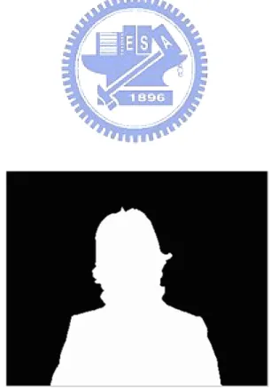
In order to verify the result of our method, we first manually choose the pixels belonging to stationary background to estimate the variance σ2. In Figures 3.6 and 3.7, the white
areas are chosen to estimate σ2 and the estimation result is regarded as exact. As we can
see in Figures 3.8 and 3.9, this method can effectively remove most pixels influenced by moving objects.
It is obvious that the results in Figures 3.8 and 3.9 are still influenced by moving objects, because we adjust the threshold based on variance σ2
G of entire frame which has
high relationship with moving objects. In order to reduce this problem, we use a two-stage noise estimation in this system. In the first stage, we use the ασ2
G (In the experiment, α
is 25) to be the threshold and get the variance σ2
1 of stage one. In the second stage, we
use the βσ2
1 (In the experiment, β is 20)as the threshold and then we can obtain the final
result σ2
2 of stage two. The final result is shown in Figures 3.10 and 3.11. It can be seen
Figure 3.4: A frame difference map of Mother-and-Daughter sequence (from [8]).
Figure 3.7: Claire sequence (from [8]).
Figure 3.9: Noise estimation of Claire sequence (from [8]).
Figure 3.10: Noise estimation of Mother-and-Daughter sequence for the two-stage method (from [8]).
Figure 3.11: Noise estimation of Claire sequence for the two-stage method (from [8]).
3.3 Temporary Moving Object Mask
In this section, we will generate a temporary foreground mask and then the mask is used to get the outmost edge map of moving object. In this stage, we use change detection-based technique to obtain a rough mask. The major advantage of this technique is that the frame difference can be easily and speedily obtained. Then we use the binary morphological operator to remove small regions that arise due to camera noise. After these steps we can get a rough moving object mask in this stage.
3.3.1 Foreground Estimation
A moving object is also called foreground and the stationary parts are called background. At first, we use the 3 × 3 window to calculate the mean of squared frame difference for each pixel. If the result is larger than threshold, the pixel is classifed as in a moving object. On the other hand, a pixel is classified as background when the result is smaller than threshold. The threshold here is adjusted based on the camera noise, that is, γσ2.
shown in Figure 3.12.
3.3.2 Mathematical Morphological Operator
The output of thresholded frame difference map is binary image. The pixels of foreground are marked in white. As shown in Figure 3.12, there are many small regions which are marked in white and they do not belong to foreground. So we use morphology operator to delete them and make the pixels of foreground to lump together.
Mathematical morphology is a well-known set theoretic and shape oriented approach which treats the image as a set and the kernel of operation, dilation, erosion, opening, closing, etc., as another set. Each operation set, namely structuring element, plays an important role in dealing with shape or extracting features from the image. The structuring element is a kind of coefficients set in mathematical morphology. In digital image, there are two popular kinds of structuring elements, 4-connectivity and 8-connectivity.
In our application, we select the 3 × 3 and 8-connectivity structuring elements. The operation of binary erosion means if one of 8-connectivity pixels is marked black, then the central pixel is marked black. The operation of binary dilation means if one of 8-connectivity pixels is marked white, then the central pixel is marked white. The opening and closing operators are composed of erosion and dilation. In [9], closing operator can remove the salt noise and opening operator can remove pepper noise. So we employ closing operator to the thresholded frame difference map and the result is as shown in Figure 3.13.
3.3.3 Background Estimation
To obtain the robust moving object mask, we employ the background estimation in the same time.
The simplest way to judge whether the value of a pixel is background is to check the frame difference at this location. Since moving objects will cause larger frame difference, we can assume that a pixel belongs to background at this location when the frame dif-ference at this location is very small from start to finish. For real-time application, it is
Figure 3.12: Threshold frame difference map of frame 27 in Claire sequence.
Figure 3.13: Threshold frame difference map of frame 27 in Claire sequence after closing operation.
impossible to make a decision after whole data is collected from beginning to end. In the system, we regard the value of pixel as background when its frame difference is small for some consecutive frames.
We consider six consecutive frames fk(i) (1 ≤ k ≤ 6) as the time of observation and
a 3 × 3 window is used to calculate frame difference dm(i) = f6(i) − fm(i) (1 ≤ m ≤ 5)
for each location i in a frame. For every location i, we calculate the mean and variance of dm(i) (1 ≤ m ≤ 5). If the variance is smaller than threshold, it means the changes
between the six frames are small and we can regard the value of pixel at location i of sixth frame as background. The threshold here is also based on camera noise, that is, λσ2. The
range of λ is from 2 to 10.
3.3.4 Obtaining Initial Object Mask
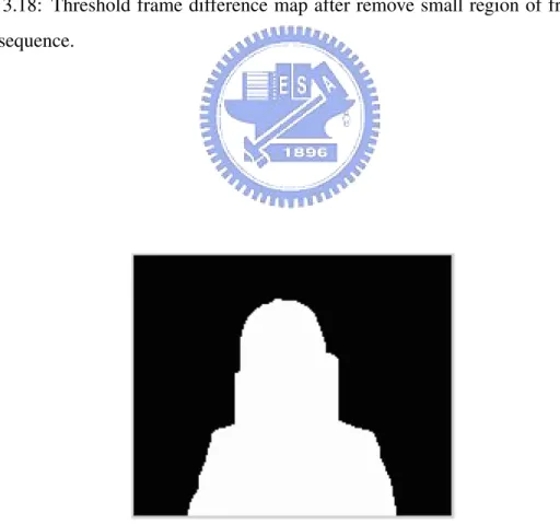
After foreground and background estimation, we can get two thresholded frame difference maps. In this stage, we want to generate the initial moving object mask. At first, we obtain a rough object by ORing the two maps. There might be noise present, which can be suppressed based on the size of connected components in the object mask. In the second step, we label the connected components in the object mask and set a threshold. In the experiment,the threshold is from 10 to 40. If the size of a component exceeds a threshold, we assume it belong to object mask. In the third step, we use the fill-in technique proposed in [5]. The fill-in technique is described as that at first we assign the pixels between the first and last white points of 3.18 to white points for each row. This procedure is then repeated for each column. The step-by-step results are shown in Figures 3.15 to 3.19.
3.3.5 Refining Initial Object Mask
Since the fill-in technique always marks the region between left and right boundaries, there are some pixels belong to background always regarded as objects. So we refine the object mask. It will be very helpful if the mask here is more accurate.
In this stage, we use the edge information to correct the initial mask and the Canny operator proposed in [1] is adopted to get edge information. The operator performs a
gra-Figure 3.14: The original frame 60 in Claire sequence.
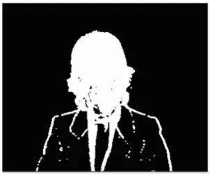
Figure 3.15: Threshold frame difference map after foreground estimation of frame 60 in claire sequence.
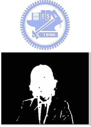
Figure 3.16: Threshold frame difference map after background estimation of frame 60 in Claire sequence.
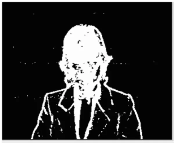
Figure 3.18: Threshold frame difference map after remove small region of frame 60 in Claire sequence.
dient operation on the image which convolutes it with Gaussian filter and then nonmaxi-mum suppression is applied to thin the edge. In the last step, the thresholding operation with hysteresis is used to find and link edges. The thresholding operation including two thresholds: threshold and low-threshold. Pixels whose gradient is larger than high-threshold are regarded as edges and pixels whose gradient is smaller than low-high-threshold are regarded as non-edges. Pixels whose gradient is between high-threshold and low-threshold need to check their neighbors. If one of its neighbors is regarded as edge, these pixels are classified to edge. The edge map after applying Canny operator is shown in Figure 3.20. The related code of Canny operator is obtained from [12].
At first, we employ the opening operator to lump the pixel which is marked in black. The edge map after applying opening operator is shown in Figure 3.21. The way to refine the initial object mask is shrinking the initial mask to fit the edge map. The initial mask, edge map and shrunk mask are shown in Figures 3.22, 3.23 and 3.24, respectively, for Claire sequence. In these figures, we can see that the edge map includes many background edges and those background edges usually interfere with the final result. According to the initial moving object mask, when a position of object mask is marked black, we assume that there is a background edge in the position. The result after removing the background edge can be seen in Figure 3.22. In Figure 3.22, we can find some pixels which belong to background edges. To reduce the influence of those background edges, we use the connected algorithm to delete them. In Figures 3.23 and 3.24, we can see that background edges can be effectively removed and the final object masks are obtained.
3.4 Edge Linking for Moving Object
In our application, we employ the change detection technique to obtain a rough outline of an object. Next, we employ the Canny method [1] for edge detection and remove the background edges. Then, we employ roll operator [8] to shrink the initial object mask to edge map. Edge information is very useful in identifying object boundaries. However, typical edge detection algorithms, including the Canny method, do not necessarily yield closed region contours or fully connected curves at object boundaries. And the change
Figure 3.20: Edge map of frame 60 in Claire sequence.
Figure 3.21: Edge map after opening operator of frame 60 in Claire sequence.
Figure 3.23: Final object edge map of frame 60 in Claire sequence.
detection mask is influenced by camera noise and the intensity of light. So it would lose some edges of moving object. In the section, the outermost edges in the region are identified and linked using a shortest path algorithm.
3.4.1 Find the Candidate of Edge Map
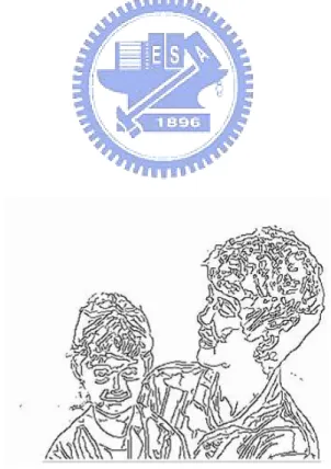
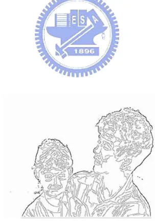
In this stage, we use the Mother-and-Daughter sequence for instance. The edge map after applying Canny operator is shown in Figure 3.25. The edge map after removing background edges is shown in Figure 3.26. Given a set of edges in a region, one common way to obtain a rough outline of the object is by orthogonal scans. Each row that contains edge pixels is considered. The space between the leftmost and the rightmost such pixels is filled in. Likewise, for each column that contains edge pixels, the space between the topmost and the bottommost such pixels is fill in. Then a rough object mask is obtained by ANDing the two pixel map. After the orthogonal scans, we use the 8-connectivity method to get the outmost edges of objects.
The method of connectivity is that if the pixel is marked black and one of its 8-connectivity neighbors is marked white, we consider the pixel belong to the outmost edge pixel of moving object. The result can be seen in Figure 3.27. The others of the edge map is marked gray, as shown in Figure 3.28.
3.4.2 Overview of Shortest Path Algorithm
In [2], the author provides solutions to two graph problems under the following assump-tions. There are n vertices, there exists at least one path between any pair of vertices, and the paths have positive lengths. The first problem is to construct a tree of minimum total length between n vertices, and the second problem is to find the path of minimum total length between two given vertices. In here, we consider the second problem.
To find the shortest path from vertex S to vertex t, the algorithm does the following: 1. Set a variable D[x], x is any vertex. D[x] = 0 when x is equal to S, and D[x] = inf
Figure 3.25: The edge map of frame 49 after Canny operation in Mother-and-Daughter sequence.
Figure 3.26: The edge map of frame 49 after removing background edges in Mother-and-Daughter sequence.
Figure 3.27: The outmost edge map of frame 49 in Mother-and-Daughter sequence.
2. Assume D[x] = min(D[x], D[y] + a(y, x)), a(y, x) is the distance from y to x. Let y = x, if x is not equal to S and x never be assigned to y. For example:
D[S] = 0, D[a] = 5, D[b] = 7, D[c] = 6, the result is y = a.
3. If y = t, the shortest path from S to t is found. Otherwise repeat step 2.
4. Calculate the total number of vertices from S to t and record the number of them.
3.4.3 Edge-Link Method
In this stage, we introduce the edge-link method in our system. After previous step, we can get the outermost edge map and weighted edge map of moving objects. We divide the edge map into two parts. Edge-linking is applied to each part independently. At first, we assign an equivalent length d0 to the pixels which are marked in Figure 3.28, assign an
equivalent length d1to the pixels which are marked white, and assign an equivalent length
inf to the pixels which are marked black. We let d0 = 1, d1 = 10, and inf = 10000 in
the experiments. To control the computational complexity, we may limit the search area to a band around the mask’s boundary. We adopt two search areas, 22 × 22 and 46 × 46, in our system.
Then we find out all vertices and the number of segments. We employ the connected algorithm to calculate the number of segments. We find out the coordinates of start vertex and termination. According to the coordinates, we can divide the direction into first and second quadrants. Then we can transfer the coordinate of vertex to a number. According to the number of vertex, we can employ the shortest path algorithm to link them from bottom to top. The Figure 3.29 shows the flowchart of edge-link algorithm. The result after edge-link is shown in Figure 3.30
3.5 Post-Processing
In this section, we want to refine the object mask and to extract the moving object. After linking the edges of moving object, we get the closed contour. At First, the object mask
Figure 3.29: Flowchart of edge-link method.
the connected algorithm to remove the redundant pixels of moving object and to extract moving object. The algorithm is based on the size of connected components in the object mask. We employ 8-connectivity method to label the connected components which is marked in white and set up a threshold. In the experiment, the threshold is 10000. If the size of a component does not exceed the value, we can assume it does not belong to the object mask. after the step we can get the accurate object mask. The original frame is shown in Figure 3.32. The result after post-processing is shown in Figure 3.33.
3.6 Temporal Filtering
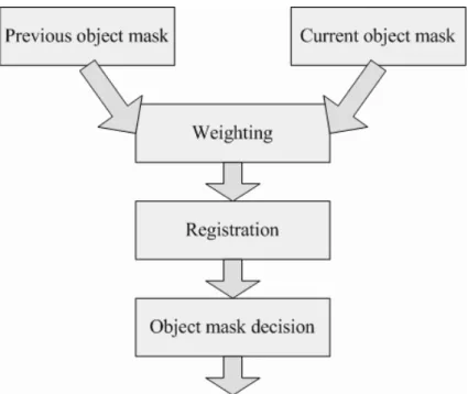
Usually, the object mask does not change violently between the current frame and previ-ous. Based on this, we employ the background registration technique. The flowchart is shown in Figure 3.34.
There is a buffer to store the object mask of previous frame in our system. When we get the first object mask, the temporal filter is started. The step-by-step procedure is as follow:
1. Weighting: Compare the object mask in previous fame and current frame. If the pixel at the same location between the previous and current frames is marked in different colors, we would mark the pixel in gray.
2. Registration: According to the weighting object mask, we prepare a buffer to record the accumulated value. If the pixel is marked black, we assume the pixel belongs to background and add a constant to the buffer. (In the experiment the constant is 10.) If the pixel is marked white, we know it belongs to foreground and we would set the buffer for zero. If the pixel is marked gray, we would subtrate a constant to the buffer. (In the experiment the constant is 5.)
3. Object mask decision: We select a suitable threshold to judge the pixel belongs to background or not. (In the experiment the threashold is 50.) And we use the mask to extract moving object.
Figure 3.31: The object mask of frame 49 after padded with edge pixels in Mother-and-Daughter sequence.
Figure 3.32: The original frame 49 in Mother-and-Daughter sequence.
Figure 3.34: Flowchart of temporal filter.
The original frames of Claire sequence is shown in Figures 3.35(a), (b),and (c), re-spectively .The result without applying temporal is shown in Figures 3.35(d), (e),and (f), respectively. The result after applying temporal filter is shown in Figures 3.35(g), (h),and (i), respectively.
3.7 Conclusion
We summarize the proposed segmentation method. In the first step, the two-stage noise estimation is used to estimate the camera noise. As shown in section 3.2, this method can effectively remove the influence of moving objects. In the second step, we employ the change detection technique which includes foreground estimation and background esti-mation to get the initial object mask. To refine the initial objet mask, we use mathematical morphological operators and connected algorithm to remove the undesirable region. For a better result, we use the edge information to refine the initial object mask. We get the edge map by applying the Canny operator, which is a good method for edge detec-tion. Then we use the initial object mask to remove the background edges and use the
Figure 3.35: Segmentation of the Claire sequence. (a) The original frame 29. (b) The original frame 30. (c) The original frame 31. (d) Frame 29 without temporal filter. (e) Frame 30 without temporal filter. (g) Frame 31 without temporal filter. (g) Frame 29 with temporal filter. (h) Frame 30 with temporal filter. (i) Frame 31 with temporal filter.
initial object mask, we can get refined object mask. To get a more accurate object mask, the core of proposed segmentation method, edge-link method, is applied. However, since the behavior and characteristics of the moving objects differ significantly, the quality of segmentation result depends strongly on background noise, object motion, and the con-trast between the object and the background. We adopt the temporal filter to maintain the reliable and consistent object information.
After all steps described as above are executed, we can get an rather accurate object mask for the entire sequence.
Chapter 4
Optimized Implementation on Personal
Computer
In this chapter, we discuss the optimization of our implementation of video segmentation system on the personal computer. The optimization techniques are categorized two types, code acceleration and algorithm. We also discuss the performance of the optimization. Finally, we would show the performance after optimization in Claire sequence with CIF (352 × 288) format.
4.1 Optimization of Algorithm
In this section, we introduce the algorithmic optimization. To help us to locate and remove software performance bottlenecks, we employ the Intel VTune Analyzer [13] to collect, analyze, and display the performance data from the system-wide level down to the source level. The VTune Analyzer provides multiple profiling technologies that enables opti-mization across multiple operating system platforms and development environments and support the latest Intel process. Our system is applied in PC which is Intel Pentium M 1.733GHz with 1024-MB RAM.
At first, we employ the VTune Analyzer to collect the performance data of the original system as shown in Table4.1. We test the sequences Claire in our system.
Table 4.1: Profile and Run Time Comparison of Claire Sequence (CIF)
Callee function contribution Average run time (%) (ms/frame) labeling 52.3 776 edgelink 14 208 TmpBack 9.6 142 Post process 5.7 85 canny 4.7 70 erosion 2.5 37 dilation 2.5 37 NoiseEstimation 1.8 27 Roll 1.1 16 Another function 5.8 85 Total 100 1483
named labeling(). The function is to apply the connected algorithm. Recall from the last chapter that the connected algorithm is used frequently. So we first focus on the optimization of the function. To reduce the run time of the function and to maintain the accurate object mask, we review the flowchart of our system. According to the straight thinking we decrease the edge times of the labeling() function. It can obtain more speed-up.
Although we decrease the edge times of labeling() but it still consumes more compu-tation. According to our experience, we find out the run-time of labeling() is correlated with the size of moving object. So we down-sample the initial object mask before apply-ing the function of labelapply-ing(). The object mask after applyapply-ing down-sample is shown in Figure 4.1. When the function is finished we up-sample the mask. The object mask after applying up-sample is shown in Figure 4.2. It can also obtain some speed-up.
We compare the run time of the original algorithm and the revised algorithm in Table4.2.
4.2 Overview of Intel’s MMX Technology
In previous section, we focus on the optimization of algorithm. Then we would focus on the Intel’s multimedia extensions (MMX) instruction. We revise the code effectively and use the multimedia extensions (MMX) instruction to speed up.
4.2.1 The MMX Architecture [16], [17], [18]
The multimedia extensions (MMX) for the Intel Architecture (IA) were designed to en-hance performance of advanced media and communication applications. The MMX
tech-Table 4.2: Run Time of Optimization of Labeling Function per Frame
Function Original run time Run time with optimization Speedup
(ms) (ms) (%)
Figure 4.1: The object mask after applying down-sample.
nology introduces new general-purpose instructions. These instructions operate in parallel on multiple data elements packed into 64-bit quantities. These instructions accelerate the performance of applications with compute-intensive algorithms that perform localized, recurring operations on small native data.
The MMX technology uses the single instruction, multiple data (SIMD) technique. This technique speeds up software performance by processing multiple data elements in parallel, using a single instruction. The MMX technology supports parallel operations on byte, word, and doubleword data elements, and the new quadword (64-bit) integer data type.
The MMX technology defines a simple and flexible SIMD execution model to handle 64-bit packed integer data. This model adds the following new features to the IA: New data types, MMX registers and enhanced instruction set.
MMX Data Types
The MMX technology introduced the following four new 64-bit data types as illustrated in Fig. 4.3:
• Packed byte: 8 bytes packed into one 64-bits quantity. • Packed word: 4 words packed into one 64-bits quantity.
• Packed doubleword: 2 doubleword packed into one 64-bits quantity. • Packed quadword: One 64-bits quantity.
The 64 bits are numbered 0 through 63. Bit 0 is the least significant bit (LSB), and bit 63 is the most significant bit (MSB). The low-order bits are the lower part of the data element and the high-order bits are the upper part of the data element. Bytes in a multi-byte format have consecutive memory addresses. The ordering is little endian. That is, the bytes with lower addresses are less significant than the bytes with higher addresses.
Figure 4.3: MMX packed data types (from [16]). MMX Registers
The MMX register set consists of eight 64-bit registers as shown in Fig. 4.4 , which are used to perform calculations on the MMX packed data but cannot be used to address memory. Values in MMX registers have the same format as a 64-bit quantity in memory. These registers are aliased to the floating-point registers. The MMX instructions access the MMX registers directly using the register names MM0 to MM7.
4.2.2 The MMX Instruction Set [18]
The MMX instructions are grouped into the following categories:
• Data transfer • Arithmetic • Comparison • Conversion • Unpacking
MM7 MM6 MM5 MM4 MM3 MM2 MM1 MM0 0 64
Figure 4.4: MMX register set (from [19]).
• Logical • Shift
• Empty MMX state instruction (EMMS)
Table 4.3 gives a summary of the instructions in the MMX instruction set. Data Transfer Instructions
We can transfer 32-bit or 64-bit data from memory to MMX registers and visa versa, or from integer registers to MMX registers and visa versa by a single instruction. We can transfer 32-bit data by MOVD and 64-bit data by MOVQ.
Arithmetic
The arithmetic instructions perform addition, subtraction, multiplication, and multiply-add operation on packed data types. For example, PADDB, PADDSB and PADDUSB instructions add signed or unsigned packed byte integers in wraparound mode, signed packed byte integers in signed saturation mode, unsigned packed byte integers in unsigned saturation mode, respectively.
Table 4.3: MMX Instruction Set Summary (from [19])
Category Wraparound Signed Usinged Saturation Saturation 32-bit Transfers 64-bit Transfers Data Transfer
Register to Register MOVD MOVQ
Load from Memory MOVD MOVQ
Store to Memory MOVD MOVQ
Arithmetic
Addition PADDB, PADDW, PADDSB, PADDUSB
PADDD PADDSW PADDUSW
Subtraction PSUBB, PSUBW, PSUBSB, PSUBUSB,
PSUBD PSUBSW PSUBUSW
Multiplication PMULL, PMULH Multiply and Add PMADD
Comparison
Compare for Equal PCMPEQB, PCMPEQW, PCMPEQD Compare for PCMPGTPB, Greater Than PCMPGTPW, PCMPGTPD Conversion
Pack PACKSSWB, PACKUSWB
Table 4.4: MMX Instruction Set Summary (from [19])
Category Wraparound Signed Unsinged Saturation Saturation 32-bit Transfers 64-bit Transfers Unpack
Unpack High PUNPCKHBW, PUNPCKHWD, PUNPCKHDQ Unpack Low PUNPCKLBW,
PUNPCKLWD, PUNPCKLDQ
Packed Full 64-bit
Logical
And PAND
And Not PANDN
Or POR
Exclusive OR PXOR
Shift
Shift Left Logical PSLLW, PSLLD PSLLQ Shift Right Logical PSRLW, PSRLD PSRLQ Shift Right Arithmetic PSRAW, PSRAD
Comparison Instructions
The comparison instructions compare the packed data in the source and destination operands for equal to or greater than. These instructions generate a mask of ones or zeros which are written to the destination operand.
Conversion Instructions
The conversion instructions perform conversions between the packed data types. For ex-ample, PACKSSDW instruction converts packed signed doubleword integers into packed signed word integers, using saturation to handle overflow conditions as shown in Fig. 4.5 for an example of the packing operation.
Unpack Instructions
The unpack instructions unpack bytes, words, or doublewords from the high- or low-order elements of the source and destination operands and interleave them in destination operand. By placing all 0s in the source operand, these instruction can be used to con-vert byte integers to word integers, word integers to doubleword integers, or doubleword integers to quadword integers.
Logical Instructions
The logical instructions perform bitwise logical operations on 64-bit quantities. For ex-ample, we can generate a zero register in MM0 by using “PXOR mm0, mm0.”
Shift Instructions
The shift instructions have two types: logical shift and arithmetic shift. Logical shift instructions perform a logical left or right shift of the data elements and fill the empty high or low order bit position with zeros. Arithmetic shift instructions perform an arithmetic right shift, copying the sign bit for each data elements into empty bit positions on the upper end of each data elements.
EMMS Instructions
The EMMS instruction empties the MMX state. This instruction must be used to clear the MMX state at the end of an MMX routine before calling other routines that can execute floating-point instructions.
4.3 Code Acceleration
In this section, we focus on the code acceleration. In the original code we try to achieve the goal of video segmentation accurately. Now we want to revise the code effectively and do not change the result. According to VTune analyzer, we can find out where the function is more time-consumed. And we focus on them to speed up our system.
4.3.1 Labeling Function Optimization
Although we reduce the edge times of labeling(). According to VTune analyzer, we can find out that the labeling() is still more time-consumed. In this stage, we would optimize the code with MMX instruction. The code section is shown in Figure 4.6. The function is a subroutine of function labeling(). It deals with the size of connected region. When we set the labels to the connected region, then we would calculate the size of pixels of each label of connected region. After optimization, we get the modified function in Figure 4.7. First, we move the data of image label and value to register mm1 and mm2, respec-tively. The labels of eight continued pixels are stored in image label. The label that we want to calculate the size of pixels is stored in value. In the same way, we define all
Figure 4.6: Section of code that we would like to optimize with MMX.
the bytes of the register mm4 1 and view the register mm4 as the criterion with 1. Next, we could compare mm1 with mm2 and set the byte of mm1 to 1 if the byte of mm1 and mm2 is equal. Then we apply the AND operation to mm4 and mm1 and set the byte of mm4. In this step, we could imply the function “(image label[i] == label)”. Finally we accumulate the value of counter and it could be implied as function “total + +”.
After optimization, we compare the run time of the original code with the revised code in Table 4.5.
4.3.2 Edgelink Function Optimization
In this stage, we focus on the function edgelink(). The function edgelink() is to connect the segments of boundary of moving object.
1. Replace malloc() function by calloc() function:
According to the VTune analyzer, we find out the function malloc() which is pro-vided with C library is more time-consuming. So we replace it by function calloc(). The malloc() function shall allocate unused space for an object whose size in bytes is specified by size and whose value is unspecified. The calloc() function shall al-locate unused space for an array of n elements each of whose size in bytes is esize. The space shall be initialized to all bits 0. The original code with malloc() func-tion is shown in Figure 4.8, and the revised code with calloc() funcfunc-tion is shown in Figure 4.9. After this procedure, it can reduce 50 milliseconds time-consumed. 2. Add the break instruction to the section of original code:
Table 4.5: Run Time of Optimization of Labeling Function per Frame
Function Original run time Run time with optimization Speedup
(ms) (ms) (%)
Figure 4.8: The section of original code with malloc function.
Figure 4.9: The section of revised code with calloc function.
In our idea, we want to find out the vertex from down to up. In the original code, it find out the all vertices and the coordinate of the last vertex is what we want. In the revised code it search the vertex from down to up and when we find out the vertex it would leave the loop. The original and revised codes are shown in Figure 4.10 and Figure 4.11, respectively. After this procedure, it can reduce 28 milliseconds time-consumed.
![Figure 3.8: Noise estimation of Mother-and-Daughter sequence (from [8]).](https://thumb-ap.123doks.com/thumbv2/9libinfo/8743820.204554/34.892.150.744.507.1020/figure-noise-estimation-mother-daughter-sequence.webp)
![Figure 3.11: Noise estimation of Claire sequence for the two-stage method (from [8]).](https://thumb-ap.123doks.com/thumbv2/9libinfo/8743820.204554/36.892.155.743.164.513/figure-noise-estimation-claire-sequence-stage-method.webp)