盲蔽式量子濾波器等化技術在頻率選擇性通道下之演算法與效能分析

國 立 交 通 大 學

電信工程學系

碩 士 論 文

盲蔽式量子濾波器等化技術在頻率選擇性

通道下之演算法與效能分析

Particle Filter Based Blind Equalization for

Frequency Selective Channels

— Algorithms and Performance Analysis

研究生：何恩慶

指導教授：紀翔峰 博士

盲蔽式量子濾波器等化技術在頻率選擇性通道下之

演算法與效能分析

P

ARTICLE

F

ILTER

B

ASED

B

LIND

E

QUALIZATION FOR

F

REQUENCY

S

ELECTIVE

C

HANNELS

—

A

LGORITHMS AND

P

ERFORMANCE

A

NALYSIS

研究生：何恩慶

Student：An-Ching Ho

指導教授：紀翔峰博士 Advisor：Dr. Hsiang-Feng Chi

國 立 交 通 大 學

電信工程學系碩士班

碩士論文

A Thesis

Submitted to Department of Communication Engineering College of Electrical and Computer Engineering

National Chiao Tung University in Partial Fulfillment of the Requirements

for the Degree of Master of Science in Communication Engineering

September 2006

Hsinchu, Taiwan, Republic of China

盲蔽式量子濾波器等化技術在頻率選擇性通道下之

演算法與效能分析

研究生：何恩慶

指導教授：紀翔峰 博士

國立交通大學

電信工程學系碩士班

摘要:

近年來，有關於量子濾波器 (Particle Filter) 在系統通道等化器之應用問題 已經在很多論文當中引起廣泛的討論。如同參考資料[3]中所提到，當通道有一 個很微弱的直線傳輸路徑(light of sight, LOS)時，連續關鍵取樣(Sequential Importance Sampling, SIS)等化器的系統效能會被嚴重的影響而衰退。在參考資料 [3]中同時也提出了一種延遲連續關鍵取樣演算法(Delayed SIS Algorithm)來試圖 解決這個問題。然而這種演算法需要大量的運算複雜度來提升系統的效能，因此 在本篇論文中我們提出一種新的盲蔽式(blind)連續關鍵取樣演算法，該演算法不 會受通道直線傳輸路徑的強弱影響而衰退。

在論文中，我們首先簡單的介紹量子濾波器的理論，並建立起量子濾波 等化器的系統架構。接著透過錯誤率(bit error rate, BER)的數學分析，我們可以了 解到一個擁有微弱的直線傳輸路徑的通道是如何的影響連續關鍵取樣等化器的 效能。為了克服這個問題，我們利用最小相位濾波器(minimum phase filter)的概

念來轉化原來的通道，使轉化後的等效通道的直線傳輸路徑增強。這種方式稱做 連續關鍵取樣決策回授等化器(SIS decision feedback equalizer, SIS DFE)。在通道 已知的情況下，最小相位濾波器可以用回授等化器來實現，其中濾波器的係數可 以根據(zero-forcing, ZF)或最小平方平均誤差(minimum mean square error, MMSE) 準則來求出。而在通道係數未知以及時變通道的系統中，我們提出適應性盲蔽式 連 續 關 鍵 取 樣 等 化 器 ， 利 用 適 應 性 濾 波 器 演 算 法 如 最 小 平 均 平 方(least mean-square, LMS)或遞迴最小平方(recursive least squares, RLS)來調出最小相位 濾波器的係數。針對上述兩種情況，我們都提出電腦模擬結果來驗證這種連續關 鍵取樣決策回授等化器可以改善系統的效能。另外我們也比較連續關鍵取樣決策 回授等化器與延遲連續關鍵取樣演算法的效能，並證明我們提出的方法不論在錯 誤率或系統複雜度方面都有更好的表現。

此外，為了更進一步簡化這種適應性連續關鍵取樣等化器的複雜度，我們提 出最大比重適應性盲蔽式連續關鍵取樣決策回授等化器(Max-Weight blind SIS DFE)。透過電腦模擬結果，我們證明這種節省系統資源的演算法可以大幅減少 系統的複雜度，卻可以提供幾乎不遜於原本的適應性盲蔽式連續關鍵取樣決策回 授等化器的效能。

P

ARTICLE

F

ILTER

B

ASED

B

LIND

E

QUALIZATION FOR

F

REQUENCY

S

ELECTIVE

C

HANNELS

—

A

LGORITHMS AND

P

ERFORMANCE

A

NALYSIS

Student:

An-Ching

Ho Advisor:

Dr.

Hsiang-Feng

Chi

Department of Communication Engineering

National Chiao Tung University

Hsinchu, Taiwan

A

BSTRACT

:

The use of particle filter on the channel equalization problem has been studied by many researches for years. As mentioned in [3], the weak light-of-sight (LOS) channel is one of the problems limiting the performance of the sequential importance-sampling (SIS) based equalization. In [3], the delayed-SIS (D-SIS) algorithm was proposed to solve this problem at the expense of high computation complexity. In this thesis we introduce a new class of blind SIS equalization algorithms for the frequency selective channels no matter how the first impulse of CIR (Channel Impulse Response) is.

We begin with a brief review of the particle filtering theory and establish the model of the particle filter equalizer. After the mathematical analysis of the BER in

the particle filter based channel equalization systems, we can know how the performance of the SIS equalization algorithm is affected by the channel with an attenuated LOS. To overcome this problem and improve the performance, we use the idea of minimum-phase pre-filtering to maximize the LOS of the equivalent channel and propose the SIS decision feedback equalization algorithms. In the case when the channel state information (CSI) is known, this minimum- phase pre-filtering can be implemented with the decision feedback equalizers (DFE), whose coefficients are computed based on either the zero-forcing (ZF) or minimum mean square error (MMSE) criteria. In the case of unknown CSI and time-varying channel, the proposed adaptive blind SIS equalization algorithm pre-filters the receiver input by using the adaptive filters such as the least mean-square (LMS) or the recursive least squares (RLS). In both cases, we conduct the computer simulations to illustrate how the proposed SIS DFE algorithms improve the performance. We compare the performance of the D-SIS equalization and the proposed SIS decision feedback equalization and find that our approach outperforms the D-SIS on both the BER performance and the computation complexity.

Moreover, to save the computation of the adaptive SIS equalization algorithms, we propose a simplified scheme of the adaptive blind SIS DFE, named the Max-Weight blind SIS DFE algorithm We show that the proposed cost-effective algorithm can provide the performance almost the same as the original adaptive SIS DFE algorithm from the computer simulation results.

誌謝

時光飛逝，短短兩年碩士班的研究生涯，以此論文之告成，即將劃上句點。 在這兩年裡，首當感謝指導教授 紀翔峰老師於研究以及論文上給予充分且詳實 的指導與教誨鼓勵，令學生受益匪淺。 其次感謝交通大學電信系教授 蘇育德老師以及教授 黃家齊老師擔任口試 委員的指導與建議，在此也表達由衷的感謝。並感謝系上的其他教授，在課堂上 授予我專業知識與技能。 衷心的感謝實驗室的學長、同學及學弟們給予研究上的幫助，有學長們的指 導，同學們的互相切磋，以及學弟們的鼓勵打氣，我才能順利完成碩士生涯，也 在實驗室度過許多快樂的時光，更有難忘的回憶，謝謝你們。 最後，要特別感謝我的父母以及家人還有女友，特別是父母的辛苦栽培以及 默默付出，還有女友平時的照顧，使得我得以全心投入學業。再次衷心的謝謝以 上諸位，由於你們的幫忙，此論文得以完成，衷心感謝。 僅以此篇論文獻給對我付出關心的你們。 民國九十五年九月 研究生何恩慶謹識於交通大學

T

ABLE OF

C

ONTENTS

中文摘要

...1

英文摘要

...3

誌謝...5

T

ABLE OF

C

ONTENTS

...6

L

IST OF

F

IGURES

...8

1

I

NTRODUCTION TO

P

ARTICLE

F

ILTERING

T

HEORY

....10

1.1 INTRODUCTION...10

1.2 MOTIVATION...10

1.3 FUNDAMENTALS OF THE PARTICLE FILTERING THEORY... 11

1.4 RESAMPLING...14

1.5 PRACTICAL APPLICAIONS AND LIMITATIONS OF PARTICLE FILTERING...16

1.6 THESIS ORGANIZATION...17

2

P

ARTICLE

F

ILTERING FOR

C

HANNEL

E

QUALIZATION

18

2.1 SYSTEM MODEL OF THE PARTICLE FILTER EQUALIZER...18

2.2 THE SIS-BASED EQUALIZATION...20

2.2.1 Log SIS...22

2.2.2 Max-Log SIS ...23

2.3 PRACTICAL ISSUE —PROBLEM AND SOLUTIONS OF SISEQ UNDER WEAK LOS CHANNELS27 2.3.1 Delayed Sampling...28

2.3.2 Minimum Phase filter Solutions...29

2.4 CHAPTER SUMMARY...31

3

P

ERFORMANCE

A

NALYSIS OF

M

AX

-L

OG

SIS

E

QUALIZATION

A

LGORITHMS

...32

3.1 DERIVATION OF THE BIT ERROR PROBABILITY...32

3.2 CONVERGENCE BEHAVIOR OF THE AVERAGE BER OF A PARTICLE...35

3.3 ANALYSIS OF SISDECISION FEEDBACK EQUALIZATION...38

3.3.1 Zero-Forcing DFE (ZF-DFE)...39

3.3.2 Minimum Mean Square Error DFE (MMSE-DFE) ...43

4

B

LIND AND

A

DAPTIVE

P

ARTICLE

F

ILTERING

E

QUALIZATIONS

...49

4.1 ADAPTIVE DECISION FEEDBACK EQUALIZATIONS...49

4.2 ADAPTIVE BLIND SIS EQUALIZATIONS...53

4.3 COMPLEXITY ISSUES AND THE MAX-WEIGHT SISDFE...56

4.4 CHAPTER SUMMARY...58

5

C

OMPUTER

S

IMULATIONS

&

O

BSERVATIONS

...59

5.1 PERFECT CHANNEL STATE INFORMATION...59

5.1.1 Channel with a strong LOS...60

5.1.2 Channel with a weak LOS...61

5.2 BLIND AND ADAPTIVE EQUALIZATIONS...65

5.2.1 Channel with a strong LOS...66

5.2.2 Channel with a weak LOS...67

5.3 CHAPTER SUMMARY...70

6

C

ONCLUSIONS AND

P

ROSPECTIVE

...71

6.1 CONCLUSION...71

6.2 PROSPECTIVE AND THE FUTURE WORKS...72

R

EFERENCES

...74

A

PPENDIX

...76

A. JACOBIAN APPROXIMATION...76

B. DERIVATION OF THE EXPECTED VALUES IN THE BER DERIVATION (3-1) ...77

C. PROOF OF THE BER AS A MONOTONICALLY DECREASING FUNCTION...80

L

IST OF

F

IGURES

C

HAPTER

1

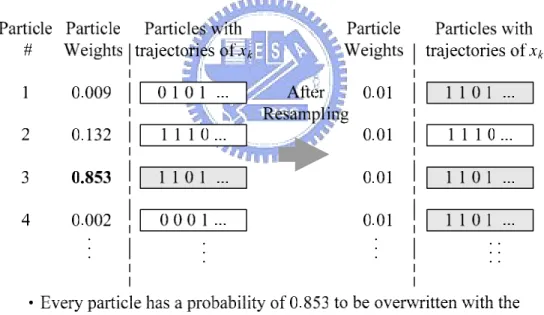
Fig. 1-1 Illustration of resampling (when Ns = 100)...15

C

HAPTER

2

Fig. 2-1 The system model...18

Fig. 2-2 Illustration of Log SIS sampling mechanism ...23

Fig. 2-3 Illustration of Max-Log SIS approximating Log SIS with different γ ...25

Fig. 2-4 Illustration of line of sight in communication systems ...27

Fig. 2-5 Illustration of the idea of delayed-sampling ...28

Fig. 2-6 Illustration of the idea of minimum phase filtering method ...30

Fig. 2-7 System diagram of the SIS based decision feedback equalization ...30

C

HAPTER

3

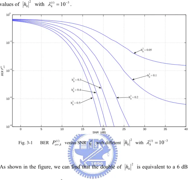
Fig. 3-1 BER P_err(i)_,k versus SNR ζ with different h₀2 as λ(_ki) =10−3...34

Fig. 3-2 BER P_err(i)_,k versus SNR ζ with different h₀2 as λ_k( )i =0.1...35

Fig. 3-3 Convergence trajectory of P_err(i)_,k as h₀2 = 0.2, SNR = 15 dB. ...37

Fig. 3-4 Convergence trajectory of P_err(i)_,k as h₀ 2 = 0.6, SNR = 15 dB...37

Fig. 3-5 Convergence trajectory of P_err(i)_,k as h₀ 2 = 0.36, SNR = 15 dB...38

Fig. 3-6 System model of the ZF-DFE...39

Fig. 3-7 System model of the MMSE-DFE ...44

C

HAPTER

4

Fig. 4-1 Block diagram of the adaptive filter algorithm...50

Fig. 4-2 System diagram of the SIS based adaptive DFE. ...52

Fig. 4-4 Illustration of information transmission between i-th PF and adaptive filter. ..55 Fig. 4-5 Implementation of the Max-Weight blind PF DFE. ...57

C

HAPTER

5

Fig. 5-1 BER versus SNR plots of the three equalizers under channel with a strong LOS. (Perfect CSI) ...61 Fig. 5-2 BER versus SNR plots of the SIS EQ under channel with different LOS.

(Perfect CSI) ...62 Fig. 5-3 BER versus SNR plots of the three equalizers under channel with weak LOS.

(Perfect CSI) ...63 Fig. 5-4 Comparison of BER versus SNR plots of the D-SIS EQ with different delay d

under channel with weak LOS. (Perfect CSI) ...64 Fig. 5-5 BER versus SNR plots of the different blind equalizations under channel with strong LOS ...67 Fig. 5-6 BER versus SNR plots of the three blind equalizations under channel with weak

LOS. ...67 Fig. 5-7 BER versus SNR plots of the four different blind equalizations under channel

1 I

NTRODUCTION TO

P

ARTICLE

F

ILTERING

T

HEORY

1.1 I

NTRODUCTION

Particle filter is a novel optimal filtering algorithm based on the Bayesian formulation and the sequential importance sampling (SIS) technique. It is basically one of the sequential Monte Carlo (MC) methodologies. The particle filter employs discrete random measures to recursively compute and to approximate the desired probability distributions. As a simulation-based algorithm, particle filtering is particularly useful in dealing with nonlinear and non-Gaussian problems, in which it is typically impossible to obtain the desired statistical estimates or distributions by using the traditional methods.

The sequential Monte Carlo methods like particle filtering were invented decades ago. However, they did not cause much attention because of the high computation complexity. The recent advances in digital circuit technologies make high-bandwidth computation possible and are able to put the MC methods into practice. Therefore the research of these topics has become active and attractive again recently. The SIS algorithm and the particle filtering theory have been discussed in detail in some previously published papers, as references [1] [2]. In this chapter, we will first bring out the motivation of this thesis, and then give a brief introduction on the particle filtering theory. The applications of equalizations using particle filtering are main topics of this thesis and will be discussed in the next chapters.

1.2 M

OTIVATION

There have been many articles discussing about the particle filtering equalization. However, rare of them addressed about the mathematical analysis of its bit error rate (BRE) performance. In sight of this, we would like to derive the BER of a particle as

a mathematic equation, and then analyze its behavior in the first part of this thesis. Besides, followed by the BER analysis of the particle filter equalizer, we can soon discover that its performance decays greatly under channels with an attenuated line of sight (LOS). As also discussed in the reference [3], this problem can be alleviated by the method of the delayed sequential importance sampling (D-SIS). The D-SIS algorithm, however, has some limitations and the notorious complexity issue in practical. This gives us some motivation to bring up an alternative solution that utilizes the minimum-phase pre-filtering to maximize the LOS of the equivalent channel.

1.3 F

UNDAMENTALS OF THE

P

ARTICLE

F

ILTERING

T

HEORY

The particle filtering is basically a suboptimal approach to perform Bayesian filtering. Consider the following state-space model,

x_k = f_k(x_k−1, )u_k (1-1) y_k =h_k( , )x n_{k k} (1-2) where u_kis the input vector, y_k is a vector of observations, x_k is the state vector,

( )

k

f ⋅ is the system transition function, ( )h_k ⋅ is the measurement function, and n_k

is the noise vector. Equation (1-1) is known as the state equation, and equation (1-2) is the measurement equation. Note that ( )f_k ⋅ and ( )h_k ⋅ are possibly nonlinear functions. In many signal processing applications, we are interested in the way of recursively computing the posteriori distribution p x

(

_k:0 y_k:0

)

1_{. To recursively} compute the posteriori probability, we can consider the following decomposition (see [2]):

(

k:0 k:0

)

(

k k 1

) (

k k:0

) (

k 1:0 k 1:0

)

p x y ∝ p x x ₋ ⋅p y x ⋅p x ₋ y ₋ (1-3) 1 _Here

{

}

:0 0, ,...,1 k = k

y y y y is a set of observation vectors. We would use this form to represent a sequential set of symbols or vectors in different time indices throughout this article.

The Bayesian filtering is stated as the ways of analytically computing these kinds of distributions in the close forms. Unfortunately, the analytic solutions (known as Kalman filter [1]) to the transition from p

(

x_k−1:0 y_k−1:0

)

to p x

(

_k:0 y_k:0

)

exist only in a

very restricted set of cases (e.g. when the systems are linear and the noises are Gaussian distributed). Therefore the particle filtering method has become an important alternative when we are solving nonlinear and non-Gaussian problems. When the particle filter is used, the distributions are approximated by discrete random measures via the Monte Carlo method. The random measures are composed of numerous particles which are samples drawn based on an estimated probability density function of the particles. The state space, and the weights are computed by using the Bayes theory. They are used to represent the “probability mass” of the particles. By the concept of Monte Carlo, the interested distribution ( )p x can be approximated as ( ) ( ) 1 ˆ ( ) ( ) s ( ) N i i i p x p x w δ x x = ≈ =

∑

⋅ − (1-4)

where _{x is the i-th particle,}( )i _{w is its weight, and} ( )i s

N is the number of the particles used in the approximation. It can be shown that as N_s → ∞ , the approximation approaches p x . ( ) δ

( )

⋅ is the Dirac delta function, i.e._{δ(x x−} ( )i _{) 1=}

if _{x x=} ( )i _{, and δ(x x−} ( )i _{) 0= , otherwise. As shown in [9], this kind of Monte Carlo}

approximation has a certain advantage: the computations of expectations involving complicated integrations are now simplified as summations. Particle filtering is simply a simulation-based Monte Carlo method to solve the sequential Bayesian problems by the approximation in (1-4).

The key concept in constructing the weights and the particles of particle filtering is the importance sampling principle. In the process of drawing particles, it is often

not possible to draw the samples directly from the desired distribution ( )p x . Therefore we have to generate particles from another distribution ( )q x , which is also known as the importance function. The un-normalized weights are assigned as follows,

( ) ( ) ( ) i k p x w q x = (1-5)

The weights are obtained after normalization:

( ) ( ) ( ) 1 , 1,2,..., i i k k N _j s k j w w i N w = = ∀ =

∑

(1-6)

The selection of the importance function ( )q x plays a crucial role in determining the performance of the particle filter. In general, the closer the importance function is selected to the desired distribution, the better the performance would be. A good choice of importance function can also reduce the effect of the degeneracy problem, which will be discussed in the next section. There are two most frequently used importance functions in the particle filtering applications: the priori importance function and the optimal importance function. The priori one is much easier for implementation while the optimal importance function minimizes the variance of the importance weights conditional on the trajectory of transmitted signal and the observations. The detail of the selection of the importance function is discussed in [8]. We would adopt the optimal importance function for analysis and simulations throughout this thesis.

To sequentially and recursively compute the importance functions and the particle weights, we need to update the weights and the importance function of each particle at every time slot through the equations as (1-3). The resulting method is referenced to the sequential importance sampling (SIS) algorithm. The detailed theory of the SIS algorithm can be found in many articles like [1] and [8]. We will discuss some important issues about the particle filtering in the following sections.

1.4 R

ESAMPLING

One major problem of the particle filtering is the degeneracy problem, which has been addressed in many previous articles like [1], [2] and [8]. It has been shown (as in [11] and [12]) that the variance of the importance weights can only increase over time due to propagation. Most of the particles will have negligible weights (very close to zero) after a few iterations. That is, much computation would be devoted in vain, The performance of the particle filter will become worse after a few interations. However, this problem can be alleviated by a good choice of the importance sampling function and resampling.

The idea of resampling is to elimiate the particles with negilible weights and replicate the largely-weighted particles. During the resampling, the larger weight a particle has, the more propable its particle (trajectory) would be replicated and overwrites the others. Each particles, after being re-allocated , would be given the same weight and then proceed the particle filtering process. In this article, the resampling is conducted whenever the effective sample size of the particle filter goes below a threshold ε. The effective sample size is defined as:

( ) 1 var( ) s eff i s k N N N w = ≤ + In practical, we estimate N with _eff

( )

_{( )} 2 1 1 s eff _{N i} s k i N N w = ≅ ≤

∑

The effective sample size can roughly represent the number of particles with weights that are not negilible (or, say, the particles that are still effective). The procedure of resampling is summarized as the following:

if (N_eff ≤ε), then

1. Replicate a new set of particles ~x_k(i) = x_k(i), for all i.

2. For each i, the i-th particle is assigend to the value of particle j with probability ( j) k w , i.e. () ~(j) k i k x x = with probability ( j) k w . 3. Normalize/re-assign the particle weights _k( )i 1

s

w N

= , for each i.

end if

Finally we give an example in Fig. 1-1, illustrating how the resampling works during the particle filtering.

1.5 P

RACTICAL

A

PPLICAIONS AND

L

IMITATIONS OF

P

ARTICLE

F

ILTERING

Particle filtering has been demonstrated as a powerful and promising methodology with a great range of applications in science and engineering. Within the field of communications, particle filtering has been widely applied to solve the channel equalization problems, including blind equalization, blind detection over flat fading channel (as addressed in [2]), and multi-user detections (MIMO) [13][14].

Nevertheless, as proposed in many articles like [3], particle filtering equalization suffers from performance decay under channels with a much attenuated line of sight (LOS), i.e. the first channel impulse response (CIR) is weak. To improve the performance under these channels, some solutions have been proposed. One of them is the method of delayed sequential importance sampling with resampling (D-SIR) proposed in [3], which incorporates the future observations to compute each particle at present. This method, however, requires the knowledge of the position of the largest impulse in CIR. Furthermore, the performance improvement of the D-SIR is achieved at the expense of the computational complexity, which is exponentially increased in proportional to the delay d. A large delay would lead to a great computational complexity which is nearly impractical.

Hence in this thesis we come out with a novel method that employs the idea of minimum phase filter implemented with the decision feedback equalizations (DFE) scheme. Instead of the idea to incorporate the future observations, we are considering to move the largest pulse in the CIR to the first one by employing the minimum energy-delay property of the minimum phase filter. This can be done by pre-calculated feedforward and feedback filter coefficients when the channel is known or by utilizing the adaptive filtering techniques (the least-mean-square (LMS) or the recursive least-squares (RLS) algorithms) when the channel is unknown.

1.6 T

HESIS

O

RGANIZATION

In Chapter 2 and Chapter 3, we would propose a particle filtering equalization scheme and analyze its bit error rate (BER) performance mathematically in the first part of this paper. And in the second part we come out with a new idea to keep good performance of the particle filtering under channel with attenuated LOS by applying minimum phase pre-filter followed by the particle filter. We verify the improvement of this method with mathematical prooves and give some comments at the end of Chapter 3.

Next we put this idea into practice in Chapter 4 as a realization of particle filtering blind equalizations. We propose the system diagram of the SIS-based blind and adaptive equalizers. In sight of the complexity of the blind particle filter equalizer (PF EQ), we further induce the method of Max-Weight PF EQ, which can greatly reduce the computation and system complexity.

In Chapter 5 we utilize the computer simulations to verify the inference and conclusions in Chapters 3 and 4. Finally we make the thesis conclusion and present the future works in Chapter 6. The appendixes and the references are provided at the end of this thesis for further information and consultation.

2 P

ARTICLE

F

ILTERING FOR

C

HANNEL

E

QUALIZATION

The main topics of this thesis are the performance and problems of the particle filter applied to equalization in the communication systems. In this chapter we first introduce the signal model and the SIS algorithm for equalizations. Then we discuss the problems and solutions of particle filter when the fading channels have a weak light-of-sight transmission path.

2.1 S

YSTEM

M

ODEL OF THE

P

ARTICLE

F

ILTER

E

QUALIZER

Consider a digital communication system where the BPSK symbols

}

{

1 , 0,1,2,...

k

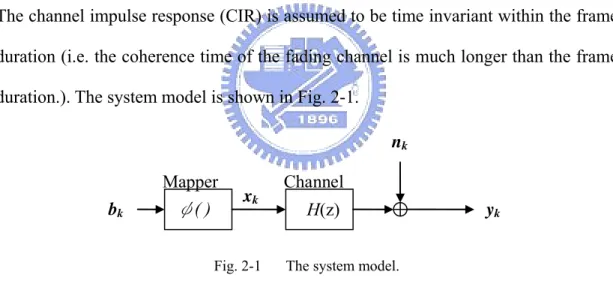
b ∈ ± k= are transmitted to a frequency-selective multi-path channel. The channel impulse response (CIR) is assumed to be time invariant within the frame duration (i.e. the coherence time of the fading channel is much longer than the frame duration.). The system model is shown in Fig. 2-1.

yk ψ( ) bk H(z) nk Mapper Channel xk

Fig. 2-1 The system model.

The transmitted bit stream b_k is mapped into x_k by using the BPSK mapping functionψ( ) as illustrated in Table. 2-1.:

k b 0 1 ) ( _k k b x =φ ＋A －A

The CIR is assumed to be finite-length and has M tap weights: {h₀,h₁,...,h_M−1}. For simplicity, the CIR is normalized to have unity power, i.e.

∑

M_l=0−1h_l 2 =1. The channel noise n_k is assumed to be additive white Gaussian noise (AWGN) with zero mean and the varianceσ , i.e._n2 n_k ~ Ν(0,σ_n2). Thus the discrete-time sequence of observations can be written as:

1 0 M k k l l k l y − x h₋ n = =

∑

+ (2-1)

We can now model the transmission by modifying the state-space formulation in (1-1) and (1-2) as follows: k k k Gx u x = ₋₁+ equation) (state (2-2) k k H k n y =h x + equation) on (observati (2-3)

where the M × 1 vector x_k =

[

x_k,x_k−1,…,x_k−M+1

]

T is the system state at symbol k, and , , ,h=

[

h h_{0 1} … h_M−1

]

T: M × 1 is the CIR vector. G is the M × M state-transition matrix: ⎥ ⎦ ⎤ ⎢ ⎣ ⎡ = × − − − × 1 1 1 1 1 0 M M M 0 I 0 G such that

[

] [

]

T M k k T M k k k x x x x x ₋₁, ₋₂ , ₋ = 0, ₋₁, , _{− +1} ⋅ … … G , and

[

]

T k k = x ,0,…,0 u is an

M × 1 vector of inputs. Our goal is to estimate the transmitted symbols x_k

recursively from the observations y_k. The optimum estimate of x_k is given by the maximum likelihood (ML) estimate (or MAP, if x_k is sent equally likely). However, it is not possible to compute the posteriori probability p

(

x_k:0 y_k:0

)

in the close form if the noise is non-Gaussian or the system is non-linear. Instead of using the complicated optimal solution, we are seeking the sub-optimal way, in which the approximation of posteriori probability p

(

x_k:0 y_k:0

)

is recursively computed with the

aid of sequential importance sampling (SIS) algorithm.

2.2 T

HE

SIS-

BASED

E

QUALIZATION

The optimal blind equalization is achieved by MAP detection of the transmitted sequence x , given the observations_k:0 y . Let _k:0 p

(

x_k:0 y_k:0

)

denote the posteriori probability mess function (p.m.f.) of the data sequence given the observations, The MAP algorithm is to find the estimated data sequence that maximizes this posteriori probability. The most straightforward way of finding the MAP solution is to exhaustedly compute the probabilities of all 2k+1 possible x and select the largest ˆ_k:0 one. However, this is impractical due to the high computation complexity. It is preferable to find the estimate MAP

k 0:

ˆx that maximizes the posteriori p.m.f. from the

previous estimate MAP k 1:0

ˆ ₋

x recursively even thought the final solution is sub-optimal. To recursively compute the posteriori probability, we utilize the decomposition in (1-3) of Chapter 1:

(

k:0 k:0

) (

∝ p xk xk−1

) (

⋅p yk k:0

) (

⋅ p k−1:0 k−1:0

)

p x y x x y (1-3)

Assume that the data bit b_k is uncorrelated with the bit b_lat the different time l , k≠ l., i.e. p

(

x_k x_k−1

)

= p

( )

x_k . Using the similar derivation in [3], we can obtain the

likelihood function:

(

)

⎟⎟ ⎟ ⎠ ⎞ ⎜⎜ ⎜ ⎝ ⎛_{− −} = ₂ 2 0 : 2 exp 2 1 n k H k n k k y y p σ σ π x h x (2-4)

From the equations (1-3) and (2-4), we can find a recursive equalization algorithm by computing the posteriori p.m.f. p

(

x_k:0y_k:0

)

sequentially.

According to the particle filtering theory in Chapter 1 and [1, 2], we want to draw Ns particles x ik( )i , =1,2,...,Ns from an importance function q

(

xk:0yk:0

)

and

give them the weights based on the true posteriori probabilityp

(

x_k:0 y_k:0

)

:

(

k

)

i k i k i k q x y x ~ () , 0 : 1 ) ( ) ( − x (2-5)

(

) (

)

(

k

)

i k i k i k k i k i k i k i k y x q y p x x p w w , ) ( 0 : 1 ) ( ) ( 0 : ) ( 1 ) ( ) ( 1 ) ( − − − ⋅ ⋅ ∝ x x (2-6)

The importance function q

(

x_k:0y_k:0

)

is the trial p.m.f. which approximates

(

k:0 k:0

)

p x y . It is easier to draw samples from q

(

x_k:0y_k:0

)

than p

(

x_k:0 y_k:0

)

. The adaptation of the normalized weight (2-6) is derived from (1-3) and the following factorization of importance function:

(

k:0 k:0

) (

∝q xk k−1:0,yk

) (

⋅q k−1:0 k−1:0

)

qx y x x y (2-7)

The Ns particles constitute a Monte Carlo smoother (MC smoother) that approximates

the true posteriori p.m.f. for each time slot k:

( ) ( ) :0 :0 :0 :0 :0 :0 1 ˆ ( ) ( ) s ( ) N i i k k k k k k k i p p w δ = ≈ =

∑

⋅ − x y x y x x (2-8) where () 0 : i k

x are the particles, (i)

k

w are their weights and δ

( )

⋅ is the Dirac delta function.

There are many choices to decide the importance sampling function q

(

x_k:0 y_k:0

)

,. Here we choose the optimal importance function that collects all available information up to time k . ) ( ) ( ) , ( ) , ( ) , ( ) ( 0 : 1 ) ( 0 : 1 ) ( 0 : 1 ) ( 0 : 1 ) ( 0 : 1 i k k i k k i k k k k i k k k i k k y p x p x y p y x p y x q − − − − − ⋅ = = x x x x x (2-9)

Substituting (2-9) into (2-5) and (2-6), we have

) ( ) , ( ) ( ) , ( ) ( ~ ₍₎ 0 : 1 ) ( 0 : 1 ) ( ) ( x x p x x y p x p x y p P x k ion constellatx i k k k k i k k k i k i k = = = ⋅ = ≡

∑

∈ ∀ − − x x χ χ χ (2-10)

) ( ) , ( ) ( () ()_1:0 1 ) ( 0 : 1 ) ( 1 ) ( k x i k k k i k i k k i k i k w p y w p y x p x w k

∑

⋅ ⋅ = ⋅ ∝ ₋ x _{− −} x ₋ (2-11)

If the channel is known, the estimate of the likelihood function for the i-th particle at time k is

(

( )

)

( ) 2 1:0 2 1 ˆ , exp 2 2 H i k k i k k k n n y p y x χ σ πσ − ⎛_{− −} ⎞ ⎜ ⎟ = = ⎜ ⎟ ⎝ ⎠ h x x _{((22--1122) )} where

(

i

)

T M k i k i k i k x x x ) ( 1 ) ( 2 ) ( 1 ) ( _{, , ,...,} ~ + − − − = χ

x , and χ is the drawn sample for testing (i)

k

x . To draw samples for a particle according to the likelihood function (2-10) and put the SIS algorithm into practice, we propose two algorithms here for sample drawing of each particle.

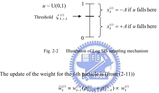
2.2.1 Log SIS

From the definition of (i)(_χ)

k

P in (2-10) and the fact thatχcould be either +A or

－A. We can determine a sample drawing mechanism that employs a uniformly distributed random variable (r.v.) u ~ U(0,1) to draw samples for (i)

k

x . Since the denominator of (i)(_χ)

k

P is the same whenχ =+Aor −A, we consider only the numerator. Define () , ) ( , & ki A i A k+ ρ − ρ as the numerator of (i)(_χ) k P whenχ = +A and − , respectively: A

) ( 2 exp 2 1 ) ( ) , ( 2 2 1 1 ) ( 0 ) ( 0 : 1 ) ( , A x p x h h A y A x p A x y p k n M l i l k l k n k i k k k i A k + = ⋅ ⎟ ⎟ ⎟ ⎠ ⎞ ⎜ ⎜ ⎜ ⎝ ⎛_{− − ⋅ − ⋅} = + = ⋅ + = ≡

∑

− = − − + σ σ π ρ x (2-13) and similarly ) ( 2 exp 2 1 2 2 1 1 ) ( 0 ) ( , p x A x h h A y k n M l i l k l k n i A k ⋅ =− ⎟ ⎟ ⎟ ⎠ ⎞ ⎜ ⎜ ⎜ ⎝ ⎛_{− + ⋅ − ⋅} =

∑

− = − − _σ σ π ρ (2-14)

By normalizing () , ) ( , & i A k i A k+ ρ −

ρ , we can determine a threshold () , i A k+ ζ ) ( ) ( () () , ) ( , ) ( , ) ( , P A i k i A k i A k i A k i A k+ ≡ρ + ρ + +ρ − = + ζ (2-15)

so that if the uniform r.v. u falls in the interval

[

()

]

,

, 0 i

A k+

ζ , then the particle (i)

k

x is assigned as +A, and vice versa. The way of generating the i-th particle (i)

k x at time k is illustrated in Fig. 2-2. 0 1 Threshold (,) i A k+ ζ u ~ U(0,1) here falls if ) ( _{A u} x i k =− here falls if ) ( _{A u} x i k =+

Fig. 2-2 Illustration of Log SIS sampling mechanism

The update of the weight for the i-th particle is (from (2-11))

) ( ) ( , ) ( , ) ( 1 ) ( _{( )} ~ i k i A k i A k i k i k w w w ≡ ₋ ρ ₊ +ρ ₋ ∝ (2-16) where ~(i) k

w it the weight before normalization, and the new weight (i)

k

w of i-th particle at time k can be obtained after the normalization:

( ) ( ) ( ) 1 , 1,2,..., s i i k k N _j s k j w w i N w = = ∀ =

∑

(2-17) 2.2.2 Max-Log SIS

In this section we want to further simplify the computation of the threshold by using some approximations. Let us look at the definition of ()

, i A k+ ζ in (2-15). Since ) ( , ) ( , & ki A i A k+ ρ −

ρ are composed of exponential terms, we can obtain the new threshold

) ( , i A k+

the denominator of the original threshold:

(

)

(

)

( ) , ( ) , ( ) ( ) , , ( ) , ( ) ( ) ( ) ( ) , , , , ( ) ( ) , , ( ) , ( ) ( ) , , ( ) ( ) , , ( ) exp( ) 1 1 exp ( ) , if exp( ) exp( ) exp( ) exp ( ) exp( ) exp( ) i k A i k A i i k A k A i k A i i i i k A k A k A k A i i k A k A i k A i i k A k A i i k A k A ρ ζ ρ ρ α _{α α ρ ρ} α α α α α α α + + + − − − + + − + − + − + + − ≡ + − − = − − − > − + − = − = − − − + − ( ) ( ) , , , if i i k A k A ρ ₊ ρ ₋ ⎧ ⎪ ⎪ ⎨ ⎪ _≤ ⎪ ⎩

Thus we have simplified the computation of the threshold as

(

)

(

)

( ) , ( ) ( ) ( ) ( ) , , , , ( ) , ( ) , _{( )} , ( ) ( ) ( ) ( ) , , , , ( ) , 1 =1 exp , if = exp , if i k A i i i i k A k A k A k A i k A i k A _i k A i i i i k A k A k A k A i k A ρ α α ρ ρ ρ ζ ρ α α ρ ρ ρ − + − + − + + + + − + − − ⎧ − − − − > ⎪ ⎪ ≅ ⎨ ⎪ _{− − ≤} ⎪ ⎩ ( ) ( ) ( ) ( ) , , , ,

where log(i i ), i log( i )

k A k A k A k A α ₊ = − ρ ₊ α ₋ = − ρ ₋ . If (p x_k = +A)= p x( _k = −A), then ( ) , i k A α ₊ and ( ) , i k A

α ₋ can be simplified as the exponent term of ( ) , i k A ρ ₊ and ( ) , i k A ρ ₊ : 2 1 ( ) ( ) , 0 ₁ M i i k A yk A h _l h xl k l α ₊ = − ⋅ −

∑

₌− ⋅ ₋ 2 1 ( ) ( ) , 0 ₁ M i i k A yk A h _l h xl k l α ₋ = + ⋅ −

∑

₌− ⋅ ₋

To reduce the error produced by this approximation and to make the new threshold closer to the original one, we generalize the ratio of ()

, ) ( , ki A i A k+ ρ − ρ or () , ) ( , ki A i A k− ρ + ρ as ( ) ( ) ( ) , , 1 exp( ), 0 2 i i i k k A k A ρ = −γ α ₊ −α ₋ γ >

with the parameter γ to give some exponential weighting on it. The effects of this parameter would be discussed later in this section. Now we can define the threshold

) ( , i A k+

ψ for the Max-Log SIS as:

⎩ ⎨ ⎧ ≤ > − ≡ − + − + + if , if , 1 ) ( , ) ( , ) ( ) ( , ) ( , ) ( ) ( , i A k i A k i k i A k i A k i k i A k _{ρ ρ ρ} ρ ρ ρ ψ (2-18)

We can see that in both cases, () ,

i A k+

ψ would approach to (i) A k,

properly. To further illustrate that the Log SIS algorithm can be approximated by the Max-log SIS, we plot (i)

A k, ζ ₊ and () , i A k+ ψ as functions of (

∑

₁−1 () ) = ⋅ − − _lM i l k l k h x y in Fig.

2-3. with different values of γ .

) (

∑

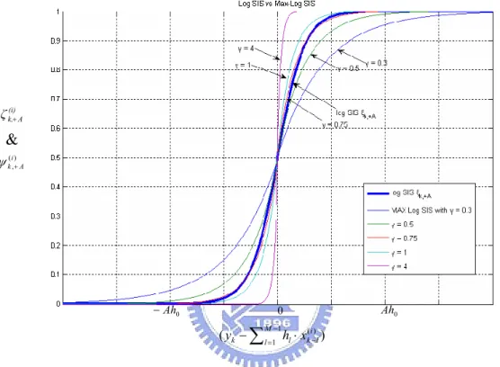
₁−1 () = ⋅ − − M l i l k l k h x y 0 Ah − 0 Ah0 (i) A k, ζ + & ) ( , i A k+ ψ

Fig. 2-3 Illustration of Max-Log SIS approximating Log SIS with different γ

We can observe that () , i A k+ ψ approaches (i) A k, ζ ₊ as γ is around 0.75. As γ increases, the characteristic function of ()

,

i A k+

ψ would approach to a step function,

which implies that the hard decision scheme is applied to draw sample for (i)

k

x . In this case, most of the particles would be drawn to be the same value at each time slot, and the particle filter can no longer compute the estimation of the desired posteriori probability. On the other hand, if we choose γ to be a very small value (e.g.

0.5 <

γ ), we can observe from Fig. 2-3 that even when

0 1 1 ) ( ₎ (y M_l h x i A h l k l k −

∑

⋅ > ⋅ −

is still quite a little probability that the particles would be drawn wrongly, and the error probability would increase.

Similarly, if we define _log(( )i ( )i _{) and log(}( )i ( )i ₎

k k k k

W = w W = w , we can take

logarithm and apply Jacobian approximation to the weight (i)

k

w (2-16) and (2-17). We can obtain the following weight adaptation for Max-Log SIS:

( )

(

)

(

)

( ) ( ) ( ) ( ) 1 , , ( ) ( ) ( ) 1 , , ( ) ( ) ( ) 1 , , log log log max( , ) min( , ) (2 -19) i i i i k k k A k A i i i k k A k A i i i k k A k A W w W W ρ ρ ρ ρ α α − + − − + − − + − ≡ + + = + = −

Similar to the Log-SIS case, the normalized weights would be:

( ) ( ) ( ) 1 log( N ), 1, 2,..., (2 - 20) i i j k k _j k W =W −

∑

₌ w ∀ =i N

These logarithm SIS algorithms have an addition advantage on the implementation. Consider the case when the likelihood function is too small. The value may be truncated and may not be stored accurately due to the finite precision problem caused by limiting number of bits in a word. By utilizing the logarithms we can avoid these undesired truncations caused by insufficient bits.

2.3 P

RACTICAL

I

SSUE

—

P

ROBLEM AND

S

OLUTIONS OF

SIS

EQ

UNDER WEAK

LOS

CHANNELS

As we have mentioned in Chapter 1, the particle filter based equalization encounters a performance loss under the channel with a much attenuated line of sight (LOS)2.

Tx

Rx Line of sight

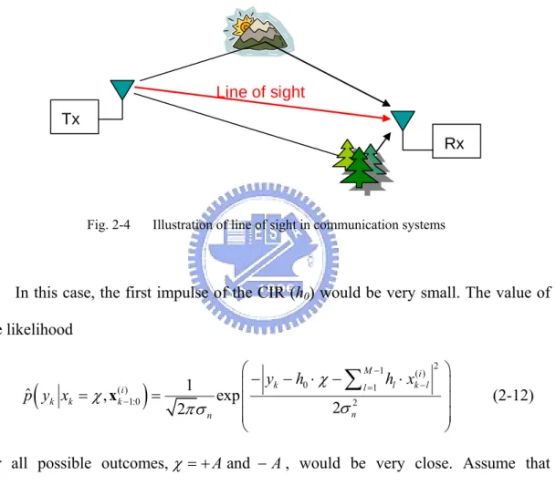
Fig. 2-4 Illustration of line of sight in communication systems

In this case, the first impulse of the CIR (h0) would be very small. The value of

the likelihood

(

)

2 1 _{( )} 0 1 ( ) 1:0 2 1 ˆ , exp 2 2 M _i k l l k l i k k k n n y h h x p y x χ χ σ πσ − − = − ⎛_{− − ⋅ − ⋅} ⎞ ⎜ ⎟ = = _{⎜ ⎟} ⎜ ⎟ ⎝ ⎠

∑

x (2-12)

for all possible outcomes,χ = +A and − , would be very close. Assume that A symbols are sent equally likely, the difference between ( ) ( )

, and ,

i i

k A k A

ρ ₊ ρ ₋ , in (2-13) and

(2-14), , would be small so that the SIS algorithm can hardly determine (or draw out) the desired particle. Hence the symbols will be erroneously decided in the receiver, and the performance of the particle filter decreases.

2 _{Line of sight (LOS) is commonly used to refer to telecommunication links that rely on a line of sight}

directly between the transmitting antenna and the receiving antenna (as illustrated in Fig. 2-4), and its gain would usually be valued as the first impulse response of the CIR.

2.3.1 Delayed Sampling

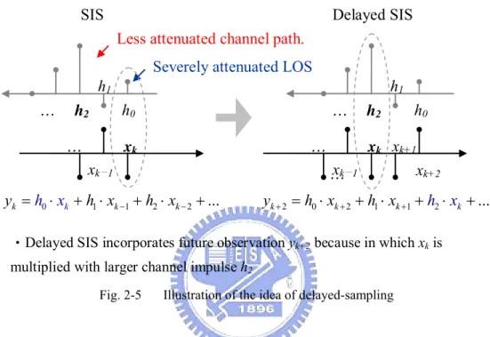
One strategy to overcome this problem is the delayed-sampling technique, proposed in [3]. The basic idea of the delayed-sampling algorithm is to utilize the possible large (un-attenuated) and lagged CIR pulses and enumerate the future observations to determine the present particle, as illustrated in Fig. 2-5.

Less attenuated channel path.

Severely attenuated LOS

1 1 2 2 0 ... k k k k y =h ⋅x + ⋅h x ₋ + ⋅h x ₋ + h0 h1 h2 … xk xk－₁ … 2 2 0 2 1 1 ... k k k k y ₊ = ⋅h x ₊ + ⋅h x ₊ +h x⋅ + … h0 h1 h2 … xk+2 xk+1 xk xk－₁

‧Delayed SIS incorporates future observation yk+2 because in which xk is

multiplied with larger channel impulse h2

…

Delayed SIS SIS

Fig. 2-5 Illustration of the idea of delayed-sampling

Note that the CIR in this figure is placed in reversed order to illustrate how the computations work in the convolution of h and x.

More specifically, the sampling of a particle ( )i k x is delayed until y_{k d+} is observed,

(

)

( ) ( ) ( ) 1:0 : ~ , i i i k k k k k d x q x x ₋ y ₊ (2-21)

(

) (

)

(

)

( ) ( ) ( ) 1 : :0 ( ) ( ) 1 _{( ) ( )} 1:0, : i i i k k k k d k i i k k _{i i} k k k k d p x x p w w q x − + − − + ⋅ ∝ ⋅ y x x y (2-22)

Compared with the original SIS algorithm (2-10) and (2-11), the particles are now drawn from the delayed importance p.m.f. and the weights are updated accordingly. The likelihood function now becomes

(

)

(

)

(

1:

)

1: ( ) ( ) : 1:0 : 1: 1:0 { 1} ( ) : 1: 1:0 { 1} ˆ , ˆ , , ˆ , , d t t d d t t d i i k k d k k k k d t t d k k s i k k d t t d k k s p x p x x p x x χ χ χ + + + + + − + + + − ∈ ± + + + − ∈ ± = = = ∝ =

∑

∑

y x y x y x (2-23)

Again, the proportionality comes from the assumption that the transmitted symbols are sent equally likely.

The delayed-SIS algorithm, however, has some limitations. First, as depicted in Fig. 2-5, it is straightforward that the delay d needs to be large enough to cover the less attenuated CIR. This requires the knowledge of the channel delay, which is usually unknown in the blind equalization scenarios. In addition, the computational complexity of the delayed-SIS algorithm has been increased exponentially because of the marginalization of all possible outcomes as shown in (2-23). Furthermore, the performance of the delayed-SIS method is not necessarily growing with the delay d (we will illustrate this in Chapter 5). In other words, it is possible that the performance decays when the delay d increases. The computation spent for the extra delay would be in vain. This usually happens when the delay d is larger than the channel length. In this situation, all of the information given in (2-23) would be the future symbols x_{t+ +1:t d}, and none of the previous particles would be applied in this computation. The particle filter loses its function to storage the discrete measures.

2.3.2 Minimum Phase filter Solutions

As discussed in the previous section, the delayed-SIS has some limitations and high computation complexity. Here we will propose a novel particle filtering scheme, which utilizes the minimum phase filters implemented in the form of decision feedback equalizations (DFE). As introduced in many digital signal processing textbooks, the minimum phase system has the property that the partial energy is most concentrated at the first impulse of the impulse response h(n) (the minimum energy delay property [sec. 5.6.3 [7]]). The idea of this method is illustrated in Fig. 2-6.

CIR with an attenuated LOS 0 1 1 2 2 ... k k k k y = ⋅h x + ⋅h x ₋ + ⋅h x ₋ + h0 h1 h2 … xk xk－1 … 0 1 1 2 2 ... k g k g k k y = ⋅x + ⋅x ₋ +g ⋅x ₋ + g0 g1 g2 …

‧After the minimum phase pre-filtering, the equivalent channel would have a large first impulse, and therefore xk would by multiplied with a larger LOS g0.

Equivalent CIR after DFE (reversely ordered)

xk

xk－1

…

SIS SIS with minimum phase pre-filter

Fig. 2-6 Illustration of the idea of minimum phase filtering method

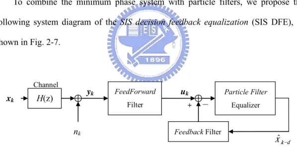
To combine the minimum phase system with particle filters, we propose the following system diagram of the SIS decision feedback equalization (SIS DFE), as shown in Fig. 2-7. H(z) nk Channel xk yk FeedForward Filter Feedback Filter + － uk Particle Filter Equalizer d k xˆ ₋ Fig. 2-7 System diagram of the SIS decision feedback equalization

The match filter cascaded with a noise whitening filter forms a feedforward filter (FFF). The feedback filter (FBF) is a minimum phase filter. In the case of known channel state information (CSI) in the time-invariant system, the coefficients of the FFF and FBF can be pre-calculated under the criteria of zero-forcing (ZF) or minimum mean square error (MMSE). When the channel information is unknown or varies with time, the adaptive filtering techniques such as RLS or LMS can be applied to fulfill

the operation of blind equalization. The details of the SIS based ZF and MMSE DFE would be introduced in the next chapter, and the implementation of blind equalization with adaptive filtering would be discussed in Chapter 4.

2.4 C

HAPTER

S

UMMARY

In this chapter, we have briefly introduced the particle filtering equalization structure, and conceptually explained why channels with a weak LOS would reduce the performance of a particle filtering equalizer (PF EQ). To solve the weak LOS problem, we propose the SIS decision feedback equalization structure. Based on the defined notations and models, we will provide the detailed mathematical analysis of its bit error rate in the next chapter. We will show the effects of the weak LOS problem and how the proposed SIS decision feedback equalization can solve this problem.

3 P

ERFORMANCE

A

NALYSIS OF

M

AX

-L

OG

SIS

E

QUALIZATION

A

LGORITHMS

In this chapter, we attempt to analyze the BER of the equalization system based on the Max-Log SIS algorithm. We will first derive the BER in 3.1 and further analyze the convergence behavior in 3.2. Then, we will focus on the performance analysis of the SIS decision feedback equalizers proposed in Chapter 2 and illustrate how they improve the performance (BER). Finally we will have a chapter summary in the end of the chapter.

3.1 D

ERIVATION OF THE BIT ERROR PROBABILITY

In the following analysis, we consider only the i-th particle and analyze the bit error rate (BER) of this particle. Assume that the data sequence bk are sent equally

likely, i.e. the priori probability p(b_k =0)= p(b_k =1)=1 2 . According to the Max-Log SIS algorithm, we can calculate the error probability of the i-th particle as:

( ) ( ) ( ) , 1 _{( ) ( ) ( )} , , , 0 1 _{( ) ( ) ( )} , , , 0 1 ( | ) ( ) ( | ) ( ) 1 1 ( , ) ( ) 2 1 ( , ) ( 2 i i i err k k k k k k k i i i k A k A k k A k i i i k A k A k k A k P p x A x A p x A p x A x A p x A p u x A p x A d p u x A p x ψ ψ ϕ ψ ϕ ϕ ψ ψ ϕ ψ ϕ + + + + − − = − = + = + ⋅ = + − = − = − ⋅ = − = − ⋅ ≤ = = + ⋅ = = + − ⋅ ≤ = = − ⋅ = = −

∫

∫

1 _{( )} 1 _{( )} , , 0 0 ( ) ( ) , , ) 1 1 1 ( ) ( ) 2 2 1 1 1 [ | ] [ | ] (3-1) 2 2 i i k A k k A k i i k A k k A k A d p x A d p x A d E x A E x A ϕ ϕ ψ ϕ ϕ ϕ ψ ϕ ϕ ψ ψ + − + − = − ⋅ ⋅ = = + − ⋅ ⋅ = = − = − = + − = −

∫

∫

where )u~ U(0,1 is a uniform distributed r.v. with the range [0,1]. Based on the calculation of [ () | 0]

,+ k = i A k b Eψ and [ () | 1] ,− k = i A k b Eψ (the details

are in Appendix B), we obtain the error probability () ,

i k err

2 2 ( ) ( ) ( ) , 0( , 0 , ) 1( , 0 , , ) i i i err k k k P =F λ h ζ +F λ h ζ γ _((33--22))

(

)

(

)

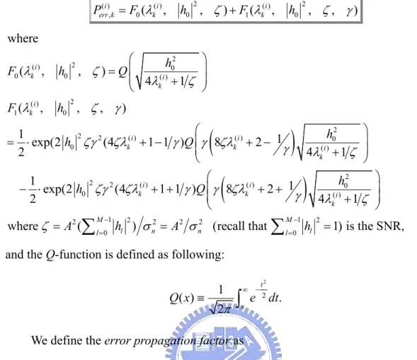
2 2 ( ) 0 0 0 ( ) 2 ( ) 1 0 2 2 _{2 ( ) ( ) 0} 0 ( ) 2 2 _{2 ( ) ( ) 0} 0 ( ) 2 where ( , , ) 4 1 ( , , , ) 1 ₁ exp(2 (4 1 1 ) 8 2 2 4 1 1 ₁ exp(2 (4 1 1 ) 8 2 2 4 1 where ( i k i k i k i i k k i k i i k k i k h F h Q F h h h Q h h Q A λ ζ λ ζ λ ζ γ ζγ ζλ γ γ ζλ _γ λ ζ ζγ ζλ γ γ ζλ _γ λ ζ ζ ⎛ ⎞ = ⎜_⎜ ⎟_⎟ + ⎝ ⎠ ⎛ ⎞ = ⋅ + − ⎜_⎜ + − ⎟_⎟ + ⎝ ⎠ ⎛ ⎞ − ⋅ + + ⎜_⎜ + + ⎟_⎟ + ⎝ ⎠ = 1 2 _{2 2 2} 1 2

0 ) (recall that 0 1) is the SNR,

M M l n n l l h σ A σ l h − − = = = =

∑

∑

and the Q-function is defined as following:

2 2 1 ( ) . 2 t x Q x e dt π − ∞ ≡

∫

We define the error propagation factor as

∑

− = − = 1 1 ) ( , 2 ) ( M l i l k err l i k h P λ

This factor indicates the error contribution of the previous BERs after the channel responses are applied.

In the rest of this section, we will observe the influence of all parameters on F0

and F1. The BER of the i-th particle at time k Perr(i),k is a function of the error

propagation factor ( )i k

λ , the power of the first CIR h , the SNR ₀2 ζ , and the Max-Log SIS parameter γ . To see the effect h on the performance, we choose ₀2

0.75

γ = and fix ( )i k

λ to observe the BER versus SNR graph with different values of

2 0

h .

Fig. 3-1 is the plot of () ,

i k err

values of h with ₀2 (i) ₌₁₀−3 k λ . 0 5 10 15 20 25 30 35 40 10−8 10−6 10−4 10−2 100 SNR (dB) BER P er r (i ) h₀2 = 0.05 h 0 2 _{= 0.1} h₀2 = 0.2 h₀2 = 0.3 h 0 2 _{= 0.4} h 0 2 _{= 0.5} Fig. 3-1 BER (), i k err

P versus SNR ζ with different h₀2 with λ(_ki) =10−3

As shown in the figure, we can find that the double of h is equivalent to a 6 dB ₀ 2

increase in SNR when h is sufficiently large. Therefore it is essential to make ₀ 2

2 0

h large enough to obtain acceptable low bit error rate. Note that this BER versus SNR plot is drawn under the condition that the error propagation factor ( )i

k

λ is fixed. In fact, when h is small, the value of ₀ 2 ( )i

k

λ would be increased because the error propagation may be enlarged by the rest impulses of the CIR. When ( )i

k

λ is increased to 0.1, the BER versus SNR plot would be as shown in Fig. 3-2.

−2 0 2 4 6 8 10 12 14 16 18 20 10−1 100 SNR (dB) BER P er r (i ) h 0 2 _{= 0.05} h₀2 = 0.3 h₀2 = 0.1 h 0 2 _{= 0.2} h₀2 = 0.4 h₀2 = 0.5 Fig. 3-2 BER (), i k err

P versus SNR ζ with different h₀2 as λ_k( )i =0.1

To evaluate the effects of ( )i k

λ on the performance is difficult because ( )i k

λ varies with time. However, our simulation results show the BER curves are similar to the lower curves in Fig. 3-1 when h is large and similar to the upper ones in Fig. 3-2 as ₀2

2 0

h is small.

3.2 C

ONVERGENCE BEHAVIOR OF THE AVERAGE

BER

OF A

P

ARTICLE

From (3-2) and the definition of (i)

k

λ , we can observe that () ,

i k err

P is a function of

the previous M-1 averaged bit error probabilities

{

() 1,2,..., 1

}

, − l= M −

P i l k

err . That is, the

averaged bit error probability of a particle may change with time. It is not easy to analyze the convergence behavior of ()

,

i k err

P when M is large. In general () ,

i k err

P will converge to stable equilibrium points, which are determined by the crossing points of a plane and a line in the hyper space (p₀,p₁,...,p_M−1) as the following.

2 ( ) ( ) 0 ,0 0 1 0 2 1 1 2

The hyper plane:

( , , , ) and the hyper lines:

i i err k M M p P h p p p p p p λ ζ γ − − = = ⎧ ⎪ ₌ ⎪ ⎨ ⎪ ⎪ ₌ ⎩

The negative going cross points correspond to stable equilibrium points whereas the positive going cross points correspond to unstable equilibrium points.

To illustrate the convergence of () ,

i k err

P , we observe the case M = 2 with different

values of h and plot the convergence trajectories of the ₀2 () ,

i k err

P as in Fig. 3-3, Fig.

3-4, and Fig. 3-5. The arrowed lines represent the convergence trajectories of () ,

i k err

P as

the time index k increases (k = 0, 1, 2 ...). We can see that in Fig. 3-3 and Fig. 3-4,

) ( , i k err

P will eventually converge to single stable equilibrium point E. In Fig. 3-5, when

2 0

h =0.36 (in the middle range), there are two stable equilibrium points (E0 and E1) and an unstable equilibrium point (U). If ()

0 ,

i err

P is initially located in the range I0,

) ( , i k err

P would eventually converge to E0. On the other hand, if () 0 ,

i err

P is initially

located in the range I1, () ,

i k err

P would eventually converge to E1, as shown in Fig.3-3.

The steady state () ,

i k err

P at E0 is much smaller that at E1. We call the initial point within

the interval I0 a good initial. How to make () 0 ,

i err

P fall in good initials is one of the important factors of obtaining good performance. That is actually the research topics we intend to study in the future. In addition, the unstable equilibrium point separate the convergence intervals I0 and I1.

Fig. 3-3 Convergence trajectory of (),

i k err

P as h₀2 = 0.2, SNR = 15 dB.

Fig. 3-4 Convergence trajectory of (),

i k err