無線區域網路之即時服務排程演算法

全文

(1)國立交通大學電子工程學系電子研究所碩士班碩士論文. 無線區域網路之即時服務排程演算法. Real-Time Services Scheduling Control Algorithm in WLAN. 研究生：范裕隆指導教授：黃經堯. 博士. 中華民國九十四年七月.

(2) 無線區域網路之即時服務排程演算法. Real-Time Services Scheduling Control Algorithm in WLAN 研究生: 范裕隆指導教授: 黃經堯. Student: YuLong Fan Advisor: Ching Yao Huang. 國立交通大學電子工程學系電子研究所碩士班碩士論文. A Thesis Submitted to Department of Electronics Engineering & Institute of Electronics College of Electrical Engineering and Computer Science National Chiao Tung University in partial Fulfillment of the Requirements for the Degree of Master of Science in Electronics Engineering. July 2005 HsinChu, Taiwan, Republic of China. 中華民國九十四年七月.

(3) 無線區域網路之即時服務排程演算法研究生:. 范裕隆. 指導教授: 黃經堯博士. 國立交通大學電子工程學系電子研究所碩士班. 摘要 IEEE 802.11 無線區域網路已發展多年，隨著服務品質的需求，IEEE 802.11e 根據原 IEEE 802.11 媒體存取控制層提出改良與增進的控制機制。無線區域網路的媒體存取機制可分成中央輪詢和分散競爭兩種：中央輪詢式媒體存取藉由一中央存取點(AP) 負責分配無線網路頻寬；在分散競爭的存取環境下，各使用者(Station)競取共享頻寬。本論文主要探討前者，除了介紹標準文獻所提出的簡單排程演算法外，尚提出一以計時器為基底之演算法。經由完整的模擬結果而有以下三結論：一，中央輪詢式存取的頻寬使用效率優於分散競爭而可支援較多的使用者；二，相較於平等對待每一個使用者的簡單排程演算法，所提出的演算法提供區別性服務，在單考慮即時服務下，可支援較多使用者外；在考慮即時與非即時服務下，亦可增加非即時服務傳輸流量；三，二演算法本身都具有可調整之交易(tradeoff)參數，本研究除模擬其影響並交互比較，其結果亦顯示出所提之演算法相較於簡單演算法之優越性。. i.

(4) Real-Time Services Scheduling Control Algorithm in WLAN Student: YuLong Fan. Advisor: Dr. Ching Yao Huang. Department of Electronic Engineering & Institute of Electronics National Chiao Tung University. Abstract With the growing QoS requirements in Wireless Local Area Network (WLAN), it is crucial to emphasize the enhanced Medium Access Control (MAC) layer in the 802.11e. This thesis adopts the centralized polling-based scheduler mechanism rather than the distributed contention-based channel access to allocate the precious shared resource for each service. Besides of pointing out the equal treatment of the simple scheduling algorithm for all kinds of services, this thesis proposes a timer-based scheduling algorithm which is based on the concept of the Earliest Deadline First to improve the bandwidth utilization and support the differentiate QoS demands. Based on the complete comparisons by the simulation, the polling-based mechanism is superior to contention-based access on the bandwidth efficiency,. which results in the higher capacity. Furthermore, the proposed. algorithm provides better bandwidth utilization than the simple algorithm in the capacity and the data throughput under the QoS requirements. In addition, the influence of the adjustable tradeoff parameter for each algorithm itself is revealed.. ii.

(5) Acknowledgement After the past two years, it is time to end the pleasure learning life at school. I am glad to meet all of you around my learning life. Without your supporting and guide, it would be boring and agonizing. At first, I want to acknowledge my advisor, Dr. Ching Yao Huang, for the sharing of the knowledge and experiences, the guiding of the concept and opinion. Different from the general spoon-fed education, he provides an open and heuristic method laboratory. Besides, I also appreciate my colleagues include all the members of the laboratory and my roommates, the cross and broad discussions show me the wide field of version and the accompanying prevents from the loneliness. Finally, I deeply thank my family for the long-term love and encouragement. This thesis is presented for you!. iii.

(6) Contents Chapter 1 Introduction........................................................................................ 1 1.1 Background.............................................................................................................. 1 1.2 QoS and Scheduler ................................................................................................... 2 1.3 Organization............................................................................................................. 4. Chapter 2 Medium Access Control of Wireless Local Area Network.................. 5 2.1 Architecture of Wireless Local Area Network........................................................... 5 2.1.1 Components................................................................................................... 5 2.1.2 Topologies ..................................................................................................... 7 2.2 802.11 MAC ............................................................................................................ 8 2.2.1 Distributed Coordination Function................................................................. 8 2.2.2 Point Coordination Function .........................................................................11 2.3 802.11e MAC......................................................................................................... 13 2.3.1 Enhanced Distributed Coordination Function............................................... 13 2.3.2 Hybrid Coordination Function ..................................................................... 16. Chapter 3 Scheduling Algorithms in WLAN .................................................... 18 3.1 Simple Scheduling Algorithm................................................................................. 18 3.2 Proposed Timer-Based Scheduling Algorithm......................................................... 20 3.3 Analysis of Algorithms’ Concept ............................................................................ 24. Chapter 4 Simulation Results ........................................................................... 26 4.1 Simulation Model................................................................................................... 26 4.2 Simulation Results ................................................................................................. 28 4.2.1 Contention-Based and Polling-Based Channel Access Mechanisms ............. 29 4.2.2 Prototype Comparison of Simple and Proposed Algorithm........................... 31 4.2.3 Practical Comparison of Simple and Proposed Algorithm ............................ 34 4.2.4 Influence of Algorithms’ Parameters ............................................................ 37. Chapter 5 Conclusions and Future Works......................................................... 42 5.1 Conclusions............................................................................................................ 42 5.2 Future Works.......................................................................................................... 43. References........................................................................................................ 44 iv.

(7) Figure Figure 2-1, Basic Service Set ............................................................................................. 6 Figure 2-2, Extended Service Set ....................................................................................... 8 Figure 2-3, Binary Exponential Increase of CW ............................................................... 10 Figure 2-4, Flow Char of DCF ..........................................................................................11 Figure 2-5, PCF Operation on CFP of Superframe ........................................................... 12 Figure 2-6, Reference Model of 802.11e STA .................................................................. 15 Figure 2-7, Superframe Structure, 802.11/802.11e Without/With CAP ............................. 17 Figure 3-1, Bandwidth Allocation of Simple Algorithm.................................................... 18 Figure 3-2, Reallocation of TXOPs .................................................................................. 20 Figure 3-3, Uplink Timer Setup Relationship ................................................................... 21 Figure 3-4, Flow Char of Proposed Algorithm.................................................................. 22 Figure 3-5, Relation of Delay and Minimum Timer .......................................................... 24 Figure 4-1, Delay, EDCF vs. Prototype Simple Algorithm................................................ 30 Figure 4-2, Packet Loss Rate, EDCF vs. Prototype Simple Algorithm .............................. 30 Figure 4-3, Average Delay, Prototype............................................................................... 32 Figure 4-4, Packet Loss Rate, Prototype........................................................................... 33 Figure 4-5, Capacity (2% Packet Loss Constraint) ........................................................... 33 Figure 4-6, Loading vs. Queuing Delay............................................................................ 35 Figure 4-7, Average Delay, Practicable............................................................................. 36 Figure 4-8, Data Throughput............................................................................................ 37 Figure 4-9, Threshold vs. Data Throughput ...................................................................... 38 Figure 4-10, Threshold vs. Delay ..................................................................................... 39 Figure 4-11, Service Interval vs. Data Throughput ........................................................... 40 Figure 4-12, Service Interval vs. Delay ............................................................................ 40 Figure 4-13, Service Interval vs. Packet Loss Rate........................................................... 41. v.

(8) Table Table 2-1, Priority to Access Category Mapping .............................................................. 14 Table 2-2, Typical EDCF Parameter ................................................................................. 14 Table 4-1, Traffic Parameters ........................................................................................... 27 Table 4-2, System Parameters .......................................................................................... 27 Table 4-3, Threshold Attribute.......................................................................................... 35. vi.

(9) Chapter 1 Introduction. The chapter gives the overview of the IEEE 802.11 background and the quality of service (QoS) concept. The motivation of the IEEE 802.11e and the importance of the scheduler are also addressed. Finally, the organization of this thesis ends this chapter.. 1.1 Background. With the increasing demand of portable devices, such as handset, personal digital assistant (PDA) and laptop, a trend on providing wireless mobile communication service has emerged. Besides of the long distance but low bandwidth mobile cellular system, the IEEE 802.11 Wireless Local Area Network (WLAN) provides the complementary services, which can transmit data at higher rate in narrow coverage. The WLAN has obtained lots of popularity for its simplicity and the low development cost. The IEEE 802.11 standard [1] is composed of both the physical layer (PHY) and the medium access control (MAC) specifications. Various task groups of the IEEE develop the new standards. Compared with the 1Mbps and 2Mbps PHY rate in the initial version, the new PHY specifications allow higher data rate (up to 11Mbps for 802.11b [2] and up to 54Mbps for 802.11a [3] and 802.11g [4]). Although the emerging PHY standards claim they can support higher data rate, but [5, 6] point out the extreme throughput does not exist when the data rate increases. This implies the performance can not be improved from merely the PHY perspective. More and more demanded applications are paved by the improved data rate. One important characteristic of the demanded application is the QoS supporting. Traditionally, to maintain the reasonable transmission quality, two control functions are defined in the 802.11. 1.

(10) standard: the Distributed Coordination Function (DCF) and Point Coordination Function (PCF). The DCF is based on the Carrier Sense Multiple Access with Collision Avoidance (CSMA/CA) where a station is allowed to transmit only after sensing a free medium. To further avoid collision, the station will execute the backoff procedure. For PCF, based on a polling method, the PCF is to prevent the collision by having an Access Point (AP) that decides which station has the priority to deliver. Unfortunately, these two control functions do not address the QoS controls for different applications.. 1.2 QoS and Scheduler. The QoS concept is widespread and hard to express explicitly from all perspectives. There are three and four notions about the QoS [7, 8]. This thesis distinguishes QoS based on the technical and untechnical perspectives. The technical QoS is defines as “the ability of a network portion to provide some level of quality assurance”, which is defined and measured by some QoS parameters, such as the bit rate, delay, jitter, packet loss rate, and etc. The untechnical QoS is the customer perception and experience of using the service. To quantify the performance, this thesis focuses on the technical QoS only. There are two approaches (levels) to provide the technical QoS assurance: • Prioritization: Prioritization supports the first (basic) level of QoS. The concept is to assign higher network traffic precedence for the user with higher priority. The priority policy may be based on the payment, traffic type (real-time or non real-time traffics), traffic demand (the handoff traffic or the general incoming traffic), or any other criteria. However, the prioritization does not guarantee the QoS. It only guarantees the higher priority traffic can receive the shared resource quicker or more than the lower priority traffics.. 2.

(11) • Resource management: Resource management composes of at least three important control mechanisms. The resource reservation estimation (RRE) mechanism determines how much resource should be reserved to users. The call admission control (CAC) mechanism accepts or rejects the new incoming traffics according to the information from the RRE. Finally, the bandwidth allocation takes the responsibility of assigning the shared resource to users according to the requested QoS. Without those mechanisms, the system can not ensure QoS criteria. To support hard QoS, all three approaches are needed to be combined or integrated. From the QoS approaches discussion, the prioritization and the bandwidth allocation have the most immediate relation with the served applications. The simple way to support the QoS is to have a scheduler that assigns the shared resource to the multiple users based on the specific priority and the priority is based on the requested QoS. Hence, with the different objective scheduling control policy (algorithm), the scheduler can achieve different targets and has a great impact on the performances. The IEEE 802.11e [9] is designed to enhance the original 802.11 MAC to support the QoS. The Enhanced DCF (EDCF), limited by the contention-based nature, provides tunable parameters for differentiating applications [10, 11] but still fails to support the required QoS [12-14]. The Hybrid Coordination Function (HCF), extended from the PCF, resolves the limitations of how the polling is implemented [15] and provides some mechanisms that make the bandwidth allocation more flexible. A simple scheduling control algorithm is provided by the IEEE Task Group E (TGe) to control the user-fairness [16, 17]. The simple scheduling control algorithm is the baseline of the performance, which has some disadvantages and will be described in the following chapters. Hence, a timer-based scheduling control algorithm [18, 19] is proposed to improve the performances. Based on the simulations and mutual comparisons, the timer-based scheduling algorithm can. 3.

(12) outperform the simple algorithm in the bandwidth utilization.. 1.3 Organization. The organization of this thesis is described as follows: Chapter 2 introduces the architecture of WLAN, the original MAC and the enhanced MAC. The MAC includes lots of control functions, but only the focused medium access control functions are addressed. Chapter 3 addresses both the simple scheduling control algorithm and the proposed timer-based scheduling control algorithm. The designed concepts of both the algorithms are introduced and analyzed in this chapter. Chapter 4 first depicts the simulation environment and then shows the simulation results. It includes the comparison of the medium control functions (EDCF vs. HCF) and the comparison of the scheduling control algorithms (simple algorithm vs. timer-based algorithm). Besides, the influences caused by the parameters of the algorithms are also evaluated. Chapter 5 gives the conclusions and possible future works based on the effort of this thesis.. 4.

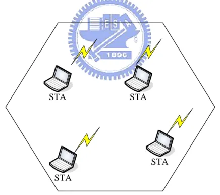
(13) Chapter 2 Medium Access Control of Wireless Local Area Network The IEEE 802.11 standard includes the MAC and PHY, this thesis focuses on the core of the MAC. This chapter first introduces the architecture of the WLAN, which includes the components, topologies and some nomenclature. The IEEE 802.11 MAC includes lots of control functions, such as medium access control functions, power saving function and other management functions. While in this chapter, only the relevant medium access control functions are detailed. The original medium access control functions in the IEEE 802.11 are first depicted, which include DCF, PCF. The enhanced medium access control mechanisms in the IEEE 802.11e, which include the EDCF and HCF, are addressed after the IEEE 802.11.. 2.1 Architecture of Wireless Local Area Network Before the detailed MAC description, the overview to the WLAN architecture will be described briefly. From the network topology perspective, it could be separated as independent basic service set and infrastructure basic service set. This section starts from the basic components, the network topologies and then the whole architecture. 2.1.1 Components The WLAN includes three entities from the generic perspective: the station (STA), the access point (AP) and the wireless medium (WM). The STA is the most basic component of the WLAN. A STA could be any device that maintains the defined 5.

(14) functionality of the IEEE 802.11 standard. The AP acts as a bridge between the wireless and wired network, it aggregates all the access to and from the wired or wireless network for the STAs. An AP is usually composed of a radio, a wired network interface (e.g. 802.3), and a bridging software that conforms to the 802.11d bridging standard. The WM is the medium used to implement the delivery of the protocol data units (PDU) between the PHY entities of the WLAN. A collection of STAs that communicate with each other is said to construct a basic service set (BSS). The BSS is the basic building block of the WLAN as shown in Figure 2-1. It is useful to view the hexagon as the coverage area (the conceptual not the practical coverage) and the STAs within the area can communicate to each other. If a STA moves out of the coverage, it can not communicate with the other member in the BSS.. STA. STA. STA STA. Figure 2-1, Basic Service Set. 6.

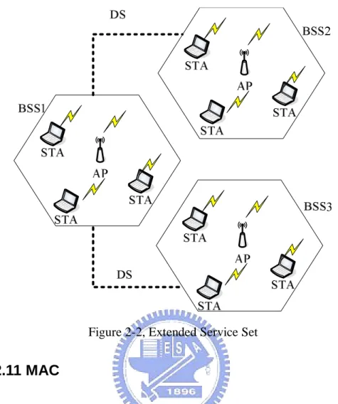
(15) 2.1.2 Topologies The most basic WLAN topology is a set of STAs, which have recognized each other and connected by the WM in the peer-to-peer fashion. When all the STAs in the BSS are mobile STAs and there is no connection to the wired network, this form of network topology is referred to independent basic service set (Id-BSS) or an ad-hoc network. Id-BSS typically is a short-lived network that is created for specific purpose. When a BSS includes an AP, this BSS is called infrastructure basic service set (If-BSS). The AP provides the relay function for the BSS. The STAs within the If-BSS communicate with the AP and there is no direct communication between the STAs. The If-BSS is desirable for several reasons compared to the Id-BSS. The presence of an AP enables the contention-free operation mode (the difference between the contention and contention-free control will be addressed in the next sub-section). The data communication between the STAs can be controlled by the higher priority AP under the contention-free mode, that is, the reasonable guarantees of the QoS are feasible. Besides, the AP enables the significant power-save mode that expands the battery life of the portable STAs. The AP buffers the data belong to those STAs and delivers to those STAs at a convenient time. The STAs awake to receive the data once in a while and result in the longer battery life. The AP may also provide connection to the distribution system (DS) and form the extended service set (ESS) as shown in Figure 2-2. The DS is the backbone network of the WLAN and may be constructed by either the wired or wireless network. In the ESS mode, the APs act as entries, they forward the traffic from one BSS to another or communicate with other networks via the DS. The benefic of the ESS is that it can facilitate the STA’s movement, that is, one can move from one BSS to another without losing the connection. 7.

(16) Figure 2-2, Extended Service Set. 2.2 802.11 MAC There are two medium access mechanisms provided by the IEEE 802.11 standard: the Distributed Coordination Function (DCF) and the optional Point Coordination Function (PCF). This section first details the mandatory DCF and then the optional PCF. 2.2.1 Distributed Coordination Function The fundamental medium access mechanism of the IEEE 802.11 is the DCF, which is based on Carrier Sense Multiple Access with Collision Avoidance (CSMA/CA) and can provide the fair chance of accessing the medium. The CSMA sometimes is called “listen-before-talk” scheme, the STA senses the medium before data delivery. Before the whole control function and the mechanism flow of the DCF, there are three issues should be addressed first: the reliable data delivery, the 8.

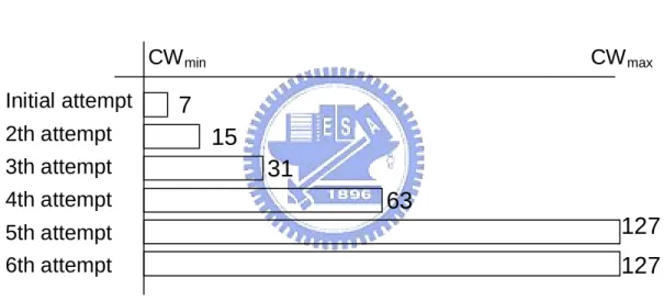
(17) inter-frame space and the binary exponential backoff. The WLAN technology operates on the unlicensed industrial, scientific and medical (ISM) band (802.11b/g on 2.4 GHz and 802.11a on 5GHz). To provide the reliable data delivery on the noisy and interference ISM band, the acknowledgement frame (ACK) is necessary mostly. The source STA expects the ACK frame after the transmission to the destination, and the STA will try to retransmit if it does not get the ACK frame. The inter-frame space (IFS) is the time interval between frames. There are four kinds of IFS defined to provide multiple priorities for medium access. The four IFSs from the shortest to the longest are short IFS (SIFS), PCF IFS (PIFS), DCF IFS (DIFS) and extended IFS (EIFS). The SIFS is the minimum time interval between any two frames. Using the smallest gap within the frame exchange can prevent other STAs from attempting to use the medium, thus giving the priority to the completion of the frame exchange in progress. The PIFS is used by the AP to gain the access over the medium. The value of the PIFS is one SIFS plus one slot time1. The DIFS is used for a STA wishes to start a transmission, which is the SIFS plus two slot times. The EIFS is much larger than other kinds of IFS and is the interval required between a STA’s attempts on the retransmission of a failed packet. A collision occurs when multiple STAs simultaneously transmit on the shared medium. The DCF protocol mandates the STA attempts to transmit must execute a backoff procedure to reduce the probability of collision and provide fair access opportunities for other aspiring STAs. The binary exponential backoff procedure works as follows: A STA wishes to transmit sets the backoff timer as Equation 1. The 1. The value of the xIFS and a slot time (aslottime) depend on the physical configuration (802.11a, b,. g). 9.

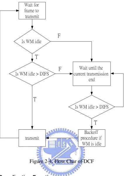
(18) value of the timer is a uniformly distributed random number ranged from zero to the Contention Window (CW). The timer decreases when the medium is free and is frozen when the medium becomes busy. After the backoff timer expires, the STA has the opportunity to transmit. The CW will double for each successive attempt to transmit the same packet as shown in Figure 2-3. Once the CW reaches the maximum value (CWmax), it shall stay at the value until it is reset. On the other hand, for a successful transmission, the CW will be reset to CWmin.. backoff = Random[0, CW ] × aslottime CWmin ≤ CW ≤ CWmax. (1). CW min Initial attempt 2th attempt 3th attempt. CW max. 7 15 31. 4th attempt. 63. 5th attempt. 127. 6th attempt. 127 Figure 2-3, Binary Exponential Increase of CW. Figure 2-4 is the flow char of the STA under DCF access operation. The rule of the DCF is that a STA desiring to transmit senses the medium, if the medium is idle for a DIFS, the STA commences transmitting data. Otherwise, the STA defers the transmission until the end of other STA’s transmission, and then it waits for another DIFS and performs the aforementioned backoff process.. 10.

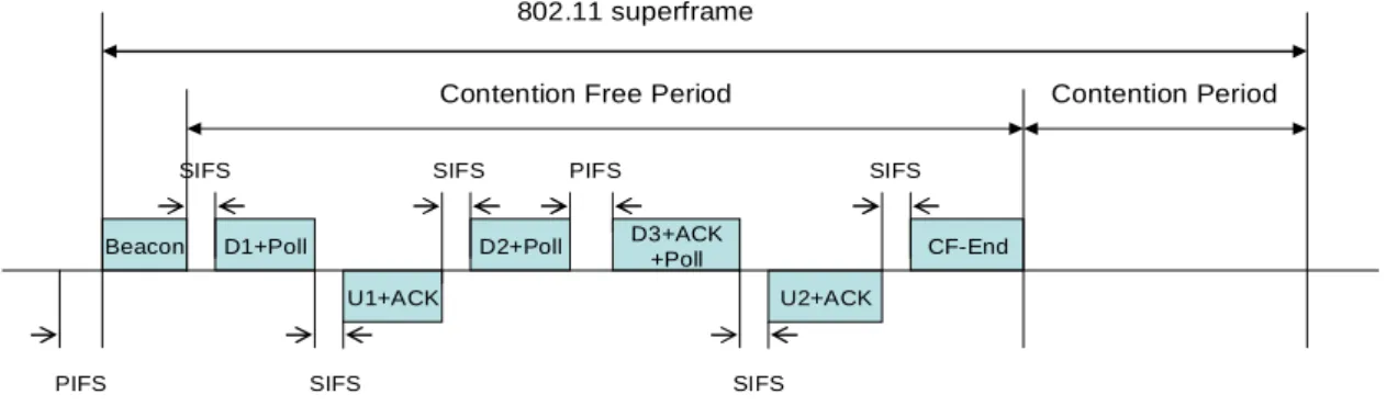
(19) Figure 2-4, Flow Char of DCF 2.2.2 Point Coordination Function Apart from the DCF, the Point Coordination Function (PCF) provides contention-free access mechanism to let STAs have priority access to the medium and to implement the time-bounded services. When the PCF is implemented, the time is always divided into two alternated periods (contention-free period and contention period, CFP and CP) and forms a periodic superframe structure. Under this access mode, the medium control is belonged to an access point (AP), which is referred to a point coordinator. The AP polls the STA having the contention-free traffic and then routes the data to the destination. During the CFP, the AP maintains a polling list which records the eligible CF-Pollable STAs and polls these STAs one by one. To become the CF-Pollable STA, 11.

(20) a STA should request to AP early. Upon receiving a poll frame, the STA transmits its data after a SIFS period. If the AP receives no response from the polled STA, the AP will poll the next STA after a PIFS. In short, there is no idle period larger than a PIFS value. If the AP has completed the polling of all STA recorded on the polling list, it can end the CFP by the CF-End frame and release the access to other contented STA. To make the bandwidth more efficient, the piggyback scheme is utilized. The concept of the piggyback is that the control frame (e.g. ACK) and the data frame (e.g. Data) are combined whenever applicable, such as Data+CF-ACK, CF-Poll+CF-ACK and Data+CF-Poll+CF-ACK. A superframe starts from the beacon frame broadcasted by the AP, and then the PCF and DCF operate on the CFP and the CP respectively. Figure 2-5 depicts the superframe structure and the mentioned PCF operation on the CFP. The beacon frame is the management frame that includes the synchronization and other protocol related parameters. One important parameter is the target beacon transition time (TBTT) which announces when the next beacon frame will arrive, so the AP can ideally2 generate the periodic superframe.. 802.11 superframe Contention Free Period SIFS. Beacon. SIFS. D1+Poll. D2+Poll. PIFS. SIFS D3+ACK +Poll. U1+ACK. PIFS. Contention Period. CF-End U2+ACK. SIFS. SIFS. Figure 2-5, PCF Operation on CFP of Superframe 2. In practice, the superframe is not absolute periodic due to the contention. Section 2.3.1 will detail this. issue. 12.

(21) 2.3 802.11e MAC There are some limitations for the traditional 802.11 MAC to maintain the QoS requirements, such as the required bandwidth and bounded delay. To support the QoS, the enhanced control functions which include the Enhanced Distributed Coordination Function (EDCF) and the Hybrid Coordination Function (HCF) are promoted by the IEEE 802.11 Task Group E (TGe). The EDCF is a contention-based channel access extended from the DCF, and the HCF combines both the contention-based channel access and the polling-based channel access, that is, EDCF could be viewed as a part of the HCF. The limitations of the original 802.11 MAC and both the enhanced control functions will be described in this section. 2.3.1 Enhanced Distributed Coordination Function The DCF does not support any QoS assurance. Basically, the DCF provides the fair channel access probability without the concept of service differentiation to all STAs, that is, all STAs contend the bandwidth with the same priority. It is not a desirable feature since the time-bounded services, such as the VoIP and videoconference, have the specified bandwidth and low delay requirements. Several studies have proved the poor performance of the DCF for supporting the real-time services [20, 21]. The EDCF is an extension of the DCF and it utilizes the similar CSMA/CA operation concept. To provide the prioritized QoS, the Access Categories (ACs) and multiple independent backoff entities are introduced. Eight different priority traffics are mapped into four Access Categories (ACs), each AC (queue) performs backoff individually and has its own parameter set, which includes the Arbitration IFS (AIFS[AC]), CWmin[AC], CWmax[AC], and Transmission Opportunity (TXOP[AC]) 13.

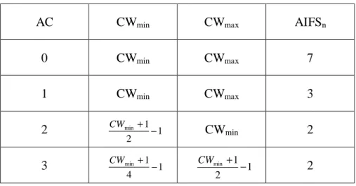
(22) where the AIFS[AC], CWmin[AC] and CWmax[AC] replace the DIFS, CWmin, and CWmax of the DCF respectively and the TXOP is the maximum duration that a station can transmit. Table 2-1 and Table 2-2 are the traffic priority mapping and the typical EDCF parameters respectively. In Table 2-2, the AIFSn is used to calculate the AIFS (AIFS[AC] = SIFS + AIFSn×aSlotTime). A low-priority AC has larger values of AIFSn, CWmin, and CWmax than a high-priority AC. Hence, the high-priority traffic is likely to access the medium easily than the low- priority traffic. Table 2-1, Priority to Access Category Mapping Priority. Access. Destination. 1. 0. Best Effort. 2. 0. Best Effort. 0. 0. Best Effort. 3. 1. Video Probe. 4. 2. Video. 5. 2. Video. 6. 3. Voice. 7. 3. Voice. Table 2-2, Typical EDCF Parameter AC. CWmin. CWmax. AIFSn. 0. CWmin. CWmax. 7. 1. CWmin. CWmax. 3. 2. CWmin + 1 −1 2. CWmin. 2. 3. CW min + 1 −1 4. CWmin + 1 −1 2. 14. 2.

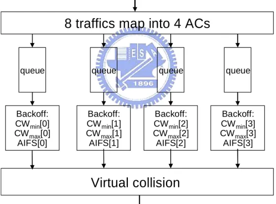
(23) Figure 2-6 is the reference model of the 802.11e STA, the four individual backoff entities perform virtual collision within a STA. As the collision occurs on the medium, it is possible that the backoff timers of the different queues are expired at the same time. The highest priority traffic frame are transmitted, and the other traffic queues perform the collision operation as they collide with other STA when more than one timer expiration within the STA. It should be noted that the highest priority traffic may also collide with other STA on the medium. By the virtual collision mechanism and the AC parameter set, the applications of each STA are served differentially.. 8 traffics map into 4 ACs. queue. queue. queue. queue. Backoff: CW min[0] CW max[0] AIFS[0]. Backoff: CW min[1] CW max[1] AIFS[1]. Backoff: CW min[2] CW max[2] AIFS[2]. Backoff: CW min[3] CW max[3] AIFS[3]. Virtual collision Figure 2-6, Reference Model of 802.11e STA. 15.

(24) 2.3.2 Hybrid Coordination Function The PCF is designed to support the time-bounded service, while it has three main limitations. First, the unpredictable beacon frame delay due to the alternation of the CFP and CP. The STAs are allowed to start their transmission even if the current packet can not finish before the upcoming TBTT. The delay beacon frame leads to extra delay for the time-bounded services. Second, it is no assurance of the transmission time for each polled STA. This makes the AP hard to provide guaranteed performance during the CFP. Third, the communication within an If-BSS should go through the AP and results in bandwidth inefficiency. The HCF is based on the polling mechanism as defined in PCF and a few improved and extended control mechanisms. First, a STA is not allowed to deliver if the transmission can not be completed before the upcoming TBBT, which solves the beacon frame delay problem. Second, a TXOP is used to limit the transmission time for the polled STA. Third, the direct link protocol (DLP) defines how to communicate within an If-BSS. These improvements can help the AP make the bandwidth allocation more precise and reduce the waste of the bandwidth. Furthermore, the auxiliary of negotiated traffic specification (TSPEC) and the non-existing boundary of the CFP and CP promote the capability of QoS supporting. To setup a specific traffic service, a STA must send a request frame containing the TSPEC to the AP. The TSPEC describes the required QoS parameters such as mean data rate, delay bound, and etc. Based on the parameterized requirement, the AP grants or rejects the service. If the service is admitted, the AP is responsible for maintaining the QoS demands. Besides, different from the strictly separate relation of the 802.11 MAC (PCF and DCF), the HCF combines both advantages to adaptively manager the bandwidth. When HCF is implemented, a Hybrid Coordinator (HC) 16.

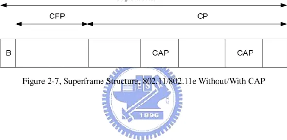
(25) resides in the AP takes the responsibility of managing the wireless medium. The most differences are that in HCF, the AP has the highest priority so as to poll STAs to maintain the QoS demands even during the CP. The period that the AP polls stations in the CP is called Controlled Access Period (CAP), as shown in Figure 2-7. The pre-information of the auxiliary TSPEC and the flexible drive of the polling-based channel access can make the bandwidth assignment more precise and efficient and further guarantee the required QoS.. Figure 2-7, Superframe Structure, 802.11/802.11e Without/With CAP. 17.

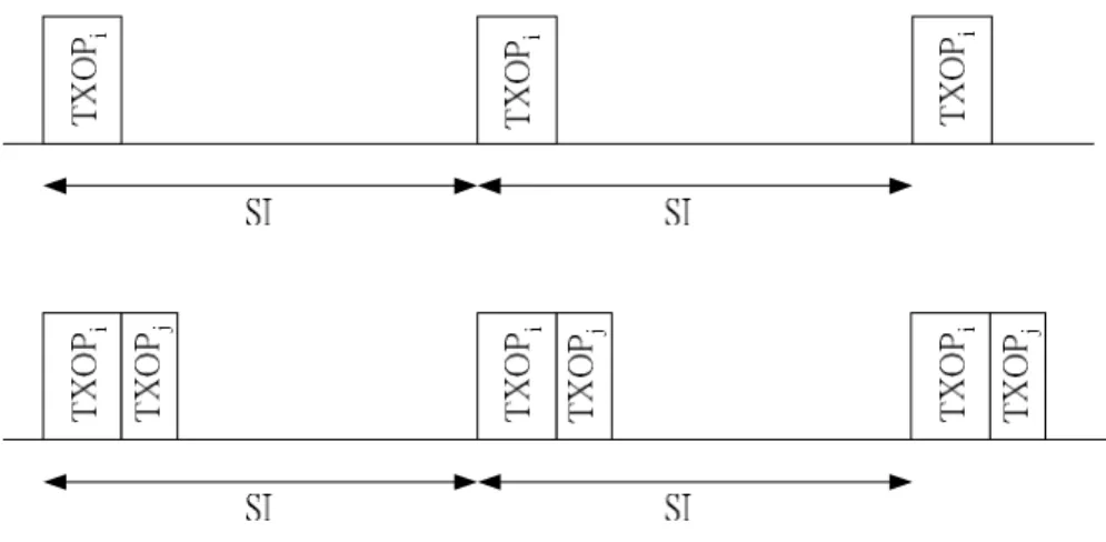
(26) Chapter 3 Scheduling Algorithms in WLAN Chapter 2 has introduced the enhanced medium access control function, and furthermore this chapter describes the scheduling control algorithm applied to the polling-based channel access of the HCF. The simple scheduling control algorithm provided by the vendors of TGe will be addressed first and followed by the proposed timer-based scheduling control algorithm.. 3.1 Simple Scheduling Algorithm The simple scheduling algorithm is based on fixed order polling mechanism. The AP calculates a fixed Service Interval (SI) and TXOP for each station based on Mean Data Rate (ρ), Nominal MAC Service Data Unit (MSDU) Size (L), and Maximum Service Interval (MSI) or Delay Bound (DB) of the TSPEC. Figure 3-1 shows how the simple algorithm to allocate the bandwidth, the unmarked (blank) portion in the SI is reserved (utilized) for the contention-based channel access. When a new stream participates, the AP determines the SI, and then the AP reserves (allocates) the TXOP for each service. The SI and TXOP are calculated as follows:. Figure 3-1, Bandwidth Allocation of Simple Algorithm 18.

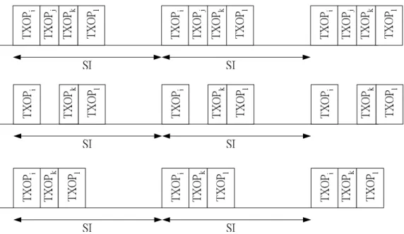
(27) For the SI, the AP first calculates the minimum of all MSIs (or DB) as a value m. Then, the AP determines the SI that is the sub-interval of the beacon interval value and is lower than the value x as shown in Equation 2, where BI represents the beacon interval and the m is an integer. The SI will be re-calculated when a new traffic stream is admitted and the MSI (or DB) of the incoming service is less than the current SI. For TXOP, as shown in Equation 3, the AP first calculates the number of the MSDUs (N) that arrives at the Mean Data Rate during the SI. After that, from Equation 4, the AP calculates the TXOP as the maximum of the time to transmit frames calculated in Equation 3 and the time required to transmit the maximum size of MSDU (M, 2304 bytes) at transmission rate of user i, Ri, and then plus the overheads (O). The overheads include the PHY and MAC header and inter-frame space. SI =. BI ≤ x = min {MSI i ( DBi )} i m. (2).  SI × ρ i  Ni =    Li . (3).  N × Li M  TXOPi = max  i ,  + O R Ri  i . (4). Next, consider the bandwidth reallocation after the dropped stream. If a stream is dropped, the AP may resume the available time and leave it for contention or move the following TXOPs to prevent the intermittent alternation of the polling-based and contention-based channel accesses. An example depicted the two schemes is shown in Figure 3-2, when the traffic j is removed.. 19.

(28) Figure 3-2, Reallocation of TXOPs. 3.2 Proposed Timer-Based Scheduling Algorithm The proposed timer-based scheduling algorithm is based on the concept of the Earliest Deadline First (EDF) and utilizes the mean inter-arrival time of the consecutive frames and the delay bound to effectively control the required transmission rate and delay budget for achieving QoS requirements. In the proposal, the AP sets two timers for each direction of a bi-directional service, and then determines which STA has the lowest timer. The setups of the timers are as follows: The downlink timer is used to calculate the deadline of a downlink frame. As calculated in Equation 5, the deadline of the frame from the network is the delay bound (DB) minus both the frame age (Age, the time that the frame has stayed in the MAC layer) and the required time to finish the transmission of the frame (Tt). Td = DB − Age − Tt. (5). 20.

(29) The uplink timer is used to estimate the uplink deadline of the next frame. Figure 3-3 shows how to set the uplink timer. A STA that intends to join the If-BSS will send requests to the AP. If the AP accepts the station, the uplink deadline is set based on Equation 6, which is the estimated time of the first frame plus the delay bound and minus the time to exchange frame. After polling the STA, the new uplink timer will be updated based on Equation 7, which is the remaining value of the timer (Told) plus the mean frame inter-arrival time (Tint). Tu = Te + DB − To. (6). where Te represents the estimated time of the first frame, and To represents the time to exchange frames. Tu , new = Tu ,old + Tint. ∀ Polled STA. = Tu ,old. ∀ Other STAs. (7). Figure 3-3, Uplink Timer Setup Relationship. 21.

(30) Figure 3-4 is the flow of the timer-based scheduling control algorithm. To facilitate the understanding, the margin timer (Tm, calculated as Equation 8) and the threshold (Tthr) are introduced. The margin timer represents the margin of the most urgent packet and the threshold is used to separate the contention-based and polling-based channel accesses. The AP compares the margin timer with the threshold to determine whether the polling-based access function should be commenced. If the margin timer is less than the threshold, the AP will start the polling-based channel access (CFP or CAP) otherwise the bandwidth will be released for the contention-based channel access. Tm = min {min{Ti ,d , Ti ,u }}. (8). i. Tm = min{min{Ti,d , Ti,u }} i. Tm > Tthr. Figure 3-4, Flow Char of Proposed Algorithm. 22.

(31) The threshold has a big impact on the performances. The larger threshold biases against the EDCF since the resource is always occupied by the polling-based channel access, which results in the lower throughput of the non real-time service. On the contrary, the smaller threshold may cause the serious delay of the real-time services. Hence, there exists a tradeoff between the delay of the real-time services and the throughput of non real-time services. Based on the flow char of the algorithm, the packet will be transmitted after it becomes the most urgent packet and the timer is less than the threshold. The relation of the delay of the packet (D(n)) and the margin timer is shown in Figure 3-5 and expressed as Equation 9, where n represents the frame sequence. Equation 9 could be written as Equation 10 from the statistics concept, the D in Equation 10 represents the average delay. To provide service differentiation and relative delay fairness, Equation 10 is modified as Equation 11. In this case, compared to the most urgent service, the other services will always tolerate a delay gap and the value of this gap is the difference of delay bound. For a given objective (expected) delay (Dobj), Equation 11 is written as Equation 12. The meaning of Equation 12 is that to achieve the objective delay, the threshold should be at least larger than a specific value.. Generally, the. delay increases with the loading of the real-time service. It is impracticable to desire an extreme delay for heavy loading. This causes great degradation in the throughput without improving the delay. To simplify, a threshold mapping table is suggested, the detailed setup is described in the next chapter. D (n) ≅ DB − Tm (n) ≥ DB − Tthr. (9). D = E[ D (n)] ≥ DB − Tthr ⇒ Tthr ≥ DB − D. (10). Tthr ≥ min{DBi } − D. (11). Tthr ≥ min {DBi } − Dobj. (12). i. i. 23.

(32) Figure 3-5, Relation of Delay and Minimum Timer. 3.3 Analysis of Algorithms’ Concept The last two sub-sections have described how to implement the simple and the proposed timer-based scheduling control algorithms. Before immediate simulation and comparison, this sub-section first analyzes the designed concept by intuition. The simple algorithm serves each STA once per service interval. The AP regards each stream as constant bit rate (CBR) service and treats them equally without considering the different QoS requirements, that is, the AP reserves the bandwidth for the service if it was admitted. It is inefficient in some scenarios. First, lots of real-time applications are variable bit rate (VBR) service, so the characteristic of the burst data should be emphasized. For example, if the generated data is small and the AP still polls the STA, this will cause the bandwidth inefficiency since the station has no data to transmit. Second, the fixed SI for each service results in the same delay for each service, while this is impracticable since some services have looser requirements. 24.

(33) especially under the mixed traffic scenario. In short, the performance degrades under the insidiously simple scheduler design. Compared to the simple algorithm, the timer-based algorithm is more flexible. The standard endowed the AP with the highest priority to start the CAP, but the powerful feature is seldom considered in the simple algorithm. On the other hand, the CAP is utilized in the timer-based algorithm as needed. The urgent traffic is served earliest and the service differentiation is also considered. The timer-based algorithm does not emphasize the absolute fairness in delay since the delay requirement is different. By utilizing the influential CAP properly and sacrificing the looser QoS requirement service without violating the demands can make the bandwidth utilization more efficient and adaptable.. 25.

(34) Chapter 4 Simulation Results In this chapter, the comparisons of the mentioned access mechanisms which include the contention-based EDCF, the simple and the timer-based scheduling control algorithms are explored. The simulation model which includes the environment setting, the assumptions and the performance metrics will be addressed first to facilitate the understanding of the simulation. Then the complete simulations and mutual comparisons are depicted in section 4.2.. 4.1 Simulation Model The simulation is modeled as an infrastructure mode where one AP exchanges sequences with multiple STAs and each STA has only traffic stream. Two real-time services (bi-direction) and a simple non real-time service (only used in the contention phase) are considered in this study. The voice services are modeled as a constant bit rate of 64 Kbps (160 bytes per 20 ms frame). For video services, with 25 fps (frame-per-second), the frame length follows a truncated lognormal distribution with the mean and standard deviation of 1300 bytes and 260 bytes respectively. The ITU recommends the acceptable one way delay of the voice service is at most 150 ms [22]. So the delay bound of the voice is set to 25 ms since the Internet delay and coding delay are 100 and 25 ms respectively [23]. The delay bound of the video service is not as tight as the voice service and will be set at 50 ms. The non real-time data traffic is modeled as exponentially distributed inter-arrival time (25ms) with fixed frame size (500 bytes), which results in 160 kbps.. The source parameters and system. parameters are summarized in the Tables 4-1 and 4-2 respectively.. 26.

(35) Table 4-1, Traffic Parameters Service. CBR Voice. VBR Video. Max bit rate. 64 Kbps. 600 Kbps. Mean bit rate. 64 Kbps. 260 Kbps. Min bit rate. 64 Kbps. 100 Kbps. Nominal MSDU size. 160 bytes. 1300 bytes. Delay bound. 25 ms. 50 ms. Table 4-2, System Parameters RTP/UDP/IP header. 12/8/20 byte. PHY/MAC header. 24/36 byte. PHY header rate. 1 Mbps. MPDU rate. 11 Mbps. SIFS. 10 us. PIFS. 30 us. Aslottime. 20 us. Voice(CWmin,CWmax). (7, 15). Video(CWmin,CWmax). (15, 31). Data (CWmin,CWmax). (31,255). Voice/Video AIFS. 50/50 us. Data AIFS. 70 us. The performance metrics considered in the simulation are defined as follows: • Delay: The time between the packet arrival (entering the MAC) and the successful reception of the packet, i.e. it includes queuing and transmission delay. • Packet loss rate: The fraction of discarded packet caused by violating the delay bound. • Capacity: The number of the stations (at a fixed transmission rate) that the system can support. • Data throughput: In the study, the data throughput is the sum of downlink and uplink throughput of the non real-time data traffic.. 27.

(36) Before discussing the simulation results, several assumptions are also made for this study: • The first-in-first-out (FIFO) will be considered for the contention (EDCF) implementation. • The transmission channel is error free. A packet loss happens only if the delay bound expires and the packet will be discarded without transmission. • To simplify the SI allocation, the beacon frame is ignored. • For the simple algorithm, if the transmission of the real-time service exceeds the SI, the next SI will start immediately without releasing the resource for the contention-based channel access.. 4.2 Simulation Results Based on the model mentioned as the last sub-section, the full simulations are made to measure the performance, which include: (1) the comparison of the contention-based and polling-based channel access mechanisms, (2) the comparison of the “prototype” scheduling algorithms, (3) the comparison of the practicable scheduling algorithms, and (4) the influences of the scheduling algorithms’ parameter. The “prototype” represents that there is no contention-based channel access in the bandwidth utilization3. For simple algorithm, the AP serves those STAs one by one without considering the SI. For proposed algorithm, the AP always serves the STA with the minimum timer.. 3. The prototype is not practical scenario since the standard defines the minimum time of the. contention-based channel access, but it can assist in figuring out the original feature from the simulation perspective. 28.

(37) 4.2.1 Contention-Based and Polling-Based Channel Access Mechanisms Recall that there are two extended medium access function provided by the IEEE 802.11 TGe, the EDCF and the HCF. The EDCF can provide prioritized service, but its performance degrades severely at the heavy loading in the If-BSS [15-17]. Hence, the pure contention-based channel access (EDCF only) and the polling-based channel access based on the prototype simple scheduling algorithm are first evaluated to emphasize the urgent necessary of the polling-based channel access. Figure 4-1 and 4-2 show the average delay and packet loss rate of both the downlink and uplink streams under the increasing voice service scenario. The downlink phase represents the delivery direction from the AP to STA and the uplink one is the direction from the STA to AP. As expected, the delay increases with the increment of service no matter the contention-based EDCF or the prototype simple algorithm. Besides, the downlink transmission limits the EDCF capability. When the number of service is below a value, the EDCF performs better than the prototype simple algorithm. The delay of the EDCF maintains nearly at the fixed value when the service number is less than ten, and the delay of the prototype simple algorithm increases linearly under no packet loss condition. On the other hand, when the service number exceeds some value, the asymmetric transmission causes serious problem. The AP works as a normal STA to contend the medium but it buffers all the STAs’ downlink traffics, that is, each downlink flow shares only a fraction of the transmission opportunity contended by the AP. Figure 4-2 shows the situation, the capacity of the downlink and uplink are thirteen and seventeen respectively which are far smaller than the prototype simple algorithm (twenty-seven) under the 2% packet loss rate constraint. In short, the EDCF can perform well under the light loading, while the prototype simple algorithm can support more services than the EDCF. 29.

(38) Figure 4-1, Delay, EDCF vs. Prototype Simple Algorithm. Figure 4-2, Packet Loss Rate, EDCF vs. Prototype Simple Algorithm. 30.

(39) 4.2.2 Prototype Comparison of Simple and Proposed Algorithm It is found that the prototype simple algorithm can support more users than the EDCF. This sub-section further compares the proposed timer-based algorithm to the simple algorithm from the prototype perspective. To point out the influence caused by the simple and timer-based algorithms respectively, the simulation scenario is to fix the video service number and gradually increase the voice number. Figure 4-3 and 4-4 are the average delay and packet loss rate under a fixed of six video service case. The simple algorithm considers the absolute fairness in the delay control, but the timer-based algorithm provides service differentiation. As shown in Figure 4-3, the voice’s and video’s delay performances are similar, since the simple algorithm has the same treatment for all applications. The slight difference is due to the transmission time. The suddenly severe increment in the delay implies that the system can not support more service due to the packet loss (Figure 4-4). On the other hand, the timer-based algorithm controls the delay based on the delay bound requirements. The video’s delay requirement is not as strict as voice, it can tolerate more delay. Hence, by sacrificing the video’s delay without violating the requirement, the timer-based algorithm can support more voice services. In other words, if the scheduler control can not differentiate different services, one service could become the bottleneck for the system performance. With 2% packet loss rate constrain, the capacity of the mixed traffic is depicted in Figure 4-5, in which the proposal algorithm provides more capacity than the simple algorithm. To quantify the loading, assume that the loading is 1 when the capacity of voice and video are twenty-seven and sixteen respectively. The loading is calculated as Equation 13. The maximum loading of simple (timer-based) algorithm ranges from 0.861 to 1 (0.988 to 1.037). Besides, the proposed algorithm has relatively more gain 31.

(40) when the video service occupies more proportion. Loading =. N voice N video + N max,voice N max,video. (13). where Nvocie (Nvideo) represents the number of voice (video) service and Nmax,vocie (Nmax,video) represents the maximum number of voice (video) service the system can support.. Figure 4-3, Average Delay, Prototype. 32.

(41) Figure 4-4, Packet Loss Rate, Prototype. Figure 4-5, Capacity (2% Packet Loss Constraint). 33.

(42) 4.2.3 Practical Comparison of Simple and Proposed Algorithm The prototype condition is an extreme case that minimizes the contention-based channel access. It is found that the proposed timer-based algorithm can achieve higher capacity than the simple algorithm under mixed traffic condition in the last sub-section. Here, the practical algorithms will be addressed to further evaluate the performance. To make the timer-based algorithm practicable, the aforementioned threshold or the objective delay should be determined first. Based on the quantitative loading of sub-section 4.2.2, the relation of the loading (Figure 4-5 in the section 4.2.2) and the most urgent service’s delay (queuing delay only, since the transmission delay has variance for different service) is shown in Figure 4-6. It is obvious that the delay increases with the increasing loading and it is likely exponential increment. The threshold mapping attribute shown in Table 4-3 is based on the relation in Figure 4-6 and the setup steps are as follows: first, the loading is divided into several regions, and the maximum queuing delay for each region is taken out. Then the threshold is determined based on the minimum delay bound and the rough consideration of the transmission time (delay)4. Now, if there are ten voice and six video users, the loading will be 0.745, so the threshold will be set to 19.5. The infinite in Table 4-1 represents a large value, which prevents the contention. In practice, the AP should release resource for contention, which involves the resource reservation and is beyond the scope of this discussion.. 4. To decorate the threshold value, the transmission delay may have slight variance in different region. 34.

(43) Figure 4-6, Loading vs. Queuing Delay Table 4-3, Threshold Attribute Loading. <0.6. <0.7. <0.8. <0.9. <0.95. ≥ 0.95. Maximum queuing delay (ms). 1.2. 2.5. 4.8. 6.5. 7.5. >7.5. Threshold (if DB_min=25ms). 23. 22. 19.5. 18. 17. ∞. Threshold (if DB_min=50ms). 48. 47. 44.5. 43. 42. ∞. To simplify the contention loading problem, the downlink and uplink non realtime data traffics are both fixed to fifteen no matter how the loading of real-time traffic. Figure 4-7 and 4-8 show the average delay and data throughput at a fixed six video services circumstance (SI is 15 ms for the practicable simple algorithm). Compared with the prototype simulation results, the timer-based algorithm similarly provides service differentiation and results in the larger non real-time data throughput. 35.

(44) instead of the higher capacity. For the delay control, the result is similar with the prototype one. The difference is that the delay is almost fixed no matter how the service varies in the simple algorithm. In other words, when the SI is settled, the delay of each service is also determined. For the data throughput, it almost decreases linearly with the increasing voice number in the simple algorithm. While the data throughput of the proposed algorithm is deeply influenced by the threshold attribute. It decreases monotonously except at the case that the threshold changes to another value. Beside, the data throughput of the timer-based algorithm is larger than the supporting of the simple algorithm. Recall the prototype timer-based algorithm can support more users under the mixed traffic consideration, it could be thought as that the capacity gain transforms into the non real-time data throughput gain.. Figure 4-7, Average Delay, Practicable. 36.

(45) Figure 4-8, Data Throughput. 4.2.4 Influence of Algorithms’ Parameters The characteristics and the comparisons of both algorithms have been addressed in the last two sub-sections. The simulations show the proposed timer-based algorithm outperforms the simple algorithm under the mixed traffic consideration. Nevertheless, there exists adjustable parameter in each algorithm itself, and which may affect the performance. This sub-section will depict the influence of the algorithms’ parameters, which include the threshold for the timer-based algorithm and the SI for the simple algorithm. The threshold in the proposed timer-based algorithm is a tradeoff factor for the delay of the real-time services and the data throughput of the non real-time services. Figure 4-9 and 4-10 show how the threshold influences the data throughput and delay under the eight voice and six video services scenario. Both the data throughput and the delay reduce with the increasing threshold and vise versa. The data throughput of 37.

(46) the timer-based algorithm will be possibly less than the simple algorithm if the threshold setup is too aggressive (large). For example, in Figure 4-9, the throughput of the proposed algorithm is roughly equal to the simple algorithm when the threshold is equal to twenty-five. In short, the data throughput can be improved by sacrificing the delay of the real-time service.. Figure 4-9, Threshold vs. Data Throughput. 38.

(47) Figure 4-10, Threshold vs. Delay The SI in the simple algorithm has the similar function as the threshold in the timer-based algorithm. Figure 4-11, 4-12 and 4-13 show the data throughput, delay and packet loss rate under eight voice and six video services scenario. The notation “Tthr (normal)” in the three figures represents the normal threshold value based on the threshold attribute table. From those figures, it is obvious that the smaller SI benefits the real-time services (delay and packet loss reduction, but data throughput degradation) and vice versa. It should be marked that the packet lost exceeds 2% when the SI is equal to 25 ms in Figure 4-13. The reason is the SI is too long for the service. To deserve to be mentioned, the admission control mechanism of the AP (beyond the discussion) will more easily reject the new coming traffic when the SI is smaller.. 39.

(48) Figure 4-11, Service Interval vs. Data Throughput. Figure 4-12, Service Interval vs. Delay. 40.

(49) Figure 4-13, Service Interval vs. Packet Loss Rate It is known how the parameter in each algorithm itself influences the performances. Here, the mutual comparisons of Figure 4-9 ~ 4-13 will further show the superiority of the proposed algorithm. Since the design concepts of both algorithms are different (the simple algorithm focuses on the absolute delay fairness but the proposed algorithm emphasizes the service differentiation), the data throughput is viewed as the measurement. First, the proposed algorithm can provide higher data throughput than the simple algorithm under the 2% packet loss rate constraint. Second, the proposed algorithm supports a saturation region which represents the maximum throughput the system can support. For example, the data throughput of the proposed algorithm in Figure 4-9 is fixed at the threshold ranged from ten to fifteen. For the simple algorithm, the data throughput can rise monotonously, but the performance of the packet loss will also degrade significantly. In short, the proposed algorithm can provide higher data throughput under the appropriate threshold setup and the equal packet loss consideration. 41.

(50) Chapter 5 Conclusions and Future Works. 5.1 Conclusions To ensure the QoS in WLAN, this thesis investigates the capability of the 802.11e WLAN medium access control functions. Besides the EDCF defined by the standard and the simple scheduling control algorithm provided by the vendors of the TGe are introduced, the timer-based scheduling control algorithm is proposed to provide enhanced control mechanisms for handling different delay budgets for different applications. Based on the complete simulations, we have the following observations and conclude that the proposed timer-based scheduling control algorithm outperforms the simple algorithm. • The EDCF is not suitable for the infrastructure mode operation since the contention-based mechanism has a bias against the AP (downlink phase) and will cause worse performance when the loading is heavy. • The simple scheduling control algorithm serves each service equally, which results in the absolute delay fairness and the poor bandwidth utilization under the mixed traffic consideration. • The proposed timer-based scheduling control algorithm provides service differentiation without violating the QoS requirement and improves the bandwidth utilization, which results in either the larger capacity or the higher non real-time data throughput compared to the simple algorithm. • Each algorithm itself has adjustable parameter and the parameter is the tradeoff factors that can determine the performance. The mutual comparison further indicates the superiority of the timer-based scheduling control algorithm.. 42.

(51) 5.2 Future Works This thesis focuses on the bandwidth allocation of the resource management to provide the QoS. But there are other mechanisms mentioned in chapter 1 should also be taken into account. The most immediate is the call admission control (CAC). The vendors of TGe do not only provide the simple algorithm, but also the respective CAC algorithm. Of course, the CAC provided by the TGe can be applied to the timer-based algorithm, but it seems too conservative since the timer-based algorithm outperforms the simple one. Hence, to integrate the proposed scheduling algorithm and the CAC is the first step in the future.. 43.

(52) References [1] IEEE Std. 802.11, “Wireless LAN Medium Access Control (MAC) and Physical Layer (PHY) Specifications”, 1999. [2] IEEE Std. 802.11b, “Wireless LAN Medium Access Control (MAC) and Physical Layer (PHY) specifications: Higher-Speed Physical Layer Extension in the 2.4 GHz Band”, 1999. [3] IEEE Std. 802.11a, “Wireless LAN Medium Access Control (MAC) and Physical Layer (PHY) specifications Amendment 1: High-speed Physical Layer in the 5 GHz Band”, 1999. [4] IEEE Std. 802.11g, “Wireless LAN Medium Access Control (MAC) and Physical Layer (PHY) specifications Amendment 4: Further Higher Data Rate Extension in the 2.4 GHz Band”, 2003. [5] G. Bianchi, “Performance Analysis of the IEEE 802.11 Distributed Coordination Function”, IEEE Journal, Selected Areas in Communication, vol. 18, no. 3, pp. 535-547, Mar. 2000. [6] Y. Xiao and J. Rosdahl, “Throughput and Delay Limits of IEEE 802.11”, IEEE Communication Letter, vol. 6, no. 8, pp.355-357, Aug. 2002. [7] J. Gozdecki, A. Jajszczyk and R. Stankiewicz, “Quality of Service Terminology in IP Networks”, IEEE Communication Magazine, vol. 41, no. 3, pp. 153-159, Mar. 2003. [8] L. C. Wolf, C. Griwodz and R. Steinmetz, “Multimedia Communication”, Proceedings of the IEEE, vol. 85, no. 12, pp. 1915-1933, Dec.1997. [9] IEEE Std. 802.11e/D3.0, “Wireless LAN Medium Access Control (MAC) and Physical Layer (PHY) Specifications: Medium Access Control (MAC) Enhancements for Quality of Service (QoS), May 2002. [10] W. Pattara-Atikom, P. Krishnamurthy and S. Banerjee, “Distributed Mechanisms for Quality of Service in Wireless LANs”, IEEE Wireless Communication, vol. 10, no. 3, pp. 26-34, June, 2003. [11] W. Liu, W. Lou, X. Chen and Y. Fang, “A QoS-enabled MAC Architecture for Prioritized Service in IEEE 802.11 WLANs”, IEEE GLOBECOM, vol.7, pp. 3802-3807, Dec. 2003. [12] A. Grilo and M. Nunes, “Performance Evaluation of IEEE 802.11E”, IEEE PIMRC, vol. 1, pp. 511-517, Sept. 2002. [13] H. Dajiang and C. Q. Shen, “Simulation Study of IEEE 802.11e EDCF”, IEEE VTC spring, vol. 1, pp. 22-25, April, 2003.. 44.

(53) [14] D. Chen, D. Gu and J. Zhang, “Supporting Real-time Traffic with QoS in IEEE 802.11e Based Home Networks”, IEEE CCNC, pp. 205-209, Jan. 2004. [15] Q. Ni, and T. Turletti, “QoS Support for IEEE 802.11 WLAN", Nova Science Publishers, New York, USA, 2004. [16] J. D. Prado, A. Soomro and S. Shankar, “Normative Text for Mandatory TSPEC Parameters and Informative text for a Simple Scheduler”, IEEE 802.11-02/705ar0, 2002. [17] A. Soomro, S. Shankar, J. D. Prado, Y. Ohtani, J. Kowalski, F. Simpson and I. L. W. Lih, “TGe Scheduler - Minimum Performance Requirements”, IEEE 802.11-02/709r0, 2002. [18] Y.L. Fan and C.Y. Huang, “Timer Based Scheduling Control Algorithm in WLAN for Real-Time Services”, IEEE ISCAS, May 2005. [19] Y.L. Fan and C.Y. Huang, “Real-Time Traffic Scheduling Algorithm in WLAN”, will be appeared in 4GMF, July 2005. [20] A. Kopsel and A. Wolisz, “Voice Transmission in an IEEE 802.11 WLAN Based Access Network”, Proc. WoWMoM, pp. 23-32, July 2001. [21] S. Choi, J. d, Prado, S. Shankar N and S. Mangold, “IEEE 802.11e Contention-Based Channel Access (EDCF) Performance Evaluation”, IEEE ICC, vol. 2, pp. 1151-1156, May 2003. [22] ITU Rec. G.114, “One-Way Transmission Time”, Feb. 1996. [23] T. J. Kostas, M. S. Borella, I. Sidhu,G. M. Schuster, J. Grabiec and J. Mahler, “Real-Time Voice over Packet-Switched networks”, IEEE Network, vol. 12, no. 1, pp. 18-27, Jan.-Feb. 1998.. 45.

(54)