應用於仿人眼視覺系統之智慧型深度偵測技術

國立交通大學

電機與控制工程學系

碩士論文

應用於仿人眼視覺系統之

智慧型深度偵測技術

Intelligent learning algorithm

for depth detection applied to a

humanoid vision system

研 究 生：張倍榕

A

指導教授：陳永平 教授

中 華 民 國 九 十 七 年 七 月

應用於仿人眼視覺系統之智慧型深度偵測技術

Intelligent learning algorithm for depth detection

applied to a humanoid vision system

研 究 生：張倍榕 Student：Pei-Jung Chang

指導教授：陳永平 Advisor：Yon-Ping Chen

國 立 交 通 大 學

電 機 與 控 制 工 程 學 系

碩 士 論 文

A Thesis

Submitted to Department of Electrical and Control Engineering College of Electrical and Computer Engineering

National Chiao Tung University in Partial Fulfillment of the Requirements

for the Degree of Master in

Electrical and Control engineering June 2008

Hsinchu, Taiwan, Republic of China

應用於仿人眼視覺系統之

智慧型深度偵測技術

學生: 張倍榕 指導教授: 陳永平 教授

國立交通大學電機與控制工程學系

摘 要

從兩台攝影機同時拍攝同景色的影像可以利用三角測量算出立

體座標點。但是如果要用這種方法求得立體座標需要對攝影機有一些

限制並且有一些參數是需要從實驗中獲得的。本論文提出用類神經網

路去訓練出不需要相機參數的深度偵測系統，訊練資料由不同變化的

目標點於兩張影像中的位置及其所對應的立體座標點構成。最後從誤

差百分比可以知道傳統的深度偵測演算法的誤差遠遠大於本論文所

提供的類神經網路深度偵測系統而且其準確度足以在立體視覺研究

中被應用。

Intelligent learning algorithm

for depth detection applied to a

humanoid vision system

Student：Pei-Jung Chang Advisor：Prof. Yon-Ping Chen

Department of Electrical and Control Engineering

National Chiao Tung University

ABSTRACT

Stereo–pair images obtained from two cameras can be utilized to compute world coordinate points by using triangulation. However, there are some restrictions from cameras and parameters need to be experimentally obtained, by applying this method. This thesis proposed that, for stereo vision applications which need to evaluate the actual depth, artificial neural networks be used to train the system such that the need for parameters of cameras are eliminated. The training set for our neural network consists of a variety of points in stereo-pair and their corresponding world coordinates. The percentage error obtained from the proposed architecture set-up is comparable with those obtained through traditional depth detection algorithm and that the system is accurate enough for most stereo vision applications.

Acknowledgment

兩年的研究生活，最感謝的是指導教授 陳永平老師的諄諄教導，老師總是 很有耐心的指導我所提出的疑問，讓我這兩年來在專業研究、學習態度上獲得很 多啟發。在此謹向老師致上最深的感謝之意。還有也感謝口試委員 楊谷洋老師 與 張浚林老師對於本論文所提出的指正與寶貴意見，使本論文能臻於完整。 此外，感謝可變結構控制實驗室的建峰、豐洲、桓展、世宏、子揚、士昌學 長們，在我的研究過程中提供許多的建議與經驗，讓我的研究更順利完成，同時 也感謝實驗室的同學琦佑、志榮以及學弟承育、新光、揚庭們曾經在研究中的協 助，讓我在實驗室的研究日子充滿歡樂。還有要特別感謝我的小舅舅及小舅媽， 讓我在新竹有個家，照顧我的生活，讓我在新竹求學日子無後顧之憂。最後要感 謝爸爸、媽媽以及關心我的親戚朋友們對我的支持及鼓勵，謝謝你們，我愛你們! 張倍榕 2008.8.28

Contents

Chinese Abstract...i

English Abstract...ii

Acknowledgement ... iii

Contents ... iv

Chinese Abstract...i

... iv

Index of Figures... vi

Chapter 1 Introduction... 1

1.1 Preliminary...1

1.2 Organization of the thesis ...2

Chapter 2 Intelligent learning algorithm ... 3

2.1 Introduction to ANNs...3

2.2 Back-Propagation Network...6

Chapter 3 Intelligent depth detection for a humanoid vision system

... 10

3.1 Humanoid Vision System Description...10

3.2 Depth Detection ...12

3.2.1 Traditional depth detection algorithm...12

3.2.2 ANN depth detection algorithm...18

Chapter 4 Experimental Results and Discussion... 21

4.1 Experimental Settings ...21

4.2 Experimental Results ...23

4.2.2 Flexibility of ANN Depth Detection Algorithm ...31

Chapter 5 ... 40

Conclusion ... 40

Index of Figures

Fig. 2.1 Basic element of ANNs ...3

Fig. 2.2 Multilayer feed-forward network ...5

Fig. 2.3 Back-propagation network ...7

Fig. 3.1 Humanoid vision system ... 11

Fig. 3.2 Relation of a world point projected onto an image plane...13

Fig. 3.3 Configuration of a HVS with binocular cameras ...14

Fig. 3.4 ANN model used for this thesis...19

Fig. 4.1 The board at Z=105cm captured form left camera ...22

Fig. 4.2 The board at Z=105cm captured form right camera ...22

Fig. 4.3 　L for different distance Z from 45 cm to 105 cm ...25

Fig. 4.4 　R for different distance Z from 45 cm to 105 cm ...25

Fig. 4.5 The same 12 points using to calculateΦ_L for Z=95cm ...26

Fig. 4.6 The same 12 points using to calculateΦ_R for Z=95cm...26

Fig. 4.7 Two adjacent points P1 and P2 in the center line of the training area for Z=135 ...26

Fig. 4.8 e_ave of two cameras placed in parallel with the same focal length ...28

Fig. 4.9 e_ave of two cameras with distinct focal length...29

Fig. 4.10 e_ave of two cameras with insignificant deflection between optic axes ...29

Fig. 4.12 ema in each depth simulated from the net...32

Fig. 4.13 ema of ten nets with five hidden neurons...33

Fig. 4.14 Each ema_Hn with one output neuron ...33

Fig. 4.15 Each ema_Hn with three output neurons...34

Fig. 4.21 The testing error of training data is obtained from Z=65, 115, 165cm...38 Fig. 4.22 The testing error of training data is obtained from Z=65, 95, 135, 165cm...39

Chapter 1

Introduction

1.1 Preliminary

The human brain can process subtle differences between the images that are observed at the left and right eyes to perceive a three-dimensional (3-D) in the space effortlessly. This ability of perceiving 3-D is called stereo vision. Recently, applications of stereo vision systems which have been proposed in telecommunication [1], geoscience [2], [3], navigation [4], [5], and robotics [6], [7], [8], [9], [10], [11], [12]. Although the 3-D reconstruction also can be achieved from a single image, a priori information is steel needed [13]. Thus, in order to simulate the ability of stereo vision that is similar to human eyes, a humanoid vision system (HVS) could be applied.

The HVS consists of two cameras, so that two images of the same scene can be taken at the same time by the right camera and the left camera from two different perspectives. The pair of these two images is called a stereo pair. The main problem in HVS is the perception of depth, because the depth information obtained from stereo vision is very useful for robot navigation in complex environments. Stereo vision consists of matching corresponding points in a stereo pair and estimating depth from their disparity which means the difference in positions of corresponding points. Usually in stereo vision systems, the depth is calculated from disparity by using the triangulation. The process of triangulation is needed to find the intersection of two known rays in space. This kind of classical technique needs careful calibration of the imaging system while calibration is an error sensitive process and it cannot always be performed online [13]. Therefore, there are some other approaches that calculating depth map without using camera parameter [12], [13]. In this thesis we have estimated

depth in a human visual system using neural networks. By using neural networks we have estimated depth without getting camera parameters and calibrating the imaging system.

1.2 Organization of the thesis

The rest of the thesis is organized as follows in chapter 2 we have introduced the intelligent learning algorithm. In chapter 3 we have represented the traditional depth detection algorithm and ANN depth detection algorithm respectively. In chapter 4 experimental results and discuss are provided. At last, chapter 5 represents the conclusions and future works.

Chapter 2

Intelligent learning algorithm

2.1 Introduction to ANNs

The human nervous system consists of a large amount of neurons, including somas, axons, dendrites and synapses. Each neuron is capable of receiving, processing, and passing electrochemical signals from one to another. To mimic the characteristics of the human nervous system, recently investigators have developed an intelligent algorithm, called artificial neural networks (ANNs), to construct intelligent machines capable of parallel computation. This thesis will apply ANNs to the depth detection in an eyeball system through learning.

.

.

.

.

.

.

y xi x3 x2 x1 bias wi w3 w2 w1

Σ

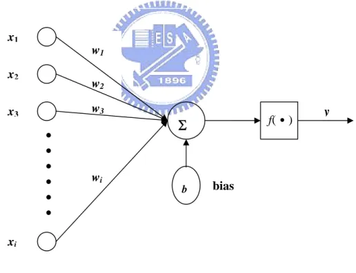
b f(․)

Fig. 2.1 Basic element of ANNs

ANNs can be divided into three layers which contain input layer, hidden layer, and output layer. The input layer receives signal form the outside world, which just includes input values without neuron. The neuron’s number of output layer is depending on the output number. Form the output layer, the response of the net can be

read. The neurons between input layer and output layer are belonging to hidden layer which does not exist necessarily. Here, each input is multiplied by a corresponding weight, analogous to synaptic strengths. The weighted inputs are summed to determine the activation level of the neuron. The connection strengths or the weights represent the knowledge in the system. Information processing takes place through the interaction among these units. The Basic element of ANNs, single layer net, is shown in Fig. 2.1 Basic element of ANNs which obeys the input-output relations

1 n i i i y f w x b = ⎛ = ⎜_⎝

∑

+ ⎟ (2.1-1) _⎠⎞

where wi is the weight at the input xi and b is a bias term. The activation function f(․)

has many types cover linear and nonlinear. Note that the commonly used activation function is

( )

- x

1 f x =

1+ e (2.1-2)

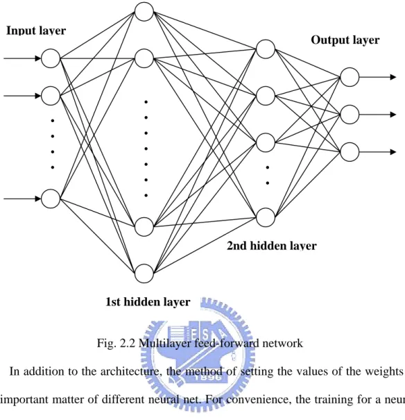
which is a sigmoid function. Base on the basic element, the commonest multilayer feed-forward net shown in Fig. 2.2 Multilayer feed-forward network, which contains input layer, output layer, and two hidden layers. Multilayer nets can solve more complicated problem than single layer nets, i.e. a multilayer nets is possible to solve some case that a single layer net cannot be trained to perform correctly at all. However, the training process of multilayer nets may be more difficult. The number of hidden layer and its neuron in the multilayer net are decided by complicated degree of the problem wait to solve.

Output layer Input layer 2nd hidden layer 1st hidden layer

.

.

.

.

.

.

.

.

.

.

.

.

.

Fig. 2.2 Multilayer feed-forward network

In addition to the architecture, the method of setting the values of the weights is an important matter of different neural net. For convenience, the training for a neural network mainly classified into supervised learning and unsupervised learning. Training of supervised learning is mapping a given set of inputs to a specified set of target outputs. The weights are then adjusted according to various learning algorithms. Another type, unsupervised learning, can self-organize neural nets group similar input vectors together without the used of training data to specify what a typical member of each group looks like or to which group each vector belongs. For unsupervised learning, a sequence of input vector is provided, but no target vectors are specified. The net modifies the weights so that the most similar input vectors are assigned to the same output unit. In addition, there are nets whose weights are fixed without iterative training process, called structure learning, which change the network structure to achieve reasonable responses. In this thesis, the neural network learns the behavior by

many input-output pairs, hence that is belongs to supervised learning.

2.2 Back-Propagation Network

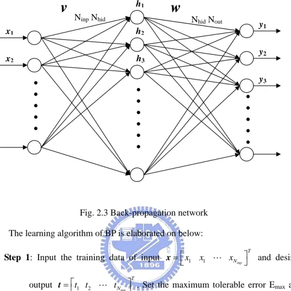
In supervise learning, the back propagation learning algorithm, is widely used in most application. The back propagation, BP, algorithm was proposed in 1986 by Rumelhart, Hinton and Williams, which is based on the gradient steepest descent method for updating the weights to minimize the total square error of the output. The training by BP mainly is applied to multilayer feed-forward network which involves three stages: the feed-forward of the input training pattern, the calculation and back-propagation of the associated error, and the adjustment of the weights. Fig. 2.3 Back-propagation network shows a back-propagation network contains input layer with Ninp neurons, one hidden layer with Nhid neurons, and output layer with Nout

neurons. In Fig. 2.3 Back-propagation network, _{1 1}

inp T N x x x x= ⎣⎡ " ⎤_⎦ , , and 1 2 _hid T N h h h h= ⎣⎡ " ⎤_⎦ 1 2 _out T N y y y

y= ⎣⎡ " ⎤_⎦ respectively represent the

input, hidden, and out note of the network. In addition, vij is the weight form the i-th

neuron in the input layer to j-th neuron in the hidden layer and wgh is the weight form

w

Nhid Nout y3 h3

v

Ninp Nhid x2 x1

.

.

.

.

.

.

.

.

.

.

.

.

.

.

.

.

y2 y1 h2 h1

Fig. 2.3 Back-propagation network The learning algorithm of BP is elaborated on below:

Step 1: Input the training data of input _{1 1}

inp

T N

x x x

x= ⎣⎡ " ⎤_⎦ and desired

output t=⎡t t_{1 2} " t ⎤T. Set the maximum tolerable error E and

inp

N

⎣ ⎦ max

leaning rate η which between 0.1 and 1.0 to reduce the computing time

.

Step 3: Calculate the output of the m-th neuron in hidden layer

d (2.1-3)

neuron and the output of the

i-th neuron in output layer

ut (2.1-4)

or increase the precision.

Step 2: Set the initial weight and bias value of the network at random

1 1 2 inp N m h k m k hi k h = f v x , m = , ,..., N = ⎛ ⎞ ⎜ ⎟ ⎜ ⎟ ⎝

∑

⎠

where fh(․)is the activation function of the

1 1 2 hid N n y mn m o q y = f w h , n = , ,..., N = ⎛ ⎞ ⎜ ⎟ ⎝

∑

⎠

where fy(․)is the activation function of the neuron.

Step 4: Calculate the error function between network output and desired output.

( )

(

)

1 1 1

2 n= n n 2 n= n y q= mn m

1 out 1 out hid

2 N N N 2 E w = d - y = ⎡⎢d − f _⎜⎛ w h ⎞_⎟⎤⎥ ⎢ ⎝ ⎠⎥ ⎣ ⎦

∑

∑

∑

(2.1-5)

Step ient steepest descent method, determining the correction of weights.

where yn is the network output and dn is the desired output.

5: According to grad

(

)

1 mn n n y mn m m mn m q mn n mn w y w = ∂ ∂ ∂ _{⎢ ⎥} hid N n y E E w η ∂ η ∂ ∂ η d - y ⎡f ′⎛ w h ⎞⎤h = hδ h Δ = − = − = ⎢ ⎜ ⎟⎥ ⎝

∑

⎠ (2.1-6) and ⎣ ⎦

(

)

1 1 1 1 n n y mn m mn h k m k k kmn k n= q= k= out inp out hid N n m km n km n m km N N N y h E E v v y h v d - y f w h w f v x x x η η η ηδ = ⎛ ∂ ∂ ⎞ ∂ ∂ Δ = − = − _{⎜ ⎟} ∂ _⎝∂ ∂ ∂ _⎠ ⎡ _′⎛ ⎞ ⎤ _′⎛ ⎞ = ⎢ ⎜ ⎟ ⎥ ⎜_⎜ ⎟_⎟ = ⎢ ⎝ ⎠ ⎥ ⎝ ⎠ ⎣ ⎦

∑

∑

∑

∑

(2.1-7) where

(

)

1 hid N mn n n y mn m q d - y f w h δ = ⎡ _′⎛ ⎞⎤ = _{⎢ ⎜ ⎟⎥} ⎢ ⎝ ⎠⎥ ⎣

∑

⎦

(

)

and d - y f w h w f v x δ = ⎡_⎢ ′⎛_⎜ ⎞_⎟ ⎤_⎥ ′⎛_⎜ ⎞_⎟ 1 1 1 n= q= k= inp out hid N N N kmn

∑

n n y

∑

mn m mn h ⎜

∑

k m k⎟.

Step 6: Propagate the correction backward to update the weights. 1 w n w n w ⎧ + = + Δ ⎪ ⎨ ⎢ ⎝ ⎠ ⎥ ⎝ ⎠ ⎣ ⎦

(

)

( )

(

1

) ( )

v n+ =v n + Δv ⎪⎩

7: Check whether the whole training data set have learned already.

Networks learn whole training data set once called a learning circle. If the network no

(2.1-8)

Step

to Step 8.

: Check whether the network converge. If E<E

Step 8 ining

, the BP algorithm was used to learn the input-output relationship for epth function.

max, terminate the tra

process; otherwise, begin another learning circle by going to Step 1.

BP learning algorithm can be used to model various complicated nonlinear functions. Recently years The BP learning algorithm is successfully applied to many domain applications, such as: pattern recognition, adaptive control, clustering problem, etc. In the thesis

Chapter 3

Intelligent depth detection for a

humanoid vision system

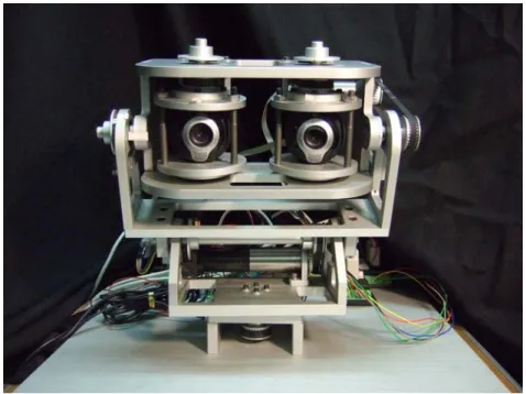
3.1 Humanoid Vision System Description

The HVS is built with two cameras and five motors to emulate human eyeballs as shown in Fig. 3.1. These five motors, FAULHABER DC−servomotors, are used to drive the two cameras to implement the eye movement, one for the conjugate tilt of two eyes, two for the pan of two eyes, and two for the pan and tilt of the neck correspondingly. The control of DC−servomotors is executed by the motion control card, MCDC 3006 S, in a positioning resolution of 0.18°. With these 5 degrees of freedom, the HVS would track the target whose position is determined from the image

processing of the two cameras. In addition, these two cameras, QuickCamTM

Communicate Deluxe, have specifications listed below. [19]

ƒ 1.3-megapixel sensor with RightLight™2 Technology

ƒ Built-in microphone with RightSound™ Technology

ƒ Video capture: Up to 1280 x 1024 pixels (HD quality) (HD Video 960 x 720 pixels)

ƒ Frame rate: Up to 30 frames per second

ƒ Still image capture: 5 megapixels (with software enhancement) ƒ USB 2.0 certified

ƒ Optics: Manual focus

In this proposed system structure, the baseline 2d is set as constant equal to 10.5cm. The control and image process are both implemented in personal computer with 3.62 GHz CPU.

3.2 Depth Detection

3.2.1 Traditional depth detection algorithm

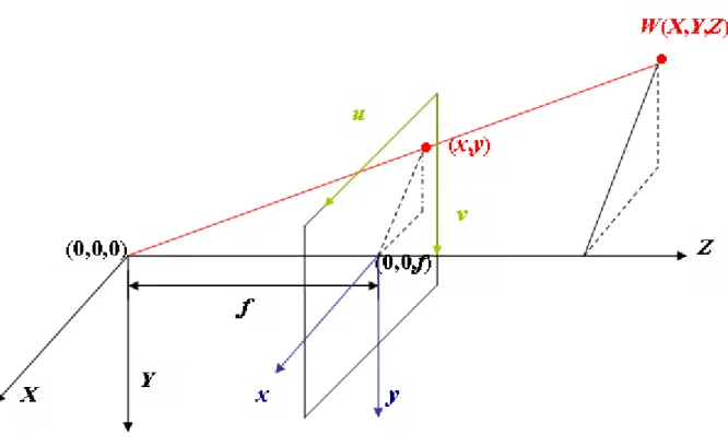
Before introducing depth computing, the triangulation for one camera will be introduced first [20]. Fig. 3.2 illustrates the relation of a world point with world coordinates (X, Y, Z), which is projected onto camera coordinates (x, y) and onto image coordinates (u, v) in the image plane. The mapping between the camera coordinates (x, y) and the world coordinates (X, Y, Z) is formed by means of similar triangles as x f X y Z Y ⎡ ⎤₌ ⎡ ⎤ ⎢ ⎥ ⎢ ⎥ ⎣ ⎦ ⎣ ⎦ (3.1-1)

where f is the focal length of the camera. The origin of the camera frame is located at the intersection of the optical axis with the image plane, while the origin of the image frame is located at the top left corner of the image. The transformation between the image frame and the camera frame is given by

( )

( )

0 0 u v u round k x u v round k y v ⎧ = + ⎪ ⎨ = + ⎪⎩ (3.1-2)

where ku and kv are the scale factors in m−1 of the horizontal and vertical pixels,

respectively. Besides, ( , ) are the image coordinates of the origin of the camera frame and the function round(․) rounds the element to its nearest integer.

0

u v₀

It is known that mapping a 3-D scene onto an image plane is a multiple-to-one transformation, i.e., an image point may represent different locations in world coordinate. To derive the world coordinate information uniquely, two cameras should be used. With thetriangulation theory and the disparity of a pair of corresponding object points in two camera’s frames, the real location of an object can be reconstructed.

Y

L

β

L

β

R

Y

_R

Z

R

Z

S Side View

Z

_L

X

L

θ

θ

L R

X

_R L R 0 0 s

ereo reference fram t

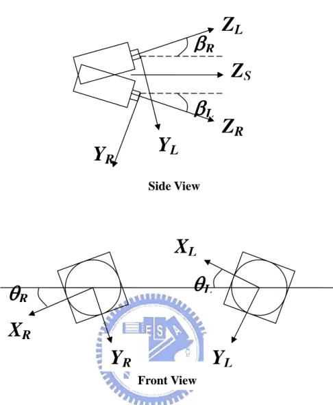
Fig. 3.3 Configuration of a HVS with binocular cameras

A HVS is implemented by two cameras with fixed focal length as shown in Fig. 3.3. The baseline of the two cameras is 2d, where d is the length from the center of baseline to the camera, left or right. Let the pan angles of the left and right cameras be denoted by α and α , respectively. Since the cameras may not be placed precisely, there often exists a small tilt angle 2β and a small roll angle 2φ between two cameras. Choose the stereo reference frame at O , which divides the tilt angle, roll angle, and baseline equally, with Z−axis pointing towards the fixating point F. For the

left camera coordinate frame L, it is related to the st e by a

ranslation vector dL=(−d,0,0) and a rotation matrix ΩL =Ω

(

α β φL, L, L

)

, where

Front View

αL, βL=β0and φL , tilt and roll of frame L

and

=φ0are respectively the Euler angles of pan

(

α β φ, ,

)

Ω

(

)

is the general rotation matrix expressed as

(

)

(

)

(

)

(

)

(

)

(

)

(

)

(

)

(

)

11 12 13 21 22 23 31 32 33 , , , , , , , , , , , , , , , , , , , , ω α β φ ω α β φ ω α β φ α β φ ω α β φ ω α β φ ω α β φ ω α β φ ω α β φ ω α β φ ⎡ ⎤ ⎢ ⎥ = ⎢ ⎥ ⎢ ⎥ ⎣ ⎦ Ω (3.1-3) with φ +sinβ sinφ

sβ sinφ −sinβ cosφ

ω33(α,β,φ)= cosα cosβ

B from frame L to the reference frame

is described as

is the position vector of B in the reference frame. From (3.1-1) and (3.1-4), we have

ω11(α,β,φ)= cosα cosφ

ω12(α,β,φ)= sinα sinβ cosφ −cosβ sinφ

ω13(α,β,φ)= sinα cosβ cos

ω21(α,β,φ)= cosα sinφ

ω22(α,β,φ)= sinα sinβ sinφ +cosβ cosφ

ω23(α,β,φ)= sinα co

ω31(α,β,φ)= −sinα

ω32(α,β,φ)= cosα sinβ

The transformation equation of the object point

(

)

L L s L

p =Ω p −d (3.1-4)

where pL=[XL YL ZL]T is the position vector of B in frame L and ps=[Xs Ys Zs]T

L L L L L L x f X y Z Y ⎡ ⎤ ⎡ ⎤ = ⎢ ⎥ ⎢ ⎥ ⎣ ⎦ ⎣ ⎦ (3.1-5) where

(

) (

11 , 0, 0

)

12

(

, 0, 0

)

13

(

, 0, 0

)

L s L s L s L x = X +d ω α β φ +Yω α β φ +Z ω α β φ

(

) (

21 , 0, 0

)

22

(

, 0, 0

)

23

(

, 0, 0

)

L s L s L s L y = X +d ω α β φ +Yω α β φ +Zω α β φ

(

) (

31 , 0, 0

)

32

(

, 0, 0

)

33

(

, 0, 0

)

L s L s L s L

Z = X +d ω α β φ +Yω α β φ +Zω α β φ

Therefore, the relation between image coordinate of frame L and world coordinates are L u L u round k x u ⎧ = + ⎪ ⎨ (3.1-6)

the right camera coordinate frame R, the transformation equation of B is described as

p =Ω p −d (3.1-7)

T

B in frame =(d,0,0) is th translation vector, and the rotation matrix

(

)

(

)

0 0 L v L v =round k y +v ⎪⎩ Similarly, for

(

)

R R s R

where pR=[XR YR ZR] is the position vector of R, dR e

(

)

R = α β φR, R, R

Ω Ω with α , β =−β0and

lation between the right camera coordinates and the world coordinates are given by

R R

φR=−φ0 being the Euler angles of pan, tilt and roll of frame R, respectively. Using

(3.1-1) and (3.1-7), the re R _R R R R R x f X y Z Y ⎡ ⎤ ⎡ ⎤ = ⎢ ⎥ ⎢ ⎥ ⎣ ⎦ ⎣ ⎦ (3.1-8) where

(

) (

11 , 0, 0

)

12

(

, 0, 0

)

13

(

, 0, 0

)

R s R s R s R x = X −d ω α −β φ− +Yω α −β φ− +Zω α −β φ−

(

) (

21 , 0, 0

)

22

(

, 0, 0

)

23

(

, 0, 0

)

R s R s R s R y = X −d ω α −β φ− +Yω α −β φ− +Zω α −β φ−

(

) (

31 , 0, 0

)

32

(

, 0, 0

)

33

(

, 0, 0

)

R s R s R s R Z = X −d ω α −β φ− +Yω α −β φ− +Zω α −β φ−

Accordingly, the relation between image coordinate of frame R and world coordinates can be express as L u L u round k x u ⎧ = + ⎪ ⎨ (3.1-9)

the disparity of B between the left image

(

)

(

)

0 0 L v L v =round k y +v ⎪⎩

Since the angles β0 and φ0 are small, the absolute value of the terms ω12, ω21, ω23, ω32

for both the left and the right frames are usually much smaller compared to the other terms. Further define stereo disparity, usd, as

frame and right image frame, expressed as

sd L R

u =u − (3.1-10) u

whic

osition vector of B in the left and right camera frames are

L

R (3.1-12)

h will be applied to the determination of the depth of B.

In the HVS, if two cameras are placed precisely in parallel, then the pan, tilt, and roll angles between these two cameras are zeros, i.e., αL=αR =0, βL =βR=β0 =0, and φL

=φR=φ0=0. From (3.1-4) and (3.1-7), the p respectively obtained as

L s

p = p −d (3.1-11)

R s

p = p −d

with Ω_L =Ω_R =I . Based on the same process from (3.1-5) to (3.1-9), the disparity is found as

(

)

(

)

sd L R u L u R

u =u −u =round k x −round k x (3.1-13) Since the term on the right can be approximated as

)

(

u L

)

(

u R L L R R uL u R L R k k Z Z ≈ − round k x round k x f X f X − (3.1-14)

where ZL= ZR= Z, the disparity can be written as

uL sd L R u u u k f XL L ku Rf XR R Z − (3.1-15) Rearranging it leads to = − ≈ uL L L u R R R sd Z u k f X −k f X ≈ (3.1-16)

which gives the depth of B after usd, XL, XR, fL, fR, kuL, and kuL are obtained. In general

case, for arbitrary object point, it is hard to obtain the XL and XR values. Therefore, the

traditional depth computation is usu se er t ssumption that both cameras

have the sam

ally u d und he a

e focal length, i.e., = = , and then (3.1-16) can be

simplified as

uL L

(

)

( )

2 u L R u uL L L u R R R k f X X k f d k f X k f X Z u u u − − ≈ = = (3.1-17) where X sd sd sd

cameras. Clearly, with (3.1-17), only and usd are required to find the depth Z.

3.2

e used to train the system for elim

training algorithm, which is the most commonly adopted for MLP

L−XR=2d is the separation of two k f , u

d

.2 ANN depth detection algorithm

Stereo pair obtained from two cameras can be utilized to compute the depth of a point by using the traditional depth computation introduced in previous section. However, to apply the computation, parameters of each camera need to be experimentally obtained in advance. Therefore, ANN can b

inating the complicate computation process.

It is well known that multilayer neural networks can approximate any arbitrary continuous function to any desired degree of accuracy [14]. A number of investigators have it for different proposes in stereo vision. For example they have been used for camera calibration [15], establishing correspondence between stereo pair based on features [16] and generating depth map in stereo vision [12][15]. In this thesis, a feed forward neural network was used for depth estimation. The ANN computation system doesn’t need to calibrate the cameras in HVS. This can be very helpful in rapid prototyping application. The proposed thesis employs a Multi-Layer Perceptron (MLP) network trained by BP

network.

In the problem, the thesis proposed a multilayer ANN model because camera calibration problem is a nonlinear problem and cannot be solved with a single network [17]. Further, according to the neural network literature [18] more than one hidden layer is rarely needed. The more layers that a neural network have, the more parameter values need to be set because the number of neurons in each layer must be

determined. Therefore, to reduce the number of permutations, a network with one hidd

ctual depth, after training; give the world coordinates for any matched pair of points.

en layer was selected.

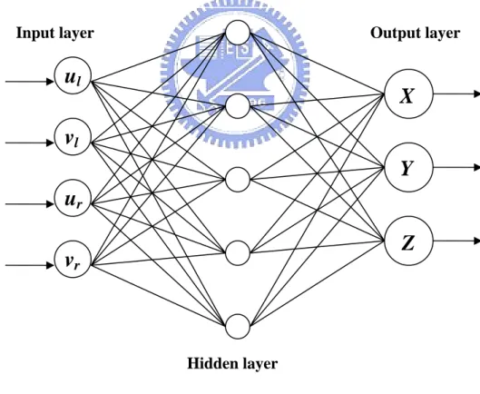
The network model had been used in Fig. 3.4 for simulation consists of four input neurons, five hidden neurons and three output neurons. The input neurons’ corresponding to the image coordinates of matched points found in the stereo images (ul, vl) and (ur, vr). These points are generated by the same world point on both images

and formed the input data for the neural network. The output neurons corresponding to the world coordinates of a point which are mapped as (ul, vl) and (ur, vr) on the two

images. The network is trained in an interesting range of a

Fig. 3.4 ANN model used for this thesis

The algorithm requires training a set of matched image points whose corresponding world point is known. The set of matched points and the world

Y

v

r

u

r

Input layer Output layer

u

l

v

l

Hidden layer

Z

X

coordinates thus obtained and formed the training data set for the ANN. Once the network is trained, we present it with arbitrary matched points and it directly gives us the d

thesis) will be issued in next Chapter for getting more precise detection result.

epth corresponding to the matched pair.

The main problem to using the MLP network is how to choose optimum parameters. Presently, there is no standard technique for automatically setting the parameters of MLP network. That is to say, the best architecture and algorithm for the problem can only be evaluated by experimentation and there are no fixed rules to determine the ideal network model for a problem. Therefore, experiments were performed on the neural network to determine the parameter according to its performance. Parameters with the number of neurons in the hidden layer (one hidden layer is employed in this

Chapter 4

Experimental Results and Discussion

4.1 Experimental Settings

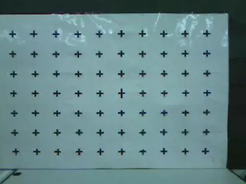
The board consisting of a set of grid points is placed in front of the HVS for depth detection as shown in Fig.4.1 and Fig.4.2, one for the left camera and the other for the right. With the use of these two cameras, the HVS captures images of a specified cross at various distances, ranging from 65 to165 cm. To verify the usefulness of the proposed ANN depth detection algorithm, the experiment is implemented by changing the distance Z between the HVS and the board, where Z starts from 65 cm to 165 cm at an increment of 10 cm.

In the next section, there are different cases used to show the restriction of traditional depth detection algorithm and the flexibility and features of the ANN depth detection algorithm proposed in the thesis.

Fig. 4.1 The board at Z=105cm captured form left camera

4.2 Experimental Results

4.2.1 Restrictions on Traditional depth detection

algorithm

It is known that the traditional depth detection algorithm (3.1-17) is only suitable for the case that both cameras have the same focal length and their optic axes are parallel. However, in practical situation, the two cameras of an HVS generally have a little difference in their focal length or a little deflection between their optic axes. As a result, (3.1-17) is inappropriately used to detect the depth of a scene. To show these restrictions on an HVS, experiments will be set for demonstration.

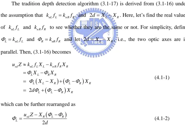
The tradition depth detection algorithm (3.1-17) is derived from (3.1-16) under the assumption that k f_{uL L} =k_{u R}f_R and 2d = X_L−X_R. Here, let’s find the real values

of and to see whether they are the same or not. For simplicity, define

and and let

uL L

k f k_{u R}f_R

L k fuL

Φ = _L Φ_R =k f_{uR R} 2d = X_L−X_R, i.e., the two optic axes are in

parallel. Then, (3.1-16) becomes

(

) (

)

(

)

2 sd uL L L u R R R L L R R L L R L R L L R R u Z k f X k f X X X R X X d X Φ Φ Φ Φ Φ Φ Φ ≈ − = − = − + − = + − X Φ (4.1-1)

which can be further rearranged as

(

)

2 sd R L L u Z X d Φ Φ Φ = − − R (4.1-2) where the baseline 2d is fixed. Next, let’s show the way to calculate for the left

camera in the HVS. By setting the shortest focal length for each camera, which is fixed but not exactly known, two images are obtained in

L

Φ

Fig. 4.5 for Z=95 cm and 2d=10.5 cm. To calculateΦ_L, the term X_R

(

Φ Φ_L− _R

)

in (4.1-2) has to be eliminated. By choosing the same 12 points in both images Fig. 4.5 (a) and (b), enclosed in the

dashed square, the addition of X_R

(

Φ Φ_L− _R

)

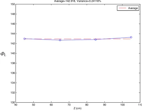
of these twelve points will vanish when they are vertically symmetric to the center line lR in the right image. Hence,

( )

12 1 1 12 2 sd _i L i u Z d Φ = =

∑

(4.1-3)

where (usd)i is the disparity of the i-th point. Fig. 4.3 shows the result of ΦL for

different distance Z from 45 cm to 105 cm to verify that ΦL is around the average

value Φ =142.918 with 0.24116% variation. In a similar way, the value of _L corresponding to the case of the shortest focal length, Z=85 cm and 2d=10.5 cm, can be obtained as R Φ

( )

12 1 1 12 2 sd _i R i u Z d Φ = =

∑

(4.1-4)

where the 12 points are chosen from the images shown in Fig. 4.6, vertically symmetric to the center line lL in the left image. Fig. 4.4 shows the result of ΦR for

different distance Z. It is obvious that Φ is approximate to _L Φ with 0.27821% _R

variation. Since Φ is indeed near to _L Φ , the traditional depth detection algorithm _R

40 50 60 70 80 90 100 110 130 132 134 136 138 140 142 144 146 148 150 Z (cm) Average=142.918, Variance=0.24116% Average ΦL

Fig. 4.3 ΦL for different distance Z from 45 cm to 105 cm

40 50 60 70 80 90 100 110 130 132 134 136 138 140 142 144 146 148 150 Z (cm) Average=143.8118, Variance=0.27821% Average ΦR

(a)

lR

(b)

Fig. 4.5 The same 12 points using to calculateΦ_L for Z=95cm

(a) (b)

Fig. 4.6 The same 12 points using to calculateΦ_R for Z=95cm

lL P1 P2 P1 P2 (a) (b)

Human eyes always focus on the center of entire eyeshot. Based on this characteristic, two adjacent points P1 and P2 in the center line of the training area,

within eyeshot center of HVS, on the experimental board was shown in Fig. 4.7 are chosen as the testing points. P1 and P2 used to acquire test the error between depth

detection result and actual depth.

The average error is computed by mean absolute error that can be written as ˆ

ma

e =mean Z⎡_⎣ −Z ⎤_⎦ (4.1-5) where ema is the mean absolute error of the network. Z and Zˆ denote the depth that

is actually measured and the corresponding depth given by the network respectively. Therefore, to represent distinct situation of ema, four different conditions are schemed

as shown in the Fig. 4.8 to Fig. 4.11. The first case represent two cameras of HVS are placed in parallel with the same focal length. The second case is respect to distinct focal length. The third case is respect to insignificant deflection between optic axes of two cameras. And for the last case distinct focal length and insignificant deflection are included.

Case I 65 75 85 95 105 115 125 135 145 155 165 -10 -8 -6 -4 -2 0 2 4 6 8 10

Traditional depth computation error plot(caseI), (Error range: 0.017387%~1.7834%)

(cm)

(%

)

Average

Fig. 4.8 e_ave of two cameras placed in parallel with the same focal length Case II

65 75 85 95 105 115 125 135 145 155 165 0 5 10 15 20 25 30

Traditional depth computation error plot(caseII), (Error range: 15.1465%~18.9796%)

(cm)

(%

)

Average

Fig. 4.9 e_ave of two cameras with distinct focal length Case III 65 75 85 95 105 115 125 135 145 155 165 100 200 300 400 500 600 700 800 900 1000 1100

Traditional depth computation error plot(caseIII), (Error range: 58.3189%~1145.9954%)

(cm)

(%

)

Case IV 65 75 85 95 105 115 125 135 145 155 165 500 1000 1500 2000 2500

Traditional depth computation error plot(caseIV), (Error range: 155.1946%~2653.9037%)

(cm)

(%

)

Fig. 4.11 of two cameras with distinct focal length and insignificant deflection

ave

e

These figures show that the ema of the actual depth range in 65 to165 cm of case I

is between 0.017387% and 1.7834%, case II is between 15.1465% and 18.9796%, case III is between 58.3189% and 1145.9954% and case IV is between 155.1946% and 2653.9037%. The maximum of percentage error results of these case are greater than 15% except case I. This is mean that the algorithm only is used in the situation similar to case I, or else need to rewrite the formula with more parameter to fit all situation able to appear.

4.2.2 Flexibility of ANN Depth Detection Algorithm

The existence of restrictions on Traditional depth detection algorithm is already confirmed and shown in previous subsection. In order to unrestricted, the ANN depth detection algorithm proposed in this thesis.

The ANN architecture for depth detection will evaluate by experimentation. Here, the number of neuron in the output layer need to be decides first. One case is three neurons which respectively corresponding to the world coordinates (X, Y, Z) of the world object point in the output layer and another one is just one neuron for depth Z. The case IV in the previous subsection is used to treat as the general case in the problem. The training data of the neural network is the same 12 points in left and right of each image, with different distance Z from 65cm to 165cm at an increment of 20cm. To check the accuracy of the trained network, we presented the network with stereo-pair points that were not completely included in the training set but were from within our range of interest of distance. The testing data is the two same points; they are adjacent, as introduced in the previous subsection in the left and right image with different distance Z from 65cm to 165cm at an increment of 10cm. After the training process had finished, each neural network is tested with the training and testing data sets.

Fig. 4.12 shown the ema in each depth simulated from the net that consists of four

input neurons, five hidden neurons and three output neurons. As the diagram indicates, the ema ranges from 0.48455% to 2.4771%. The maximum ema, 2.4771%, represents

the error of its corresponding net. Each different number of neuron creates ten distinct nets and the ema of ten nets shown in Fig. 4.13 with five hidden neurons. The average

of ema from ten nets with the same number of neurons Hn in hidden layer, ema_Hn,

show each ema_Hn with one and three output neurons respectively. It is clearly to find

that the error range of one output neuron is always greater than three output neurons. For accuracy, the three output neuron is chosen in the proposed architecture.

65 75 85 95 105 115 125 135 145 155 165 0.6 0.8 1 1.2 1.4 1.6 1.8 2 2.2 2.4

NN(XYZ)-Error plot, neural number=5, (Error range: 0.48455%~2.4771%)

(cm)

(%

)

1 2 3 4 5 6 7 8 9 10 2.2 2.4 2.6 2.8 3 3.2 3.4 3.6 3.8 training net %

BP(XYZ) minimun error=2.2748% (neural no.=5) Average=2.9542%, Variance=0.23892% Average

Fig. 4.13 ema of ten nets with five hidden neurons

0 5 10 15 20 30 40 50 60 70 80

neural number in hidden layer

%

BP(Z) minimun error=20.3715% (neural number=3 )

error average

0 5 10 15 0 5 10 15 20 25 30 35 40 45 50

neural number in hidden layer

%

BP(XYZ) minimun error=2.9542% (neural number=5 )

error average

Fig. 4.15 Each ema_Hn with three output neurons

After decide the number of output neuron, the number in the hidden layer is proceeded to be resolved. From Fig. 4.15 also tells us that the best choice for neuron number in the hidden layer in the problem is five. Therefore, we may reasonably conclude that the better MLP network architecture for detecting depth should be consists of four input neurons, five hidden neurons and three output neurons.

In order to eliminate the net that doesn’t train the training data successfully, a threshold value T of ema from training data need to be set. If the ema form training data

of the net is large than T, the net will not be enrolled. The setting value H must be large than the ema from training data such that the network could.

The error results can be seen for different case introduced in subsection from proposed net is shown from Fig. 4.16 to Fig. 4.19. They can be noted that even in the worst case, the error in depth computation was still well below 4%.

Case I 1 2 3 4 5 6 7 8 9 10 0.8 1 1.2 1.4 1.6 1.8 2 2.2 2.4 2.6 2.8 training net %

BP(XYZ) minimum error=1.9753% (neural no.=5) Average=2.2439%

Average for ANN Average for tradition

Fig. 4.16 Each ema_Hn from proposed net of Case I

1 2 3 4 5 6 7 8 9 10 0 2 4 6 8 10 12 14 16 18 training net %

BP(XYZ) minimum error=1.7435% (neural no.=5) Average=2.1169%

Average for ANN Average for tradition

Fig. 4.17 Each ema_Hn from proposed net of Case II

Case III 1 2 3 4 5 6 7 8 9 10 1.4 1.45 1.5 1.55 1.6 1.65 1.7 1.75 1.8 1.85 training net %

BP(XYZ) minimum error=1.4234% (neural no.=5) Average=1.5368%

Fig. 4.18 Each ema_Hn from proposed net of Case III Case IV 1 2 3 4 5 6 7 8 9 10 2.2 2.4 2.6 2.8 3 3.2 3.4 3.6 3.8 training net %

BP(XYZ) minimum error=2.2748% (neural no.=5) Average=3.2395%

Average for ANN

Fig. 4.19 Each ema_Hn from proposed net of Case IV

The training data is obtained from stereo pair manually. The reason for decreasing the number of inputs was to determine whether the desired depth values could still be achieved with acceptable accuracy. Therefore, if the training data is only obtained from Z=65 and 165cm, the testing error average is 53.0081% as shown in Fig. 4.20. Fig. 4.21 and Fig. 4.22 are shown the testing error of training data is obtained from Z=65, 115, 165cm and Z=65, 95, 135, 165cm respectively. The Fig. 4.22 indicates that the training data with four distinct depths can get the result with error around 5%.

1 2 3 4 5 6 7 8 9 10 20 30 40 50 60 70 80 90 100 training net %

BP(XYZ) minimun error=21.7075% (neural no.=5) Average=53.0081%, Variance=82.5972% Average

Fig. 4.20 The testing error of training data is obtained from Z=65 and 165cm

1 2 3 4 5 6 7 8 9 10 10 15 20 25 30 35 40 45 50 55 training net %

BP(XYZ) minimun error=12.3236% (neural no.=5) Average=31.1636%, Variance=65.2786% Average

1 2 3 4 5 6 7 8 9 10 2 4 6 8 10 12 14 16 training net %

BP(XYZ) minimun error=2.9263% (neural no.=5) Average=5.412%, Variance=187.9889% Average

Fig. 4.22 The testing error of training data is obtained from Z=65, 95, 135, 165cm The algorithm is different form traditional detection depth algorithm in the sense that no extrinsic or intrinsic camera parameters are found for any of the camera. The system is trained such that it learns to directly find the depth of objects.

Chapter 5

Conclusion

The proposed algorithm in this thesis has shown that it is possible to use a neural network to compute actual depth with good accuracy. The thesis used an ANN to train the system such that, when the system is presented with a matched pair of points, it automatically computes the depth of the corresponding object point. The algorithm differs from traditional depth detection algorithm to the problem. That is, there are restrictions for using Traditional depth detection algorithm and the network is trained to compute the correct depth of two matched points without any calibration. The algorithm that is used in this thesis is very simple in concept, independent of the camera model used and the quality of image obtained and yields very good results.

The experimental results in the thesis show that an acceptable accuracy can be obtained but it seems that is not very easy to reach high accuracy by using only neural networks. Neural networks have a good generalization capability in the range that they are trained.

If the depth of the world object can easy be obtain from the HVS, the HVS can be applied to an autonomous mobile robot using stereo vision for navigation, real time track nearest object in front region or locate the interesting object.

The future work for the learning algorithm is to simulate human learning behavior. Just like human learning structure, the learning network will learn in turn stroke by stroke, not in case of learn once for all.

Reference

[1] M. Waldowski, “A new segmentation algorithm for videophone applications based on stereo image pairs,” IEEE Trans. Commun., vol. 39, pp. 1856–1868, 1991.

[2] D. Kauffman and S. Wood, “Digital elevation model extraction from stereo satellite images,” in Proc. Int. Geoscience and Remote Sensing Symp., vol. 1, pp. 349–352, 1987.

[3] J. Rodr´ıguez and J. Aggarwal, “Matching aerial images to 3-D terrain maps,”

IEEE Trans. Pattern Anal. Machine Intell., vol. 12, pp. 1138–1150, 1990.

[4] H. Antonisse, “Active stereo vision routines using PRISM3,” in Proc. SPIE–Int.

Soc. Opt. Eng., vol. 1, pp. 745–756, 1993.

[5] W. Poelzleitner, “Robust spacecraft motion estimation and elevation modeling using a moving binocular head,” in Proc. SPIE- Int. Soc. Opt Eng., vol. 1829, pp. 46–57, 1993.

[6] K. Nishihara and T. Poggio, “Stereo vision for robotics,” in Proc. Robotics

Research, First Int. Symp., pp. 489–505, 1984.

[7] N. Ayache and F. Lustman, “Trinocular stereo vision for robotics,” IEEE Trans.

Pattern Anal. Machine Intell., vol. 13, pp. 73–85, 1991.

[8] Y. Matsumoto, T. Shibata, K. Sakai, M. Inaba, H. Inoue, "Real-time Color Stereo Vision System for a Mobile Robot based on Field Multiplexing," in IEEE

Int. Conf. on Robotics and Automation, pp.1934-1939, 1997.

[9] S. B. Goldberg, M. W. Maimone, L. Matthies, "Stereo Vistion and Eover Navigation Software for Planetary," in IEEE Aerospace Conference, 2002.

[10] E. Huber, D. Kortenkamp, "Using Stereo Vision to Pursue Moving Agents with a Mobile Robot," in IEEE Conference on Robotics and Automation, 1995. [11] Y. Mokri, M. Jamzad, "Omni-stereo vision system for an autonomous robot

using neural networks," in Electrical and Computer Engineering, 2005. [12] Q. Memony, S. Khanz, "Camera calibration and three dimensional world

reconstruction of stereo-vision using neural networks," International Journal of

Systems Science, vol. 32, pp. 1155-1159, 2001.

[13] R. Mohr, L. Quan, F. Veillon, "Relative 3D Reconstruction Using Multiple Uncalibrated Images," International Journal of Robotics Research, vol. 14, pp. 616-632, 1995.

[14] K. I. Funahashi, "On the approximate realization of continuous mapping by neural networks," in Neural Networks. vol. 2, pp. 183-192, 1989.

[15] Y. Do, "Application of neural networks for stereo camera calibration," in

International Joint Conference on Neural Network, 1999.

[16] C. Y. Choo, N.M. Nasrabadi, "Hopfield network for stereo vision

correspondence," in Neural Networks, IEEE Transactions on. vol. 3, pp. 5-13, 1992.

[17] L. Fausett, Fundamentals of Neural Networks: Architectures, Algorithms And

Applications, Prentice-Hall Inc, 1994.

[18] Department of Trade and Industry, Best Practice Guidelines for Developing Neural Computing Applications, pp86-87, 1994.

http://www.logitech.com/index.cfm/home [19]

[20] W. Y. Yau, H. Wang, "Fast Relative Depth Computation for an Active Stereo Vision System," Real-Time Image, pp.189-202, 1999.