噪訊增強的無線通訊網路盲蔽式錯誤率估測器之設計與效能分析

國 立 交 通 大 學

電信工程研究所

博 士 論 文

噪訊增強的無線通訊網路盲蔽式錯誤率估

測器之設計與效能分析

Design and analysis of noise-enhanced blind

error rates estimation in wireless network

研 究 生：劉人仰

指導教授：蘇育德 博士

噪訊增強的無線通訊網路盲蔽式錯誤率估測器之

設計與效能分析

Design and analysis of noise-enhanced blind error

rates estimation in wireless network

研究生：劉人仰

Student:

Jen-Yang

Liu

指導教授：蘇育德 博士 Advisor:

Dr.

Yu

T.

Su

國立交通大學

電信工程研究所

博士論文

A Dissertation

Submitted to Institute of Communication Engineering

College of Electrical and Computer Engineering

National Chiao Tung University

in Partial Fulfillment of the Requirements

for the Degree of Doctor of Philosophy

in

Communication Engineering

Hsinchu, Taiwan

i  噪訊增強的無線通訊網路盲蔽式錯誤率估測器之設計與效能分析   研究生：劉人仰      指導教授：蘇育德  博士  國立交通大學電信工程研究所  中文摘要    基於多筆資訊做資料偵測或融合的技術已經廣泛被使用在通訊系統上。本論 文考慮一廣義的無線網路框架，在此框架中，我們假設訊號會經過不同的鏈結 (link)到達接收器，而鏈結的種類包含了直接鏈結(從傳送端到接收端)以及兩步 (two‐hop)鏈結(從傳送端經由中繼站到達接收器)。在兩步鏈結中，中繼端會把收 到的訊號作解碼並傳送重新編碼過後的訊號到接收端。在此框架中，資料偵測或 融合的技術通常需要各鏈結的錯誤率資訊。舉例來說，在二元相位調變(binary  phase‐shift keying)合作式通訊系統中，最佳資料偵測需要知道遠端鏈結(從傳送端 到中繼站的鏈結，縮寫為 SR 鏈結)的錯誤率資訊。同樣地，在資料融合中心(fusion  center)，基於多感測測量值的最佳資料融合也是需要各遠端鏈結的錯誤率資訊。  為了在接收端盲蔽式地估測遠端的二進位調變(binary modulation)錯誤率，我 們首先把估測問題轉換成解非線性聯立方程式的問題。每一個方程式皆反映成功 匹配機率(success matching probability)和兩鏈結的錯誤率關係。其中，我們定義 成功匹配機率是給定一傳送訊號下兩鏈結做出相同決策的機率。為了要讓此非線 性聯立方程式有解，其基本的要求是要有足夠的鏈結數目。當鏈結數目不夠時， 我們需要部分的資訊才能求出解，部分的資訊可能包含了從傳送端到接收端的鏈 結(SD 鏈結)錯誤率或是從中繼站到接收端的鏈結(RD 鏈結)錯誤率。而事實上，我 們發現當我們沒有從中繼站到接收端的鏈結錯誤率資訊時，即使有再多的鏈結數 目亦是無法求出合理解來，這是因為從傳送端經中繼站到接收端的錯誤率會是 SR 鏈結和 RD 鏈結錯誤率的對稱函數。 

ii  為了解決上述的問題以及增加收斂速度，我們提出基於蒙地卡羅 (Monte‐Carlo)的估測器。具體來說，我們在接收端加入噪訊(noise)到接收訊號。 在第一種方式中，我們加入噪訊是為了產生虛擬的 SD 鏈結或是 RD 鏈結，藉由 這樣的方法，我們可以在即使只有一中繼站情況下亦可以得到有解的非線性聯立 方程式問題。此方法我們稱為虛擬鏈結估測器(virtual link aided estimatior)。在第 二種方法中，我們加入噪訊使得收到訊號的機率分佈作改變，藉由機率分佈的改 變可以使得估測器的效能有所改善。  事實上，第二種方法顯示出隨機震盪（stochastic resonance）的現象，也就 是說注入適當的噪訊可以改善均方根估測誤差（mean squared estimation error）， 此外我們發現到存在最佳的注入噪訊量使得估測效能最佳。針對此現象，我們做 了一系列的分析並找出最佳的注入噪訊量為何，並藉由模擬驗證我們分析的正確 性。模擬結果也顯示出訊號偵測器配合提出的盲蔽式估測器會和最佳偵測器有差 不多的錯誤率效能。  對於非二進位調變通訊網路，成功匹配機率和鏈結符碼錯誤率(symbol error  rate)的關係不再成立，因此，上述提到的方法不再能夠直接使用於此情況。在參 考文獻[34]中，此問題被轉換成一個非線性最佳化問題，雖然其問題理論上可以 解，但是其複雜度會非常的高如果中繼站數目或是 M‐ary  調變的 M 值不小的時 候。針對此問題，我們基於二位元表示法提出次佳的接收機以及其對應所需的錯 誤率估測器。由於我們可以找到解的數學表示式，其複雜度會遠比上述所提的方 法還要低得多。為了進一步改善偵測器的收斂速度，我們亦提出一噪訊增強的估 測器。模擬的結果顯示我們提出的偵測器伴隨相對應的估測器會和最佳估測器有 相似的效能。在均方估測錯誤(mean square estimation error)效能的評估上，我們亦 可以觀察到隨機震盪的現象 

Design and analysis of noise-enhanced blind error

rates estimation in wireless networks

Student : Jen-Yang Liu Advisor : Y. T. Su

Institute of Communications Engineering National Chiao Tung University

Abstract

Data detection or fusion based on multiple received copies containing the same information arises in many applications. We consider the scenario that each copy is transmitted from the same source through a different wireless link to the same destina-tion node (DN). These links include single-hop, direct source-to-destinadestina-tion (SD) links and two-hop links that require an intermediate decode-and-forward (DF) node to relay the source signal. Detection or fusion under such a circumstance often need channel side information (CSI) about the link reliability. For example, maximum likelihood (ML) detection of binary modulated signals in a DF based cooperative communication net-work (CCN), information about the bit error rates (ERs) of the hidden source-relay (SR) links is needed. Similarly, optimal data fusion based on multiple sensor measurements requires that the ERs of various SR links be available at the fusion center.

To estimate multiple ERs blindly at the DN in a binary modulated network, we convert the estimation problem into one of solving a system of nonlinear equations. Each equation arises from the fact that the success matching probability (SMP) that a bit transmitted over two independent links connecting the same source and destination results in identical destination decisions is nonlinearly related to the ERs of the two associated links. However, the number of distinct link pairs must be larger than the

number of ERs to be estimated so that the system is not an underdetermined one. Various degrees of channel side information (CSI) about the ERs of the SD and relay-destination (RD) links is called for to remove the ambiguity arising from the insufficient number of links in the network and from that due to the symmetric nature of a cascaded source-relay-destination (SRD) link’s ER as a function of its component SR and RD links’ ERs.

We propose novel Monte-Carlo-based estimators that overcome all these shortcom-ings and accelerate the convergence speed. Our proposals involve injecting noise into the samples received by the DN. The injected noise in the first solution, called the virtual link aided (VLA) estimator, help creating virtual SD and RD links to release all CSI requirements, resolve the symmetric ambiguity and provide estimates for ERs of all com-ponent links. Using multitude of VLs, we can enhance the VLA scheme’s performance and reduce the number of RNs required. The role the injected noise plays in another solution, called the importance-sampling-inspired (ISI) estimator, is different: it is used to modify link output statistics to improve the VLA estimator’s convergence rate.

The latter approach exhibits a stochastic resonance effect, i.e., its mean squared estimation error (MSEE) performance is enhanced by injecting proper noise, and there exists an optimal injected noise power level that achieves the maximum improvement. The stochastic resonance effects are analyzed, and numerical examples are provided to display our estimators’ MSEE behaviors, as well as to show that the ER performance of the optimal detector using the proposed estimators is almost as good as that with perfect ER information.

For nonbinary modulation based networks, a relation between the SMP of a link pair and the associated symbol error rates does not exist, hence the nonlinear system based moments approach is not directly applicable. A nonlinear optimization approach which we call LJW blind estimator [34] had been proposed. Unfortunately it requires prohibitively high computational complexity unless M (the modulation order) and the

relay numbers are small. We propose a suboptimal detector based on bit-level represen-tation and a corresponding blind estimator to estimate the error rate of sensor nodes. The complexity of our estimator is much lower than that of LJW as we are able to obtain a closed-form salutation instead of employing an iterative algorithm for solving a nonlinear optimization. To further improve the convergence rate, we propose a noise-enhanced estimator. Simulation results show that the proposed suboptimal detector using the proposed blind estimator render negligible performance loss with respect to that of the optimal detector. A stochastic resonance phenomenon is observed in the estimator’s mean square estimation error performance.

誌 謝

首先感謝我的指導教授 蘇育德 教授，謝謝教授在學術上的

諄諄

教誨，讓我能夠進一步體會到通訊系統的博大精深之處以及箇中樂

趣，也感謝老師在生活上的幫忙，讓我能夠減經家裡的負擔而不需要

為生活而憂愁。此外也感謝各口試委員的建議使得本論文能夠更加完

善。

當然，我也要深深感謝 811 實驗室歷年來的學長姐和學弟妹。尤

其是李昌明 學長，感謝您的分享讓我能夠在這研讀博士的期間留下

美好的回憶。也感謝繃帶小孩的陪伴，沒有你的存在，我想我應該會

在中途就放棄學位吧。

最後也是最重要的是我要感謝我的家人，感謝你們願意讓我專心

研讀博士，包容我這任性的要求，這陣子真的是辛苦你們了。

Contents

Chinese Abstract i

English Abstract iii

Acknowledgements vi

Contents vii

List of Figures x

List of Tables xiv

List of Notations xv

1 Introduction 1

1.1 Stochastic resonance . . . 1 1.2 Motivation and dissertation overview . . . 3

2 Adaptive blind data detection in cooperative communication network 8

2.1 System model, ML detection and blind ER estimator . . . 8 2.2 Side-Information-Aided Blind Single ER Estimation . . . 11 2.3 Multiple-Relay-Aided Blind Multiple ER Estimation . . . 13

3 Blind Multiple ERs Estimation using Virtual Links 17

3.2 Virtual link methods . . . 18

3.3 Blind ER Estimation for BFSK and DPSK Signals . . . 22

3.4 Simulation Results . . . 24

4 Noise-Enhanced ER Estimations 31 4.1 Convergence consideration and a simple variance reduction method . . . 31

4.2 A brief introduction to importance sampling . . . 32

4.3 An importance sampling inspired noise-enhanced estimator . . . 35

4.4 Properties and performance analysis of the noise-enhanced estimator . . 39

4.5 Numerical Results . . . 48

5 Data fusion and blind multiple error rate estimation in a non-binary modulation based wireless sensor network 54 5.1 System model and optimal detector . . . 55

5.2 LJW blind ER estimator . . . 56

5.3 Optimal/suboptimal fusion rules for nonbinary signals . . . 57

5.4 Blind symbol/bit ERs estimator . . . 59

5.5 Noise-enhanced ER estimations . . . 64

5.6 Simulation results . . . 70

6 Conclusions and future work 78 Appendix A 80 A.1 Derivation of (2.6) . . . 80

A.2 Derivations of (2.8) and (2.10) . . . 81

A.3 Proof of Lemma 2.1 . . . 82

A.4 Proof of Lemma 2.2 . . . 83

Appendix B 85 B.1 Derivation of (4.16) . . . 85 B.2 Proof of Lemma 4.1 . . . 85 B.3 Proof of (4.20) . . . 86 B.4 Proof of Theorem 4.2 . . . 87 B.5 Proof of Lemma 4.3 . . . 89 B.6 Proof of Theorem 4.4 . . . 90 B.7 Proof of Lemma 4.6 . . . 91 Bibliography 95

List of Figures

1.1 Example of optimal and suboptimal decision boundary . . . 2 1.2 A wireless multiple-relay network. . . 3 3.1 Ambiguity problem can be solved if the knowledge erd = e is available. . 18

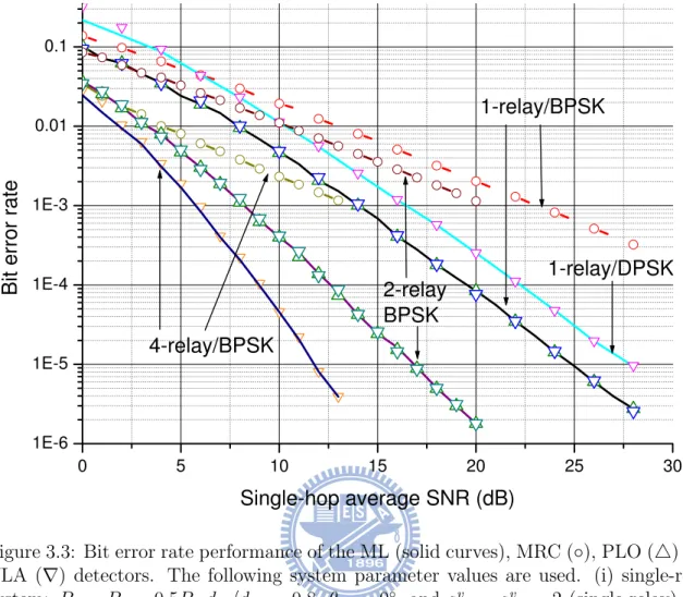
3.2 Block diagram of the maximum likelihood (ML) detector. . . 25 3.3 Bit error rate performance of the ML (solid curves), MRC (◦), PLO (△)

and VLA (∇) detectors. The following system parameter values are used. (i) single-relay system: Ps = Pr = 0.5P , dsr/dsd = 0.8, θsr = 0◦, and av

sd = avrd = 2 (single-relay), (ii) 2-relay system: dr1d = dsr2 = 7/10,

θsr1 = θsr2 = 0◦, Ps = 0.5P, Pr1 = Pr2 = 0.25P , and θ = 45◦, (iii) 4-relay

system: dsd = 10, dsr1 = 5, θsr1 = 45◦, dsr2 = 6, θsr2 = 30◦, dsr3 = 4, θsr3 =

60◦, dsr4 = 5, θsr1 = 0◦, Pp = 0.5P, Pri = 0.125P , for i = 1, 2, 3, 4 and

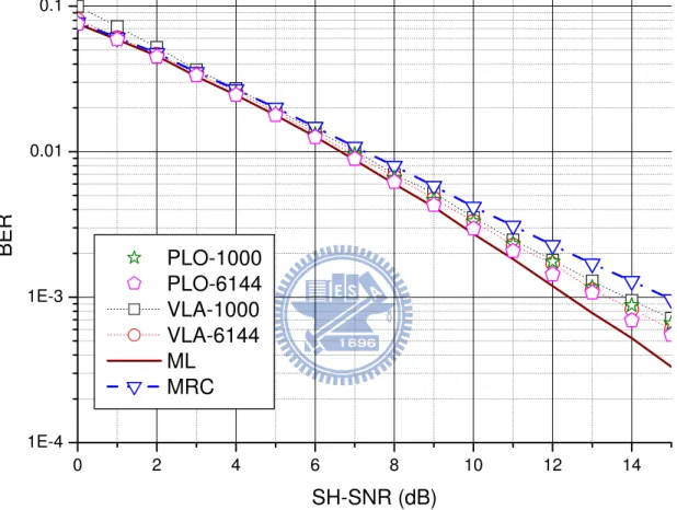
θ = 30◦. . . 27 3.4 Bit error rate performance of the ML, MRC, PLO, and VLA detectors.

The following system parameter values are used. Single-relay system:

Ps = Pr = 0.5P , dsr/dsd = 0., θsr = 45◦, and avsd = avrd = 2. . . 28

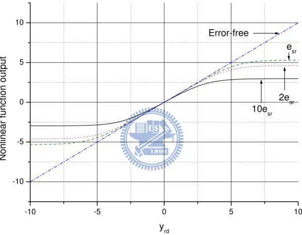
3.5 The nonlinear function (2.3) under various ERs. The system parameter values are Ps = Pr = 0.5P , dsr/dsd = 0., θsr = 45◦ and SNR= 8 dB

(esr = 0.0049). . . . 29

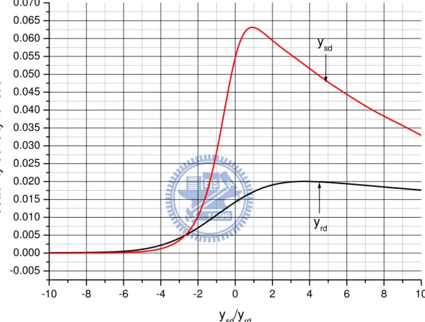
3.6 The probability density functions of ysd and yrdgiven x = 1 in single-relay

system. The system parameter values are Ps = Pr = 0.5P , dsr/dsd = 0., θsr = 45◦ and SNR= 8 dB. . . 30

4.1 The flowchart of the proposed noise-enhanced estimation for data-aided BPSK system in Rayleigh fading channel . . . 37 4.2 Normalized MSEE performance of the noise-enhanced estimator for

data-aided point-to-point BPSK communication in Rayleigh fading channel. The channel quality is 30 dB (error rate e = 2.5× 10−4). The sample size is 10000. . . 49 4.3 Normalized MSEE performance of the ISI-VLA scheme for (a) various

binary modulated 3-link networks (e1 = 0.003, e2 = 0.002, e3 = 0.001; the injected noise power is such that SH SNR=2 for link 1 and e(w)₁ =

e(w)₂ = e(w)₃ ) and (2) BPSK-based single-relay CCN (esr = 0.02922, erd=

0.001988, esd = 0.04356, a (v) sd = a (v) rd = 2, a (w) sd = 1 and a (w) rd = 30).

For 3-link networks, only the performance of be1 is shown. The analytic predictions (solid curves) for these two scenarios are based on (4.23) and (4.42)–(4.44), respectively. . . 50 4.4 Normalized MSEE performance of VLA, VLA-EM, and EISI-VLA schemes

in a BFSK-based single-relay CCN with esr = 0.0127, erd= 5.0711× 10−5

and esd = 0.0298. Other parameter values used are: a

(v)

sd = a

(v)

rd = 2,

e(w)_sd = e(w)_rd = 0.05 and nvl = 30. . . 51

4.5 MSEE reduction ratio (γ) performance of the ISI-VLA estimator with BFSK modulation and a(v)_sd = a(v)_rd = 2. Part (a) is obtained by assuming

dsr = 5, SH-SNR=25 dB with the path loss exponent = 2 (which leads to esr = 0.0016, erd = 0.0016, esd = 0.0062). Part (b) assumes that dsr = 8,

SH-SNR=18 dB with path loss exponent = 4 so that esr = 0.0127, erd=

5.0711× 10−5, esd = 0.0298. The MSEE reduction ratio of the RD link is

4.6 MSEE reduction ratio behavior of the EISI-VLA estimator for BFSK based CCN with different nvl. Other system parameter values are the

same as those of Fig. 4.5(b). . . 53

5.1 Parallel distributed detection system . . . 55

5.2 A binary symmetric channel with parameter e . . . . 58

5.3 A binary nonsymmetric channel with parameter e0 _{and e}1 _{. . . . 60}

5.4 16-QAM with Gray mapping labelling . . . 65

5.5 16QAM error rate in Rayleigh fading with α = 2. . . . 67

5.6 Bit (symbol) error rate performance of various detectors with QPSK/16-QAM (MFSK) modulation and Gray mapping labelling. The qualities of the three links for QPSK modulation are denoted by ( Eb N0, Eb N0 + 1, Eb N0 + 2 ) in dB. Similarly, ( Eb N0, Eb N0 + 2, Eb N0 + 4 ) and (SNR,SNR+3,SNR+6) are the link qualities for QAM and 4-FSK, respectively. . . 72

5.7 Normalized MSEE performance of blind bit-level estimator in a 16-QAM-based three link wireless sensor network. The qualities of these three links are 10, 15, and 20 (dB), respectively. . . 73

5.8 Normalized MSEE performance of blind symbol ER estimator in a 4-FSK-based three link wireless sensor network. The qualities of these three links are 15, 20, and 25 (dB), respectively. . . 74

5.9 MSEE reduction ratio behavior of the noise-enhanced estimator in three links sensor network with 16-QAM modulation and Rayleigh fading chan-nel. The qualities ( Eb N0 ) of these three links are 30, 35, and 40 (dB). Noise are injected into the three links such that all links have the same Eb N0 (w) . . 75

5.10 MSEE reduction ratio behavior of the noise-enhanced estimator in three links sensor network with 16-QAM modulation and Rayleigh fading chan-nel. The qualities

(

Eb

N0

)

of these three links are 30, 35, and 40 (dB). We inject noise into the first link

(( Eb N0 ) = 30 (dB) )

such that the quality of the link is Eb

N0

(w)

. We keep the difference of the quality of these three links. That is, the other two links with noise injection have the quality

Eb N0 (w) + 5 and Eb N0 (w) + 10 (dB). . . 76 5.11 MSEE reduction ratio behavior of the noise-enhanced estimator in three

links sensor network with 4-FSK modulation and Rayleigh fading channel. The qualities

(

Eb

N0

)

of these three links are 30, 35, and 40 (dB). We inject noise into the first link

(( Eb N0 ) = 30 (dB) )

such that the quality of the link is Eb

N0

(w)

. We keep the difference of the quality of these three links. That is, the other two links with noise injection have the quality Eb

N0 (w) + 5 and Eb N0 (w) + 10 (dB). . . 77

List of Tables

2.1 A blind ER estimation algorithm for a multiple-relay CCN with knowledge of erkd. . . 15

3.1 A blind ER estimation algorithm for BPSK modulation. . . 22 3.2 The required CSI and the solutions of nonlinear systems under various

modulations. . . 24 3.3 A blind ER estimation algorithm for BFSK/DPSK modulation. . . 24 4.1 A noise-enhanced ER estimation algorithm for data-aided BPSK system

in Rayleigh fading channel. . . 38 4.2 A unified blind noise-enhanced ER estimation algorithm. . . 40 5.1 A blind ER estimation algorithm for high order modulation in sensor

network. . . 62 5.2 The bisection method for finding η = Eb

N0. . . 68

5.3 A noise-enhanced blind ER estimation algorithm for high order modula-tion in sensor network. . . 69

List of Notations

Symbol Meaning

eik

j Probability that fuscion center makes decision Hk based on

the reporting of the jth sensor given Hi is true esd ER of the link from SN to DN

besd Estimate of esd

e(v)_sd ER of the link from virtual SN to DN

e(w)_sd ER of the noise-enhanced link from SN to DN

esrk ER of the link from SN to the kth RN

besrk Estimate of esrk

er_kd ER of the link from the kth RN to DN e(v)_r

kd ER of the link from the virtual kth RN to DN

e(w)_rd ER of the noise-enhanced link from RN to DN berkd Estimate of erkd

esrd End-to-end ER through a RN

fT(z; ε) Nonlinear function of the optimal detector in CCN

hsd Channel coefficient of the SD link

hsrk Channel coefficient of the link from SN to the kth RN

hr_kd Channel coefficient of the link from the kth RN to DN L Number of sensor/relay nodes

N Number of samples

Symbol Meaning

P_bpsk ER for BPSK modulation

P_bdpsk ER for DPSK modulation

P_bbf sk ER for BFSK modulation

Ps Transmission power of SN

Prk Transmission power of the kth RN

psk Success (matching) probability of bysd and byrkd

bpsk Estimate of psk

pkl Success (matching) probability of byrkd and byrld

bpkl Estimate of pkl bp(vs)r Estimate of Pr(by (v) sd =byrd) bps(vr) Estimate of Pr(bysd =by (v) rd) bp(vs)(vr) Estimate of Pr(by_sd(v) =by_rd(v))

q0(·), qk(·) Weight function of the optimal detector in CCN

Qk End-to-end ER through the kth RN

Q(v)_k End-to-end ER through the virtual kth RN b

Qk Estimate of Qk

Q(x) Gaussian Q-function defined by ∫_x∞√1

2πexp (−y

2_{/2) dy}

Q(x, y, ρ) Bivariate Gaussian distribution function defined by √1/2π 1−ρ2 ∫_∞ x ∫_∞ y exp [ −x2 1+y21−2ρx1y1 2(1−ρ2₎ ] dy1dx1 ysd Signal from SN to DN bysd Hard decision of ysd

ysrk Signal from SN to the kth RN

yrkd Signal from the kth RN to DN

y(v)_r

kd Virtual signal from the kth RN to DN

Chapter 1

Introduction

1.1

Stochastic resonance

In signal processing and communication systems, noise is usually the main factor of degrading the system performance. Hence, we always remove the noise either by filter or by some signal processing algorithms. For example, we can improve the quality of a image if we use some denoising algorithm (such as the median filter [1]). However, noise can do improve a system performance in some situations [2]-[17] and we call this phenomenon as stochastic resonance or noise benefit. This phenomenon does not only appear in signal processing or communication systems. It also occurs in the field of sensory neurons [8], circuits and measurement [7]. For the detail and other applications, the reader can refer to [9] and [10].

To realize the stochastic resonance, we consider a very simple example discussed in [11]. Consider an equal priori binary hypothesis testing problem, where x is drawn according to the zero mean Gaussian distribution with variance 1 under H0. Under H1,

x obeys the Gaussian distribution with mean 1 and variance 1. It is easy to show that

the optimal decision boundary is x = 0.5. However, we consider the suboptimal decision boundary: x = 0, as shown in Fig. 1.1. Without changing the detector structure, a simple way to improve the performance is to add a constant signal -1/2 to the received signals. This is equivalent to shift the suboptimal decision boundary to the optimal one and we have the best performance. This procedure can be viewed as a transformation

of the received signals. In [11], a transformation g(x) is also proposed to achieve the performance of the optimal detector, where

g(x) =

{

x for x≥ 1/2 and x < 0

−x for 0≤ x < 1/2

This simple example illustrates two concepts. First, adding a proper noise (it is -1/2 in this example) can improve the performance of suboptimal detector (stochastic resonance effect). Second, a (nonlinear) transformation can also benefit and can be thought as a generalization of stochastic resonance. Hence, it may exist several ways to improve the performance. In this dissertation, we focus on the first type: adding noise.

˃

˃ˁˈ

˦̈˵̂̃̇˼̀˴˿ʳ

˷˸˶˼̆˼̂́ʳ˵̂̈́˷˴̅̌

ˢ̃̇˼̀˴˿ʳ˷˸˶˼̆˼̂́ʳ

˵̂̈́˷˴̅̌

Figure 1.1: Example of optimal and suboptimal decision boundary

Several different performance measurement are used to express the stochastic reso-nance. For example, the performance measurement is error rate in the above example. It is also possible to use signal-to-noise ratio (SNR) [12]. Other possible performance mea-surements are Cram´er-Rao lower bound (CRLB) [13], mutual information [14], Fisher information [15] and correlation [16]. In fact, a good measurement in a system may not be a good one in another system. [17] indicates that it is more useful to measure variations instead of SNR in biology, for instance. It seems that there is no unified performance measurement for all systems to investigate the stochastic resonance. Here, the performance measurement is the mean square estimation error (MSEE), which is

widely used in estimation problem.

1.2

Motivation and dissertation overview

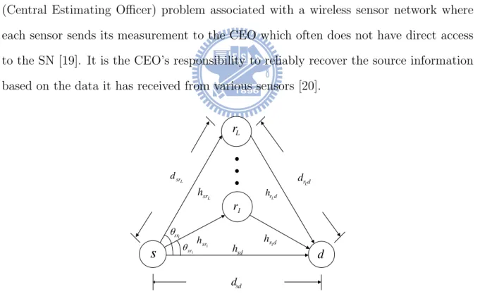
We consider the basic scenario illustrated in Fig. 1.2 where the destination node (DN)

d receives sequences originated from the same source node (SN) s via multiple (L)

flat-fading links. These links may include a direct single-hop (SH) source-destination (SD) link and indirect two-hop links, each connecting the SN and DN with the help of an intermediate relay node (RN), say rk. Such a scenario occurs, for example, in a

cooperative communication network (CCN) in which the SD communication is aided by single or multiple relays which act as virtual antennas to allow resource sharing and provide spatial diversity gains [18]. Another popular example is the so-called CEO (Central Estimating Officer) problem associated with a wireless sensor network where each sensor sends its measurement to the CEO which often does not have direct access to the SN [19]. It is the CEO’s responsibility to reliably recover the source information based on the data it has received from various sensors [20].

1 sr h L sr h sd h d r h 1 d rL h 1 sr T L sr T sd d L sr d d rL d

s

Figure 1.2: A wireless multiple-relay network.

For convenience of subsequent discourse, we define a single-relay CCN as one which consists of a source, a relay (or sensor) and a destination nodes only. We refer to the

associated SD, source-relay (SR) and relay-destination (RD) links as component links and the indirect source-relay-destination (SRD) link as cascaded link. Although many sensing-relay schemes have been proposed, we only consider the Decode-and-Forward (DF) scheme [18]-[26] for which a RN (sensor) demodulates/decodes the received signal from the SN and re-modulates/re-encodes the decoded bit stream before re-transmitting. Since a sensor or cooperative RN may erroneously detect or sense its received signal, conventional maximum ratio combing (MRC) or similar fusion rule is no longer optimal for the DN. In fact, data fusion of various kinds in the presence of imperfect DF relays [24]-[26] and relay selection in a DF-based CCN [27] all require some forms of channel state information (CSI). Depending on the modulation used, the required CSI includes short-term CSI (ST-CSI) like instantaneous link gains and signal-to-noise ratios (SNRs) and long-term CSI (LT-CSI) such as 2average link gains and error rates (ERs) of the component links. The former has been intensively studied in terms of channel estimation, gain control and carrier recovery loops while the LT-CSI receives much less attention.

Pilot-aided ER estimators are obtainable at the cost of increasing the RNs’ computing load and result in bandwidth and power efficiency reductions. The overhead and delay become significant if the true ER is small, the packet size is small or if the number of RNs is large. It is therefore desired that a DN performs all ER estimation tasks blindly. In addition, pilot-aided ER estimators is not feasible in a sensor network due to the overhead and the property of source node. In a wireless sensor network, the sensor nodes usually are battery-limited devices Therefore, one prefers a blind estimator to reduce the overhead issues. In addition to the overhead issues, the source possibly could not transmit the pilot signals in a wireless sensor. It occurs in a main application of wireless sensor network: the environmental monitoring. [28]-[30]. In this case, one wants to detect some phenomenon, such as fire detection [31]. These two reasons enforce us to focus on the design of blind estimations.

into one of solving a system of nonlinear equations. Each equation describes a relation among the ERs of a pair of links and the probability that the same bit transmitted through these two independent links is decoded with identical decision. Using all avail-able link pairs and assuming no hidden SR links, Dixit, et al. [32] converted the problem into a structured eigenvalue task and proposed a modified power method to find the solution. Delmas and Meurisse [33] suggested an EM-based blind ER estimator that outperforms Dixit’s estimator by using the method of moments based solution of the nonlinear system as the initial estimate. These novel approaches, however, suffer from some drawbacks. First, the nonlinear system is underdetermined unless we have suffi-cient relays so that the number of distinct link pair combinations is no smaller than the unknown ERs. Second, even if there are enough RNs, it is not possible to simultaneously estimate all (SR, SD, and RD links) ERs and LT-CSI is needed to resolve the ambiguity resulted from the fact that the ER of a cascaded SRD link is a symmetric function of the corresponding component links’ ERs. Finally, the convergence rate is slow whence it often takes a long period to obtain a reliable estimate.

It is the purpose of this dissertation to present novel blind ER estimation schemes that overcome all the above shortcomings. To simply our presentation, we focus mostly on the CCN scenario with the understanding that the proposed schemes can be readily applied in other similar scenarios. As a prelude, we briefly review a unified system model for a multiple-relay wireless network and describe the corresponding maximum likelihood (ML) detector and ER estimator structures in Chapter 2. We begin our discussion with the simplest case of a binary phase-shift keying (BPSK) based single-relay CCN, assuming the required ST- and LT-CSI’s of RD and SD links are all available to the DN, i.e., the only unknown CSI which needs to be estimated is the average ER of the SR link. Even for this case, we show that blind ML ER estimation based on the DN’s matched filter outputs requires high computational complexity and storage cost. A simple CSI-aided average count based estimator is thus given. We then extend

the approach to multiple-relay CCNs with less LT-CSI and obtain the basic nonlinear system (set of equations) for a 3-link (two relays plus a direct SD link) CCN and its solution. Some properties of the proposed estimator are given in the same section as well.

The main results are presented in Chapters 3-5. In Chapter 3, we discuss the ER ambiguity in a cascaded link and propose a novel approach which creates virtual SD/RD links by either rotating or injecting noise into link output samples to resolve the am-biguity and estimate all ERs without the help of multiple RNs. We show in the same chapter that the same concept can be applied to binary frequency-shift keying (BFSK) and differential phase-shift keying (DPSK) based systems. In Chapter 4, we first ad-dress the convergence rate issue and suggest a simple scheme to improve the virtual link aided (VLA) approach, using a multitude of VLs to obtain what we call the enhanced VLA (EVLA) estimator. We then proceed to propose a more subtle approach which is conceptually similar to the importance sampling (IS) based simulations and is therefore referred to as the IS-inspired (ISI) estimator. The ISI estimator also needs to inject noise into link outputs but the purpose of noise-injecting is not for building VLs but for modifying the output statistic and producing more importance events. To help the reader understand the concept of ISI estimator, we briefly introduce the importance sampling technique. A toy example is provided to express the main concept of designing the ISI estimator. Important properties of the proposed estimators and the associated MSEE performance analysis are also given in Chapter 4.

In addition to a CCN with binary modulation, we also consider a wireless sensor network with high order modulation (QAM) in Chapter 5. In this chapter, we first review the optimal detector shown in and a blind ER estimation proposed by Liu et al [34] in 2011. We will show that the proposed ER estimation has high computational complexity issue and it is almost impossible for a sensor node to implement when 16QAM or higher order modulation is applied. To solve this issue, we first approximate the

optimal detector by utilizing the bit level representation. Then, the proposed novel bit-level detector requires only the knowledge of bit error rate (BER). Hence, the unknown parameters can be reduced significantly. To improve the rate of convergence or MMSE performance, we also propose a noise-enhanced blind estimation in Chapter 5.

Simulated performance of the proposed schemes are presented in the last section of chapter 3-5 and show that the detector using the ERs estimated by our schemes yield performance almost as good as that with perfectly known ERs. Furthermore, a hybrid of the EVLA and ISI (or ISI-VLA) methods is capable of offering significant variance reduction. Both analysis and simulations prove that the ISI estimator exhibits a stochastic resonance effect, i.e., its MSEE performance is improved by injecting noise into the received samples and there exits an optimal injected noise power that achieves the maximum improvement. Finally, concluding remarks and future work are provided in Chapter 6.

Chapter 2

Adaptive blind data detection in

cooperative communication network

This chapter begins with descriptions of a generic system model, assumptions and related parameter definitions. The expressions of the ML data detector and blind ER estimator are then given. The second and third subsections review some side information aided blind ER estimators for single- and multiple-relay networks. We will frequently refer to these materials in subsequent discussions.

2.1

System model, ML detection and blind ER

es-timator

We follow the conventional assumption of using a two-phase time division duplex co-operative communication scheme in which the SN in Fig. 1.2 transmits a sequence of independent and identical distributed (i.i.d.) ±1-valued data {x[n]} and all L RNs lis-ten, decode and re-encode the received message in the first phase. The synchronous samples received by the DN and the kth RN in this phase are

ysd[n] = hsd[n] √ Psx[n] + wsd[n], (2.1.a) ysrk[n] = hsrk[n] √ Psx[n] + wsrk[n], (2.1.b)

where Ps is the signal power and the additive noise components, wsd[n], wsrk[n], are

σ2

r, respectively. We assume that the complex link gains, hij[n], for the link from node i to node j, where (i, j) ∈ {(s, rk), (s, d), (rk, d); k = 1,· · · , L}, and the corresponding

noise terms, wij[n], are mutually independent. The RNs send the re-encoded message

to the DN in the second phase. Since RNs may detect erroneously, the re-transmitted signals are not necessarily equal to x[n]. If we denote by ˆxrk[n] the signal sent by the

kth relay and yrkd[n] the corresponding received sample at the DN in this phase, then

yrkd[n] = hrkd[n]

√

Prkxˆrk[n] + wrkd (2.2)

where Prk is the transmitted signal power of the kth RN and wrkd[n] has the same

dis-tribution as wsd[n]. For frequency-flat fast Rayleigh fading links, |hij|2 are independent

exponentially distributed random variables with variance σ_ij2. Define the memoryless nonlinearity

fT(z; ε) = ln [ ε + (1− ε)ez (1− ε) + εez ] , 0 < ε < 1/2 (2.3)

and, for k = 1,· · · , L, the weighting functions

q0(y[n]) =ℜ { 4h∗_sd[n]√Psy[n]/σ2d } , (2.4.a) qk(y[n]) =ℜ { 4h∗_r kd[n] √ Prky[n]/σ 2 d } , (2.4.b)

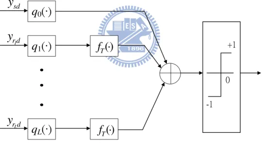
where ℜ{z} denotes the real part of z. Then the ML detector for BPSK signals is given by [24] ˆ x[n] = sgn [ q0(ysd[n]) + L ∑ i=1 fT (qk(yrd[n]); esrk) ] (2.5) where sgn[z] denotes the sign of the real number z and esrk is the ER of the link between

the source and the kth RN. (2.3) and (2.4.a)-(2.4.b) indicate that besides the instan-taneous received complex amplitude-to-noise-power ratio,

√ P_rkh_rkd[n] σ2 d and √ Pshsd[n] σ2 d , the hidden SR link’s ER, esrk, should also be known by the DN for ML detection. As the

instantaneous complex links gains hrkd[n] and hsd[n] are difficult to estimate in a high

require no such estimations. Nevertheless, [25] and [26] show that ML noncoherent de-tections of BFSK and DPSK signals by a DN still need the LT-CSI such as ERs for both far-end (SR) and near-end (SD and RD) links or σ2_d.

For notational brevity, we henceforth omit the subscript k associated with the kth relay, rk, unless there is danger of ambiguity. The DN of a single-relay BPSK-based

CCN has the samples {ysd[n], yrd[n]} of (2.1.a) and (2.2) as the sufficient statistics for

estimating the BERs of its component links. As an i.i.d. source is assumed, we can easily verify that the probability density function (pdf) of ysd[n] is independent of esr and so

is that of yrd[n]. With N coherently received sample pairs, {(q0(ysd[i]), q1(yrd[i]))} N i=1 △ = {(q(i) 0 , q (i)

1 )}, the joint conditional pdf f(ysd, yrd|Icsi) of the matched filter outputs, ysd

and yrd given CSI, {hsd, hrd, σd2, esr}= Icsi, and unit transmit powers, Ps = Pr = 1 is a

mixture density and the ML blind esr estimator is given by (see Appendix A.1)

ˆ

esr = arg max

0≤esr<0.5

log f ({ysd[i]}N_i=1,{yrd[i]}Ni=1|Icsi)

= arg max 0≤esr<0.5 N ∑ i=1 log [ cosh ( q(i)₀ + q(i)₁ 2 ) −2 sinh ( q(i)₀ 2 ) sinh ( q₁(i) 2 ) esr ] (2.6)

The reliability of the ML estimator depends on the sample size N , the true esr and

two other component links’ statistics which, in turn, determine those of q(i)₀ and q₁(i). For practical ERs, we usually need large N for the ML estimator to converge. The difficulty in implementing this estimator comes at least from three other concerns: (i) the computing complexity of solving the associated nonconvex optimization problem, (ii) there exists no recursive formula for updating the objective function whenever a new received signals pair becomes available, and (iii) the large required storage space. These implementation considerations convince us to turn to estimators based on the binary sample sequence {byrd[n],bysd[n]} produced by

byrd[n] = sgn [q1(yrd[n])] , bysd[n] = sgn [q0(ysd[n])] , (2.7)

easily extended to noncoherent binary modulations while the form of the ML estimator is highly modulation-dependent.

As a prelude to the study of simultaneous blind estimation of all component links’ ERs, we start with the simpler case of SR link ER estimation, assuming the ST-CSI needed and the ERs of either all or some of the remaining component links are available.

2.2

Side-Information-Aided Blind Single ER

Esti-mation

Since a cascaded link is composed of two (i.e. SR and RD) binary symmetric links (BSLs) with ERs, esrand erd, the end-to-end ER esrdis given by esrd = esr(1−erd)+(1−esr)erd= esr+ erd− 2esrerd. A single-relay CCN can thus be regarded as the composition of two

BSLs connecting the source and the destination. We assume stationary component links with time-invariant ERs and refer to the probability p = Pr(bysd =byrd) as the success

matching probability (SMP). Using the identity p = esdesrd+ (1− esd) (1− esrd) and the

i.i.d. source assumption, we immediately have following identity which relates various ERs to the SMP between a direct SD link and a cascaded SRD link

esr = 1− esd− erd+ 2esderd− p 1− 2esd− 2erd+ 4esderd

def

= esr(p) (2.8)

Since the links are assumed to be stationary, W [i]def= I (bysd[i] = byrd[i]), where I(E) = 1

if the statement E is true; otherwise it is zero, is Bernoulli distributed with success probability p. Furthermore, the SMP can be estimated by

bp(N ) ₌ N ∑ i=1 I (bysd[i] = byrd[i]) N , (2.9)

where the superscript (N ) indicates that N sample pairs are used to obtain the estimator. This average count based estimator is the sample mean of the Bernoulli process {W [i]} and is an uniform minimum variance unbiased estimator if i.i.d. samples are received [35].

Using the sample mean estimator (A.2) as ˆp, the method of moments and (2.8)

suggests the estimator besr =

1− esd− erd+ 2esderd− bp

1− 2esd− 2erd+ 4esderd = esr(ˆp) (2.10)

if both erd and esd are known. The derivations of (2.8) and (2.10) are given in Appendix

A.2.

As 0≤ esr ≤ 0.5, our estimator besr may have to be modified by the soft-limiter

J (besr) = min [max(besr, 0), 0.5] (2.11)

In addition, we can easily derive a recursive relation for bp(i) to sequentially estimate p and therefore esr.

The ER estimator (2.10) has many desired properties which we summarize in the following two lemmas.

Lemma 2.1. The estimator ˆesrdefined by (2.10) is (i) unbiased and attains the

Cramer-Rao lower bound (CRLB), (ii) an uniformly minimum variance unbiased (UMVU) and ML estimator with variance

Var(ˆesr) =

p(1− p)

N (1− 2esd− 2erd+ 4esderd)2

. (2.12)

where N is sample size.

Proof. See Appendix A.3.

Lemma 2.2. For any ε > 0, we have,

Pr(|besr− esr| ≥ ε) ≤ 2 exp

[ − min ( N2ε2C₁2 4p , N εC1 2 )] (2.13)

where C1 = 1− 2esd− 2erd+ 4esderd, N is sample size, and the soft-limiting effect (2.11)

is neglected.

The properties given in Lemma 2.1 are resulted from the fact that ˆesr is a linear

function of ˆp and the invariance property of an ML estimator. Lemma 2.2, which is

derived from using Chernoff’s inequality, implies that the estimator besr converges to esr

in probability.

2.3

Multiple-Relay-Aided Blind Multiple ER

Esti-mation

When there are L RNs, we have (L+1₂ ) combinatorial diversities from pairwise

hard-decision matchings. For any (k, l) RN pair, k ̸= l, the random variable, Wkl= I (byrkd =byrld),

is Bernoulli distributed with success (matching) probability pkl =Pr[byrkd = byrld] which

satisfies the identity

pkl= QkQl+ (1− Qk)(1− Ql) (2.14)

with Qk being the cascaded link ER given by

Qk = esrk + erkd− 2esrkerkd

def

= esrkd (2.15)

The above equations and (2.8) imply that psrk and pkl are related to the parameter sets

{esd, esrk, erkd} and {esrk, erkd, esrl, erld}, respectively. Following the approach used

for the case L = 1, we replace psrk and pkl in (2.8) and (2.14) by the average sample

count (sample mean) estimators

bpsrk = N ∑ j=1 I (bysd[j] =byrkd[j]) N , k = 1,· · · , L (2.16.a) bpkl = N ∑ i=1 I (byrkd[i] = byrld[i]) N , 1 ≤ k < l ≤ L (2.16.b)

to obtain(L+1₂ )equations, all of the form similar to (2.14), involving the unknown ERs,

{Qi} and esd.

When the RNs are dedicated stationary nodes and {er_kd} can be reliably estimated, there are only L+1 unknown parameters,{esd, esrk, k = 1,· · · , L}, which can be solved if

there are at least L + 1 independent equations. Since(L+1₂ )≥ L+1 whenever L ≥ 2, the unknown link parameters can be estimated as long as more than two RNs are available. For general multiple ER estimation in an L-relay CCN, L > 2, we can divide the problem into a sequence of subproblems, each deals with a smallest two-relay problem. For the detail, please refer to Table 2.1. The three-link (two relays plus a direct SD link) CCN is referred to as a basic network in which the link ER is governed by a set of nonlinear equations called a basic (nonlinear) system.

  11− Q− Q11− esd− Q2+ 2e+ 2Qsd1QQ21 1− esd− Q2+ 2esdQ2   =   ppsr121 psr2   ≈   bp_bpsr₁₂1 bpsr2   (2.17)

where bpsrl, l = 1, 2, and bp12 are obtained via (2.16.a) and (2.16.b). A similar nonlinear

system arose in [32] where the estimations of the error rates esd and Ql’s were attempted.

Unlike our case, there is no cascaded links and hence no need to estimate the ERs of the SR and RD links. It can be shown that the solution to the above basic system gives the basic estimators [36] (The derivation is given in Appendix A.5)

b Qi = 1 2− 1 2 √ (2bpij− 1)(2bpik− 1) 2bpjk − 1 , i, j, k∈ {0, 1, 2} (2.18) where bQ0 =besd, bp01 =bpsr1, and bp02= bpsr2.

The above equation indicate that the presence of multiple RD links enables us to estimate esd and removes the need for esd side information, i.e., the relay diversity can

be traded for the degree of LT-CSI. To estimate the ERs of the multiple hidden (far-end) SR links, we invoke the relation (2.15), assuming the ERs of all RD links are known, to obtain besrk = b Qk− erkd 1− 2er_kd , k = 1, 2. (2.19)

The flowchart of the proposed estimator is summarized in Table 2.1.

Note that an L-relay CCN induces(L+1₂ )basic systems (diversities) where each relay is involved in more than one system so that multiple estimates for a given Qi may be

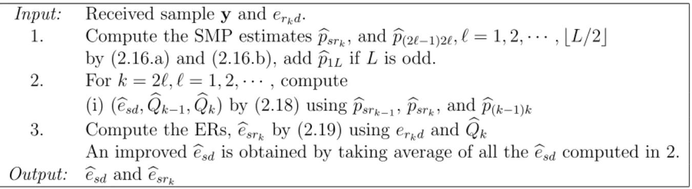
Table 2.1: A blind ER estimation algorithm for a multiple-relay CCN with knowledge of erkd.

Input: Received sample y and erkd.

1. Compute the SMP estimates bpsrk, and bp(2ℓ−1)2ℓ, ℓ = 1, 2,· · · , ⌊L/2⌋

by (2.16.a) and (2.16.b), add bp1L if L is odd. 2. For k = 2ℓ, ℓ = 1, 2,· · · , compute

(i) (besd, bQk−1, bQk) by (2.18) using bpsrk−1, bpsrk, and bp(k−1)k

3. Compute the ERs, besrk by (2.19) using erkd and bQk

An improved besd is obtained by taking average of all the besd computed in 2. Output: besd and besrk

obtained. Dixit [32] had proposed a complex method to take advantage of this fact and obtained improved ER estimates. On the other hand, [33] shows that the basic estimators given by (2.18) asymptotically achieve the accuracy achieved by the ML pilot-aided estimator based on the two sequences of hard-decision pairs, {bysd[i], byrld[i]}

N

i=1, l = 1, 2,

for finite N , a better estimate is obtained by maximizing the log-likelihood functions, Γ({bysd[i],byrld[i]})

def

= log f ({bysd[i],byrld[i]}

N

i=1), l = 1, 2, defined as

Γ({bysd[i],byrld[i]})

= N ∏ i=1 ( e1−I(bysd[i]=x[i]) sd (1− esd) I(bysd[i]=x[i]) 2 ∏ l=1

Q1_l−I(byrld[i]=x[i])(1− Ql)I(byrld[i]=x[i])

)

The derivation of the above function is similar to that given in [33, Section III] with additional consideration of cascaded link ER Ql. In [33] an EM based approach was

proposed to obtain blind (unknown x[i]) estimates of Qi which outperforms Dixit’s

method. However, our numerical experiments conclude that, for both approaches, the

performance improvement over the basic estimators is rather limited and do not worth the additional high complexity; see Section VI and Fig. 4.4.

Before presenting our main results in the following sections, we would like to em-phasize that most estimators to be developed are based on some variation or extension of the basic system (2.17) and their expressions, e.g., (3.5.a)-(3.6), (3.9.a)-(3.9.d), and

(3.11.a)-(3.12.b), are derivable from variations or extensions of the basic estimators, (2.18) and (2.19).

Chapter 3

Blind Multiple ERs Estimation

using Virtual Links

We first examine the ER ambiguity issue associated with the estimation of a far-end component link’s ER and then present a novel solution to resolve this ambiguity. The extension to other binary modulations–BFSK and DPSK–is discussed at the end of this chapter.

3.1

ER ambiguity in a cascaded link

As can be seen from (2.17), when there are sufficient relays, the resulting equation set leads to formulae for the estimates of esd and Qk but not those for esrk and erkd. This

is due to the fact that the ER of an SRD link, as (2.15) has shown, is a symmetric function of the ERs of the associated component SR and RD links, i.e., there are infinite many (esrk, erkd) pairs that result in the same Qk. In fact, the legitimate candidates

for the latter two ERs consist of the lower-left part of the hyperbola defined by (2.15), (1− 2Qk)/4 = (esrk −

1

2)(erkd−

1

2), that lies within the square S

def = {(esr_k, erkd)|0 < esrk < 1 2, 0 < erkd < 1

2}. The ambiguity in (2.15) is resolved in the scenario discussed in the last section by specifying erkd so that besrk is obtained via (2.19) (see Fig. 3.1).

Geometrically, this is equivalent to finding the intersection of the hyperbola and the line

erkd= e within the square S, where e is the true ER of the RD link.

˦̂˿̈̇˼̂́

sd

e

rd

e

rd

e

e

Q

Figure 3.1: Ambiguity problem can be solved if the knowledge erd= e is available.

another set of legitimate ER pairs and which has only one intersection point with (2.15) in S. Since the hyperbola is symmetric with respect to the line er_kd = esrk and we

have access to the outputs of the RD and SD links only, finding a curve which has a unique intersection with (2.15) is possible if an alternate RD link is provided. This can be seen by noting that a RD link with a different average bit SNR γ yields a different equivalent cascaded link with ER Q′_k and therefore a curve of the form (1− 2Q′_k)/4 = (esrk−

1

2)(αerkd−

1

2), where α is such that 0 < αerkd

△

= er′_kd< 1₂.

3.2

Virtual link methods

To have an alternate physical link (PL), one can purposely vary the power of the bit stream so that the transmitted sequence is equivalent to one formed by multiplexing two

data sources with different powers. If the locations of these two parts in the multiplexed data stream are known, the DN then perform separate comparison and counting based on (2.16.a) and (2.16.b). Although such a two-level amplitude modulation makes pos-sible solving the esrk, erkd ambiguity, allocating unequal powers to different parts of the

transmitted data stream is often undesirable. This dilemma can be avoided by creating a virtual link (VL) without modifying the existing link.

A VL can be created by rotating the received I-Q vector counter-clockwise by an angle θ between 0o_{and 90}o_{. This is equivalent to introducing an artificial phase offset to}

the received samples which are then used as outputs from another link. Since the noise is circular symmetric, the rotation results in an equivalent signal power degradation cos2θ

without altering the noise statistic. Such a virtual SNR loss cannot be accomplished by simply multiplying the BPSK matched filter output by a positive constant less than one.

An alternate method is to add an extra zero-mean white Gaussian noise component to the received in-phase samples. Both schemes give a VL with a smaller γ. The second scheme–the addition of a perturbation term–incurs no hardware increase but requires the estimation of noise power σ_d2, which is needed in subsequent ML detection anyway. As the phase-rotation scheme leads to an SNR degradation of magnitude cos2θ, the

second scheme has to generate i.i.d. zero-mean Gaussian random samples with variance

σ2

v = σ2d(1/ cos2θ− 1) to achieve the same SNR loss. Although both approaches achieve

the same effect for BPSK signals, the phase-rotating approach cannot produce a VL for noncoherent systems while the method of inserting extra noise suits both coherent and noncoherent applications. Hence, except for the coherent system discussed in this section, we will adopt the noise-injection approach in the following sections.

We use the superscript (v) to indicate that a parameter is associated with a VL, i.e., the kth RD link’s synchronous output samples and their rotated (VL) versions are denoted by yrkd[n], y

(v)

rkd[n] and the corresponding ERs by erkdand e

(v)

system operating in a flat Rayleigh fading environment, we have [37] P_bpsk(γ) = 1 2 ( 1− √ γ 1 + γ ) , (3.1) which is equivalent to γ = (1− 2P psk b ) 2 1− (1 − 2P_bpsk)2. (3.2)

The two ERs are then related by (1− 2er_kd)2 1− (1 − 2er_kd)2 = 1 cos2_θ (1− 2e(v)_r kd) 2 1− (1 − 2e(v)_r kd) 2. (3.3)

Following a procedure similar to that for solving (2.17), we can easily show that the nonlinear system which consists of (2.15), (3.3) and the new cascaded link’s ER equation

Q(v)_k = esrk+ e

(v)

rkd− 2esrke

(v)

rkd (3.4)

has the closed-form solution

esrk = 1−√1− 4t 2 , erkd= Qk− esrk 1− 2esr_k, (3.5.a) e(v)_r kd = Q(v)_k − esr_k 1− 2esr_k . (3.5.b) where t = (1− 2Q (v) k ) 2_Q k(1− Qk) (1− 2Q(v)_k )2− cos2_θ(1− 2Qk₎2 − cos2θ(1− 2Qk)2Q(v)_k (1− Q(v)_k ) (1− 2Q(v)_k )2− cos2_θ(1− 2Qk₎2. (3.6) Based on this solution, we can obtain a complete blind algorithm to estimate the ERs of all component links by using the estimates for Qk and Q

(v)

k which are computed

via (2.18) using another, say lth (l ̸= k) relay link; ER side information is no longer needed. In short, to estimate the triplet (esd, esrk, erkd) associated with an SD and an

SRD links without the help of CSI, one needs another independent relay. The auxiliary relay requirement can be waived if one creates a virtual SD link to obtain additional combinational diversities. In general, the rotation angle for producing a virtual SD link can be different from that for a virtual RD link. However, we lose no generality by

assuming both rotation angles are the same, say θ. Denote bybp(vs)r,bps(vr)and bp(vs)(vr)the estimates for the SMPs, Pr(by

(v) sd =byrd), Pr(bysd =by (v) rd), and Pr(by (v) sd =by (v) rd), respectively,

and by Q = esrd, Q(v) = es(vr)d, the ERs for the SRD and the SR-plus-virtual relay links.

We obtain four nonlinear relations for a single-relay CCN:

bpsr = esdQ + (1− esd)(1− Q) (3.7.a) bp(vs)r = e (v) sd Q + (1− e (v) sd)(1− Q) (3.7.b) bps(vr) = esdQ(v)+ (1− esd)(1− Q(v)) (3.7.c) bp(vs)(vr) = e (v) sd Q (v) + (1− e(v)_sd)(1− Q(v)) (3.7.d) With the additional PL-VL relation

(1− 2esd)2 1− (1 − 2esd)2 = 1 cos2_θ (1− 2e(v)_sd )2 1− (1 − 2e(v)_sd)2 (3.8)

the nonlinear system (3.7.a)–(3.8) yields the closed-form estimators besd = 1 2 [ 1− bpsr− bQ 1− 2 bQ + 1− bps(rv)− bQ(v) 1− 2 bQ(v) ] (3.9.a) b Q =1− √ 1− 4t1 2 , Qb (v) = 1− √ 1− 4t2 2 (3.9.b) t1 = cos2_θ(2bp sr− 1)2(bp(vs)r− 1)bp(vs)r (2bp(vs)r− 1)2− cos2θ(2bpsr− 1)2 − (2bp(vs)r− 1)2(bpsr− 1)bpsr (2bp(vs)r− 1)2− cos2θ(2bpsr− 1)2 (3.9.c) t2 = cos2_θ(2bp s(vr)− 1)2(bp(vs)(vr)− 1)bp(vs)(vr) (2bp(vs)(vr)− 1)2− cos2θ(2bps(vr)− 1)2 − (2bp(vs)(vr)− 1)2(bps(vr)− 1)bps(vr) (2bp(vs)(vr)− 1)2− cos2θ(2bps(vr)− 1)2 . (3.9.d) Estimators,besrandberd, can be derived from solving the nonlinear system which includes

(2.15), (3.3) and an equation similar to (3.4). An analytic solution of this nonlinear system is obtained by substituting (3.9.b) into (3.6) and then (3.5.a). As has been men-tioned in Section I, we refer to ER estimation algorithms using the approach described in this section as virtual link aided (VLA) estimators. The corresponding estimation procedure is included in Table 3.1.

Note that the SMP formulae (2.14) and (3.7.a)-(3.7.d) are not valid for the SMP between a PL and its virtual version since their outputs are correlated. Actually, this

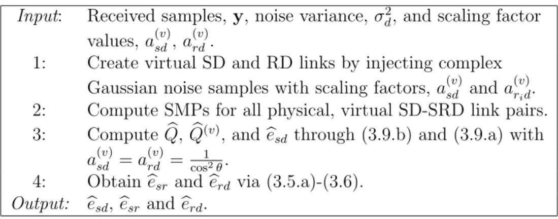
Table 3.1: A blind ER estimation algorithm for BPSK modulation.

Input: Received samples, y, noise variance, σ2

d, and scaling factor

values, a(v)_sd, a(v)_rd.

1: Create virtual SD and RD links by injecting complex Gaussian noise samples with scaling factors, a(v)_sd and a(v)_r

id.

2: Compute SMPs for all physical, virtual SD-SRD link pairs. 3: Compute bQ, bQ(v)_{, andbe}

sd through (3.9.b) and (3.9.a) with a(v)_sd = a(v)_rd = _cos12_θ.

4: Obtainbesr and berd via (3.5.a)-(3.6). Output: besd, besr and berd.

SMP is the sum of two conditional SMPs defined by (4.28) and (4.29) which are derived in Appendix D. Obviously, a system involves these two nonlinear expressions does not easily render a closed-form solution. On the other hand, a VL can provide a new SMP relation similar to (2.14) with each different PL or its virtual version and a single-relay CCN can offer two uncorrelated VLs to render a basic system that consists of three independent SMP equations, we thus conclude that, by using both virtual RD and SD links, one can estimate all ERs of a single-relay CCN without side information.

3.3

Blind ER Estimation for BFSK and DPSK

Sig-nals

Although we have limited our discussion to BPSK signals so far, such a restriction does not lose any generality as far as the VL concept is concerned. The proposed blind estimation method in the last section can easily be extended to noncoherent binary modulations because our estimation scheme can be applied for any binary symmetric channel. Besides using (noncooperative) noncoherent detectors, the DN adds a complex Gaussian perturbation term to each of the received noncoherent sample to generate the corresponding VL with the desired equivalent average SNR.

decisions. Since, for the noncoherent case, the definition and estimation of SMPs are the same as those of the BPSK-based system, we have four nonlinear equations similar to (3.7.a)–(3.7.d) which relate the SMPs to the corresponding ERs of the connecting SD and cascaded SRD links. The relation between the ER of a cascaded link and its two component links remains the same we thus obtain two equations similar to (2.15) and (3.4). However, as different modulation type is involved, the equation governing the relation between esd’s for the physical and the virtual links is different from (3.3), so is

that between the two erd’s. The new relation can be expressed in the generic form

Fe(z) = a(v)Fe(z(v)), (3.10)

where z = esd or erd and, as before, the superscript (v) on the right-hand side denotes

the corresponding set of parameters for the VL. (3.10) is similar to (3.3) but the actual expression for Fe(z) depends on the modulation used and a(v) is a scaling parameter

related to the variance of the injected noise (normalized with respect to σ2

d).

Solving the nonlinear system consisting of the SMP equations and Fe(esd) = a(v)Fe(e

(v) sd ), we obtain b Q =(1− 2bpsr) [ 1− bp(vs)r ] − a(v)[₁− 2bp (vs)r ] (1− 2bpsr) (1− 2bpsr)− a(v) [ 1− 2bp(vs)r ] (3.11.a) b Q(v)= [ 1− 2bps(vr) ] [ 1− bp(vs)(vr) ] [ 1− 2bps(vr) ] − a(v)[₁− 2bp (vs)(vr) ] − a(v) [ 1− 2bp(vs)(vr) ] [ 1− 2bps(vr) ] [ 1− 2bps(vr) ] − a(v)[₁− 2bp (vs)(vr) ] (3.11.b) besd = 1 2 [ 1− bpsr− bQ 1− 2 bQ + 1− bps(vr)− bQ(v) 1− 2 bQ(v) ] (3.11.c) Similarly, we have besr = b Q(v)− 2 bQ bQ(v)− a(v)Q + 2ab (v)Q bbQ(v) 1− 2 bQ− a(v)_{+ 2a}(v)_Qb(v) (3.12.a) berd = b Q− besr 1− 2besr . (3.12.b)

The explicit forms of Fe(z) for different modulations and the corresponding relations

used for computing the ER estimators are listed in Table 3.2. The estimation procedure is summarized in Table 3.3.

Table 3.2: The required CSI and the solutions of nonlinear systems under various mod-ulations.

Fe(x) Q Q(v) esd esr erd

BPSK _1−(1−2x)(1−2x)22 (3.9.b) (3.9.b) (3.9.a) (3.5.a) (3.5.a)

BFSK 1−2x_x (3.11.a) (3.11.b) (3.11.c) (3.12.a) (3.12.b) DPSK 1−2x_2x (3.11.a) (3.11.b) (3.11.c) (3.12.a) (3.12.b)

Table 3.3: A blind ER estimation algorithm for BFSK/DPSK modulation.

Input: Received samples, y, noise variance, σ2_d, and scaling factor values, a(v)_sd, a(v)_rd.

1: Create virtual SD and RD links by injecting complex Gaussian noise samples with scaling factors, a(v)_sd and a(v)_r

id.

2: Compute SMPs for all physical, virtual SD-SRD link pairs. 3: Compute bQ, bQ(v), andbesd by using (3.11.a)-(3.11.c).

4: Obtainbesr and berd based on (3.12.a) and (3.12.b). Output: besd, besr and berd.

3.4

Simulation Results

For convenience of reference we refer to the ML detector using the ER estimators pre-sented in Section II as the physical-link-only (PLO) detector and that using a VLA estimator as the VLA detector. The ML detector with perfect CSI is called the ideal detector. Let dsrk, drkd, dsd be the distances of the kth SR, RD links and the SD link

and θsrk be the angle between the SD and kth RD links; see Fig. 1.2. Without loss of

generality, we use the normalization, dsd = 10 so that d2_srk = d2_rkd+ d2_sd− 2dr_kddsdcos θsrk = 100 + d

2

rkd− 20drkdcos θsrk, (3.13)

We assume the path loss model, σ2

ij ∝ d−αij with the normalization σ2sd = 1 and α > 0.

Denote by σ2

ij the variance of the Rayleigh faded link gain and dij the distance between

node i and node j, (i, j) ∈ {(s, rk), (rk, d), k = 1,· · · , L}. All the simulated performance

curves are obtained by sequentially applying the proposed methods, i.e., the estimated ERs are updated sequentially as each new sample becomes available and the updated

estimates are then used for detecting each received bit. As in [25], we define the SH average SNR as the average received SNR for the direct SD link without relaying, ¯γsd.

Simulation for a given ¯γsdterminates whenever the number of error events in the detector output exceeds 500. We assume that noise powers at DN and RN are the same, σ2

d = σr2,

and use the normalization P = Ps+

∑L

i=1Pri = 1 such that ¯γsd = 1/σ

2

d. To reduce the

complexity of the ML detector, [24] suggested a piecewise linear function to approximate the nonlinearity (2.3). As it causes negligible performance degradation with respect to that of the ML detector so long as esrk <

1

2, we use the same approximation in our simulation efforts. Fig. 3.2 illustrates the block diagram of the maximum likelihood (ML) detector, where fT(t) is approximated by a piecewise linear function: fT(t; esrk)≈

min(max(t,−T ), T ) and T = ln (_1−e srk e_srk ) .

q

ʻ ʼ

q

ʻ ʼ

q

ʻ ʼ

y

y

)

(˜

f

)

(˜

f

y

Figure 3.2: Block diagram of the maximum likelihood (ML) detector.

The performance of the PLO and VLA detectors for the simplest case, L = 1 with BPSK modulation, is illustrated in Fig. 3.3. For the PLO detector, only esr is unknown

while the VLA detector assumes ERs of other component links are also unavailable and uses a rotation angle θ = 45◦, which is equivalent to injecting noise with a(v)_sd = a(v)_rd = 2. The performance of both detectors are found to approach that of the ideal ML detector.