利用高解析度彩色影像提升時差測距深度圖的品質

國

立

交

通

大

學

電子工程學系 電子研究所

碩 士 論 文

利用高解析度彩色影像提升時差測距深度圖的品質

TOF-Sensor Captured Depth Map Refinement

Using High-Resolution Color Images

研 究 生：陳敬昆

指導教授：杭學鳴教授

利用高解析度彩色影像提升時差測距深度圖的品質

TOF-Sensor Captured Depth Map Refinement

Using High-Resolution Color Images

研 究 生: 陳敬昆 Student: Ching-Kun Chen

指導教授: 杭學鳴 教授 Advisor: Prof. Hsueh-Ming Hang

國 立 交 通 大 學

電子工程學系 電子研究所碩士班

碩 士 論 文

A Thesis

Submitted to Department of Electronics Engineering and Institute of Electronics

College of Electrical and Computer Engineering National Chiao Tung University

In Partial Fulfillment of the Requirements for the Degree of

Master of Science in

Electronics Engineering

July 2014

Hsinchu, Taiwan, Republic of China

i

利用高解析度彩色影像提升時差測距深度圖的品質

研究生 : 陳敬昆 指導教授 : 杭學鳴 教授

國立交通大學

電子工程學系 電子研究所碩士班

摘要

隨著人機互動(Human-Machine Interaction)的發展，人們可以更直覺地操作電腦。 Microsoft 在 2010 年發表的 Kinect for Xbox 360 可以視為人機互動發展的里程碑。玩家 不需要任何穿戴裝置，就可藉由簡單的肢體動作對 Xbox 360 下達指令。而人們可以有 如此豐富的遊戲體驗都要歸功於 Kinect。Kinect 是一台深度攝影機，它會依照距離偵測 前方物體的深度值並轉譯成深度圖。雖然 Kinect 深度圖的解析度非常小，卻是 Xbox 360 辨識人體動作的重要資訊來源。深度圖的品質對於電腦識別的結果有很大的影響，所以 如何提升深度圖的解析度已經成為一個重要議題。

在本實驗中，我們使用 MESA Imaging 在 2008 年生產的時差測距(Time-of-Flight)深 度攝影機 SR4000 來擷取深度資訊。然而 SR4000 的解析度只有 176×144，如此低的解析 度會限制許多深度圖應用的發展，因此我們使用一台超高解析度彩色攝影機 Flea3 把 SR4000 的解析度提升到跟彩色攝影機一樣高。Flea3 是 Point Grey 在 2012 年生產的超 高解析度彩色攝影機，它最高的解析度可以達到 4096×2160。

我們提出一個「深度精煉演算法」，它可以藉由高解析度彩色照片來提升深度圖的

ii 又模糊的深度圖轉變成高解析度深度圖。深度精煉演算法可以藉由參考彩色影像來得知 正確的物體邊界，進而正確地修正深度圖。因為這個演算法只適用於小範圍的影像，所 以深度圖與彩色影像會被各別拆解成好幾個小塊再做處理。最後我們拿我們提出的高解 析度深度圖與傳統內插法產生的深度圖相比，實驗結果顯示，深度精煉演算法可以產生 更自然的高解析度深度圖。

iii

TOF-Sensor Captured Depth Map Refinement

Using High-Resolution Color Images

Student: Ching-Kun Chen Advisor: Prof. Hsueh-Ming Hang

Department of Electrical Engineering &

Institute of Electronics

National Chiao Tung University

Abstract

Kinect for Xbox 360 made by Microsoft Company in 2010 is a milestone for

Human-Machine Interaction (HMI). Without any sensor wearing on body, players can send commands to Xbox 360 directly by simple limb motion. Kinect has a depth camera for producing depth maps as object descriptor. Its depth map has a rather low resolution and for many other applications, we need high quality depth maps. Hence, how to improve the resolution of depth maps has become a major research topic.

In our experiments, we use a Time-of-Flight (ToF) camera (SR4000) to get the depth information. However, the resolution of SR4000 is only 176×144 pixels. We thus use a high resolution color camera to collocate with SR4000, and we wish to improve the depth map resolution based on the high resolution color images. Flea3 is used in our experiments which is produced by Point Grey Company in 2012. Its maximum resolution is 4096×2160.

We propose a depth refinement algorithm to enhance the low resolution depth maps using high resolution color images. Align depth maps and color images at the same view point,

iv

the depth refinement algorithm can transform the small and blurred depth map into high resolution one. Based on the color images, our depth refinement algorithm can extract the exact object edges and revise the depth maps correctly. Because this algorithm is suitable for small, local regions, the depth maps and color images are divided into several patches and are processed individually. Finally, we compare the interpolated depth maps with the proposed high resolution depth maps. Experimental results show that our depth refinement algorithm can produce a good quality, high resolution depth map.

v

誌謝

在我碩班生涯裡，最要感謝杭學鳴老師。是杭老師給了我人生的轉捩點，老師給我 的機會還有恩情，真的太多了，如果不是老師願意收留，我不可能有現在的碩士學位， 也不會有機會認識 commlab 這些朋友。我很感激老師願意讓我待在他身邊偷學，學研究、 學態度，也學做人。在與自己知識差距懸殊的學生面前，老師依然掛著謙虛的微笑，然 後輕鬆的指出報告中的盲點，真的太神啦！好希望有一天可以達到老師這種又強又謙虛 的境界。對老師的感激，真的不可能寫完，我會永遠記在心裡等機會報答的。 接下來要感謝整個杭 group。感謝馬哥幫我磨練嘴砲技能，能夠抵擋這麼猛烈的砲 火還絲毫未損的強者真的不多。感謝鈞凱借我好多參考資料，從碩論、作業到履歷表， 讓我省很多摸索的功夫。感謝長廷、鬢角周末回來陪嘴砲，壓力減輕不少。感謝大摳陪 我吃宵夜聊天，根本人生導師。感謝司頻在口試幫我做很多雜事，各種貼心。感謝育綸、 欣哲讓我問很多口試流程的問題。感謝靖倫陪我準備口試。感謝治戎、小哲瑋、Amanda， lab 接下來就靠你們了。 然後要感謝整個 commlab 溫馨大家庭。感謝威哥整天跟我聊一些有的沒的，每次緊 張的事聊完都不緊張了。感謝小本、拔剌、昀楷、阿郎、佳佑、阿楚、駝獸、柏佾、棒 賽，地球有你們真好，守護世界和平就交給你們了。雖然我覺得…沒差。呵呵~ 最後要感謝我老爸、老媽、老姊、叔叔、阿公跟阿罵。謝謝你們耐著性子拉拔我長 大，忍受這個任性難管教又三不五時惹麻煩的兒子。辛苦你們了。接下來，就交給我吧。 媽！我在這！！ 妳兒子畢業了啦！！！ 有厲害齁~ 哈哈哈哈哈…哈哈哈哈哈… XDDDD 陳敬昆 一○三年七月於 風城 交大 謹致

vi

Contents

摘要 ... i Abstract ... iii 誌謝 ... v Contents ... vi

List of Figures ... viii

Chapter 1. Introduction ... 1

1.1 Background ... 1

1.2 Motivations and Contributions ... 2

1.3 Organization of Thesis ... 2

Chapter 2. Depth Map ... 3

2.1 Depth Map from Structured Light Camera ... 6

2.2 Depth Map from Time-of-Flight (ToF) Camera ... 10

2.3 High Resolution Depth Map ... 14

Chapter 3. Experiment Environment and Image Calibration ... 18

3.1 Experiment Devices and Setup ... 18

3.1.1 The Depth Camera ... 18

3.1.2 The Color Camera ... 20

3.1.3 Experiment Setup ... 21

3.2 Depth and Color Images Calibration ... 22

3.2.1 Camera Distortion Calibration ... 22

3.2.2 Alignment of Depth and Color Images ... 25

Chapter 4. Depth Map Refinement Algorithm ... 29

4.1 Overview of the Proposed Method ... 29

4.2 Patches ... 30

4.3 Color Images Clustering ... 31

4.3.1 Median Filter ... 32

4.3.2 L*a*b* Color Space ... 33

4.3.3 Segmentation and K-means Clustering ... 39

4.4 Depth Map Clustering ... 43

4.4.1 Spreading ... 43

4.4.2 Classification ... 45

4.4.3 Statistics ... 46

4.4.4 Correction ... 48

4.5 Depth Pixels Interpolation ... 51

4.5.1 Separation ... 52

4.5.2 Expansion ... 53

vii

4.5.4 Combination ... 55

4.6 Experimental Results ... 56

Chapter 5. Conclusions and Future Work ... 60

5.1 Conclusions ... 60

5.2 Future Work ... 60

viii

List of Figures

Figure 1. Dataset captured by the Kinect sensor [1]... 4

Figure 2. Rendered 3-D scene results based on two depth maps [1]... 4

Figure 3. 3DV data: Newspaper [2] ... 5

Figure 4. Kinect™ for Xbox 360® [3]... 6

Figure 5. The experimental results of [4] ... 8

Figure 6. The experimental results of [5] ... 9

Figure 7. Kinect™ for Xbox One® [6] ... 10

Figure 8. PMD[vision]® CamCube 3.0 [7] ... 10

Figure 9. Edge detection result of [8] ... 12

Figure 10. Denoised depth maps in [8] ... 13

Figure 11. Setup containing Kinect for Xbox 360 and SR4000 [10] ... 14

Figure 12. The experimental result of [9] ... 15

Figure 13. The experiment setup and result of [11] ... 16

Figure 14. The experiment setup and result of [12] ... 17

Figure 15. MESA Imaging SR4000 - ToF Depth Camera [13] ... 18

Figure 16. Images captured by the color and depth camera. ... 19

Figure 17. Point Grey Flea3 USB 3.0 - Color Camera [15] ... 20

Figure 18. Theia Technologies MY110M - Ultra Wide Lens [16] ... 20

Figure 19. The experiment setup ... 21

Figure 20. Depth and intensity maps before and after camera distortion calibration ... 23

Figure 21. Checkerboard images for Camera Calibration Toolbox ... 24

Figure 22. Alpha blending of the resized depth and color images... 26

Figure 23. Alignment Algorithm ... 27

Figure 24. Alignment result of the depth map ... 28

Figure 25. The flow diagram of the depth refinement algorithm ... 29

Figure 26. Patches of the color image ... 30

Figure 27. Result of the median filter ... 32

Figure 28. Edge Classification [18] ... 33

Figure 29. ROC curves for each channel in each color space [18] ... 34

Figure 30. sRGB in L*a*b* color space [19] ... 36

Figure 31. Remove the L* axis from the L*a*b* color space ... 37

Figure 32. Unify the intensity of L* ... 38

Figure 33. The image matting result using [20] ... 39

Figure 34. The image matting result using [20] ... 40

Figure 35. The k-means clustering result ... 42

Figure 36. The k-means clustering result with the median filter ... 42

ix

Figure 38. Illustration of sparse depth pixels overlapped with the color image ... 45

Figure 39. The down-sampling classification result of the color image ... 46

Figure 40. The histogram of depth pixels ... 47

Figure 41. The corrected result of the depth map ... 49

Figure 42. The corrected result of the sparse depth map overlapped with the color image ... 50

Figure 43. Separation of the depth map ... 52

Figure 44. Dilation of each class ... 53

Figure 45. Reshape the blurred edge ... 54

Figure 46. The result of combination ... 55

Figure 47. The experimental results ... 57

Figure 48. The experimental results ... 58

1

Chapter 1. Introduction

1.1 Background

The Human-Machine Interaction (HMI) techniques advance quickly in the past two decades. One step beyond touch control, Kinect for Xbox 360 by Microsoft Company in 2010 [3] is pioneering in motion control in consumer market. However, the depth maps produced by Kinect suffer serious occlusion problem and are too rough to detect tiny movement of human body such as fingers. Thus, research on filling up occlusion regions and broken holes on Kinect depth maps becomes popular [4] [5].

Kinect for Xbox 360 in 2010 used a structured light camera. The structured light camera has the advantage of large scanning area and low-cost hardware, but its depth maps are sketchy and suffer from severe occlusion problem. Thus, the other type of depth sensor, the Time-of-Flight (ToF) camera, becomes popular [6]. Although the hardware of ToF camera costs more, the depth maps captured by ToF camera are more accurate and contain less occlusion regions. The new Kinect for Xbox One released by Microsoft Company in 2014 also uses the ToF camera.

Occlusion problem can be resolved by changing hardware, but the problem about low resolution is not. The resolution of new Kinect for Xbox One is 640×480. Although the resolution is twice that of Kinect for Xbox 360, it is not enough to some applications. Thanks to mature technology of digital camera, the high resolution and low cost color images can offer a feasible solution. Using the high resolution color images to compensate for the low resolution depth maps is an economical method. Nowadays, research on combining color images and depth maps is fast growing [9] [11] [12].

2

1.2 Motivations and Contributions

The low resolution of depth maps is a troublesome problem and has no low-hardware solution in the present day. Many applications need high-quality depth maps, such as virtual view synthesis, object recognition, and depth image based rendering (DIBR). However, the development of these applications is restricted because of the low resolution of depth maps. If we can improve the quality of depth maps efficiently, it is helpful to the 3D products, such as Free Viewpoint Television (FTV), Kinect or other Human–Machine Interaction (HMI) devices.

In this thesis, we propose a depth refinement algorithm to increase the resolution and quality of depth maps. Experimental results show that the proposed scheme indeed produces high resolution depth maps. There is no large occlusion region like Kinect for Xbox 360 or many artifacts are significantly reduced.

1.3 Organization of Thesis

We first describe the characteristics of depth maps using different depth cameras. We also introduce some previous research works on enhancing depth map in chapter 2. The experiment environment, device setup and image calibration between depth maps and color images are discussed in chapter 3. Then, chapter 4 describes our proposed depth map refinement algorithm; this is main theme of this thesis. Finally, we conclude this thesis with some future work in chapter 5.

3

Chapter 2. Depth Map

The depth map is a very important component in 3D image applications. Many 3D image processing techniques rely on depth maps, such as virtual view synthesis, object recognition, and depth image based rendering (DIBR). The quality of depth maps has significant impact on the result of 3D image processing We take image rendering as an example. Figure 1(a) and (b) are the dataset captured by the Microsoft Kinect sensor in [1]. The raw depth map of the Kinect sensor in Figure 1(b) is broken and lacks details. In [1], the raw depth map is enhanced with alpha channel estimation and the enhanced result is shown in Figure 1(c). Obviously, the enhanced depth map in Figure 1(c) is better in quality than the raw depth map in Figure 1(b). The rendering results of the raw and the enhanced depth map are shown in Figure 2. Because the edge of objects in raw depth map is too broken, the rendering result is factitious and contains artificial holes, as in Figure 2(a). In contrast, the rendering result of the enhanced depth map shown in Figure 2(b) has better visual quality. Therefore, the quality of depth maps is an important subject of 3D research and the depth map refinement algorithm is our focus in this thesis.

There are many 3D video test sequences provided by researchers. Figure 3(a) and (b) are the 3DV dataset named Newspaper and produced by Gwangju Institute of Science and Technology (GIST) [2]. However, the depth map in Figure 3(b) is not captured by a depth camera. Because depth cameras nowadays cannot provide depth maps with a resolution as high as the color images, we have to spend a lot of time manually produce depth maps using software. The produced high resolution depth map is not all precise. Figure 3(c) is an alpha blending of Figure 3(a) and (b). In Figure 3(c), the edge of the color image and the depth map do not match well. The quality of depth maps from the test sequences need to be improved.

4

(a) Color image (b) Raw depth map

(c) Various enhanced depth maps

Figure 1. Dataset captured by the Kinect sensor [1]

(a) Raw depth map (b) Enhanced depth map

5

In chapter 2, we introduce depth maps captured by two types of commonly used depth cameras, structured light camera and time-of-flight (ToF) camera. A popular model the structured light camera is Kinect for Xbox 360 announced by Microsoft Company in 2010, as shown in Figure 4. The second type ToF camera is used in our experiment, which is SR4000 produced by MESA Imaging Company in 2008 and shown in Figure 15.

After introducing the depth maps captured from depth cameras, we will describe some high resolution depth map algorithms proposed by the previous researchers and compare their experimental results with ours.

(a) The color image (b) The depth map

(c) Alpha blending of (a) and (b)

6

2.1 Depth Map from Structured Light Camera

The structured light camera is a widely used depth camera because of its large scanning area, short scanning time and low-cost hardware. One of the well-known structured light cameras is Kinect for Xbox 360 developed by Microsoft Company in 2010, as shown in Figure 4. The technique Kinect uses to get depth information is “Light Coding” developed by PrimeSense Company. Light Coding uses an infrared emitter to encode the whole measured space, and a receiver decodes the reflected infrared to produce a depth map. The principle of Light Coding is “Laser Speckle”. When the laser light illuminates the surface of objects, the reflected light forms many kinds of speckles. The speckle pattern is semi-random and changes with distance. Any two patterns in the measure space are different, so it acts like the entire space is marked. The Light Coding technique can decode these laser speckles to compute the depth information and transform it into depth maps.

The image resolution of Kinect is very low compared with the digital cameras nowadays. The resolution of its own color camera is 640×480 and the depth camera is 320×240. Due to its high noise, the produced depth map cannot show tiny objects. In Figure 5(f), the fingers cannot differentiate clearly. In addition to low resolution and high noise, Kinect suffers from severe occlusion problem. Because the emitter and receiver of the depth camera are not in the same position, the background objects which can be illuminated by the emitter may be occluded by the foreground objects and cannot be seen from the viewpoint of the receiver. The reflected light of background objects cannot be captured by the receiver, so

7

their depth maps have no depth information in this region. The region without depth

information is shown as pure black or white, and it is the so-called occlusion region. In Figure 5(d), there is a pure white and overlapped shadow of fingers. In Figure 6(d), there is a pure black and duplicated hole of palms. Both of them are occlusion region.

Researchers on how to fill up occlusion region is popular. In [4] and [5], they proposed a spatial and temporal method respectively to deal with occlusion problem. Figure 5(g), (h) and (i) are enhanced depth maps of [4]. Although the occlusion region is filled, the edge of depth maps cannot match color images completely. Because the resolution of color images is only twice the resolution of depth maps, the color images cannot provide detailed information of objects to increase the accuracy of depth maps dramatically. Figure 5(j), (k) and (l) use alpha blending of color images and enhanced depth maps to show the quality improvement of depth maps. There are still visible artifacts. Similarly, Figure 6(g), (h) and (i) are enhanced depth maps of [5]. It cannot sharpen the edge of depth maps either.

8

(a) (b) (c) Color images

(d) (e) (f) Raw depth maps of Kinect (g) (h) (i) Enhanced depth maps

(j) (k) (l) Alpha blending of color images and enhanced depth maps

9

(a) (b) (c) Color images of a sequence (d) (e) (f) Raw depth maps of Kinect (g) (h) (i) Enhanced depth maps

10

2.2 Depth Map from Time-of-Flight (ToF) Camera

Time-of-flight (ToF) camera is another popular type of depth camera with short scanning time and simple algorithm. The resolution of ToF camera is influenced by ambient light. Compared with structured light camera, ToF camera has more accurate depth maps but higher-cost hardware. Kinect for Xbox One by Microsoft Company in 2014 shown in Figure 7, PMD[vision] CamCube 3.0 by pmdtechnologies Company in 2009 shown in Figure 8 and SR4000 by MESA Imaging in 2008 shown in Figure 15 are a few ToF cameras in the market. The depth camera we used in our experiments is SR4000. The principle and specification of SR4000 will be introduced in section 3.1.1. The depth maps in this section are captured from PMD[vision]® CamCube 3.0 with a resolution of 200×200 pixels. Unlike the conventional depth maps, PMD[vision]® CamCube 3.0 displays depth values using color spectrum, as shown in Figure 10(a).

The depth maps produced by ToF cameras are more accurate than that of the structured light camera. The ToF camera almost has no occlusion problem and edges of depth maps are more correct. Whether the edges of depth maps are sharp or not would influence the quality of depth maps. If we know the position of depth edges exactly, we can enhance the depth maps substantially. In [8], they use the edge of intensity maps to find out the correct edge of depth maps. Starting with the intensity edges, they remove texture and shadow edges to reserve proper depth edges [8]. Figure 9(a) is their experiment setup, and Figure 9(b) is a color image

11

of objects taken from the other camera. PMD[vision]® CamCube 3.0 provides not only depth maps but also intensity maps from the same viewpoint with depth maps, as shown in Figure 9(c). The original edges of intensity and depth maps are shown in Figure 9(d) and (e) respectively. Figure 9(f) is the final depth edges.

To demonstrate the advantage of knowing right depth edges, they use “adaptive total variation (TV) denoising” to denoise the raw depth map in Figure 10(a). Adaptive TV requires depth edges information to denoise. With depth edges in Figure 9(f), the denoised depth map is shown in Figure 10(c). Obviously, the noise in the raw depth map is smoothed and

preserves sharp depth edges simultaneously. Figure 10(b) and (d) are the close-up versions of Figure 10(a) and (c), respectively.

12

(a) Setup (b) Color image

(c) Intensity map (d) Intensity map with edges

(e) Depth map with edges (f) Final edges in the depth map of [8]

13

(a) Raw depth map (b) The close-up of (a)

(c) Adaptive TV with edges from [8] (d) The close-up of (c)

14

2.3 High Resolution Depth Map

Although ToF camera has no severe occlusion problem like structured light camera, it is a pity that the resolution of ToF camera is lower than that of structured light camera. In this section, we would discuss some researches on increasing the resolution of depth maps captured by ToF camera SR4000.

Kinect for Xbox 360 has higher resolution than SR4000, but it suffer from occlusion problem. In [9], they use the advantage of SR4000 to compensate for the drawback of Kinect and finally produce the depth map with the same resolution with Kinect and without occlusion regions on it. The device setup of [9] is illustrated in Figure 11. SR4000 is equipped right above IR camera of Kinect to ensure they have similar viewpoint in horizontal direction. Figure 12(a) and (b) are the color image and the depth map captured by Kinect, and Figure 12(c) is the depth map captured by SR4000. The color image by Kinect is used as an additional cue to preserve sharp edges and further reduce noise of the depth map. The final fused depth map is shown in Figure 12(d).

15

The color image resolution of Kinect is only 640×480. For high resolution images nowadays, it is not enough. In [11], they use a color camera with resolution 1280×960 to upsample and improve the quality of depth maps. For better results, users need to manually scribble some area with complex edges. Figure 13(a) is their experiment setup. The color camera is adjacent to SR4000 to decrease the mismatch of viewpoint between the color camera and SR4000 as much as possible. Figure 13(b) and (c) are the color image and the original depth map respectively. There are 2×, 4×, 8×, and 16× four different magnification factors provided in [11]. Figure 13(e) is a close-up of Figure 13(b), and it is the area with complicated edges cannot be refined well automatically. Figure 13(f) is the automatically

(a) Color image by Kinect (b) Depth map by Kinect

(c) Depth map by SR4000 (d) Fused depth map

16

refined result, and the yellow boundary is scribbled manually for further enhancement. Figure 13(g) is the refined result after given scribble area. Finally, Figure 13(d) is the final result of upsampling depth map.

(a) Setup (b) Color image

(c) Depth map by SR4000 (d) Result of [11]

(e) Color image (f) The user scribble area (g) Refined depth map

17

The disparity map of stereo matching by two color cameras side by side is an economical method to get high resolution depth information. However, the disparity map would fail on weakly textured scenes. By contrast, the ToF camera provides rough depth maps regardless of texture. In [12], they combine a ToF camera SR4000 with stereo color cameras with resolution 1224×1624 to produce high resolution depth maps. Figure 14(a) is the

ToF-stereo setup. Figure 14(b) is the high resolution color image, and the low resolution depth map is shown in the upper-left corner. The enhanced depth map is mapped into one of the viewpoint of the color cameras and has similar resolution with color image. The final result is illustrated in Figure 14(c). Because the distance between SR4000 and the color cameras is too far, the occlusion region on the depth map is unpreventable and obvious.

(a) A ToF-stereo setup

(b) A ToF image (upper-left corner) and a (c) The delivered high-resolution depth color image map of [12]

18

Chapter 3. Experiment Environment and Image Calibration

3.1 Experiment Devices and Setup

3.1.1 The Depth Camera

The depth camera we use is SR4000 which is show in Figure 15. SR4000 is a ToF depth camera produced by MESA Imaging Company in 2008. The depth information of SR4000 is obtained using the Time-of-Flight (ToF) principle. As the words imply, the ToF system computes the time it takes for the light traveling from the emitter, reflected by objects, and then returning to the sensor. Knowing the traveling time of light, we can compute the distance between the object and the sensor.

SR4000 provides two output images for each frame. One is the depth map shown in Figure 16(c), and the other is the intensity map shown in Figure 16(b). The depth map records the depth information, and the intensity map records the infrared image. Both the depth and intensity maps are taken at the same viewpoint, so we can get the depth and texture

information of every pixel simultaneously. This is very helpful for camera distortion calibration of the depth map in section 3.2.1.

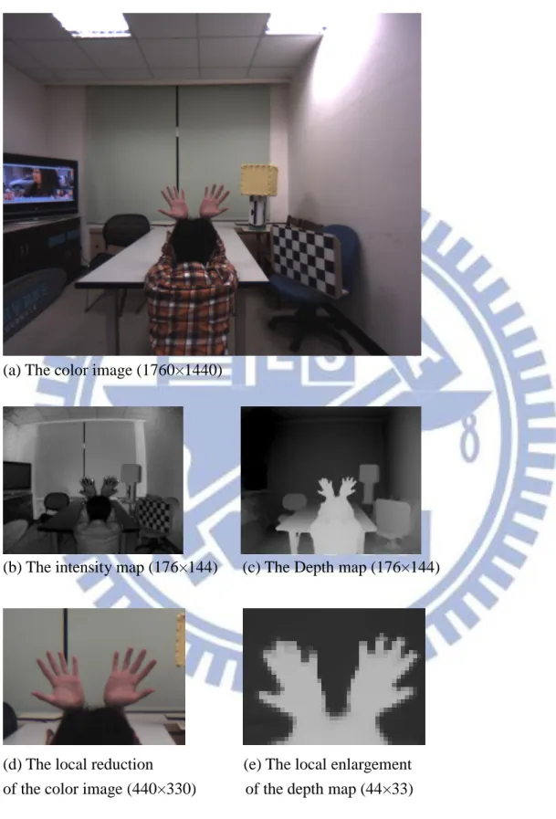
The depth map format of SR4000 is QCIF (Quarter Common Intermediate Format) with resolution 176×144 [14]. The resolution of the depth map is too low to use in practical applications. Such a low resolution depth map cannot provide correct depth information for fine objects. In Figure 16, we take human palms as an example. Obviously, compared with the color image in Figure 16(d), the depth map in Figure 16(e) is too blurred to show fingers

19

clearly.

(a) The color image (1760×1440)

(b) The intensity map (176×144) (c) The Depth map (176×144)

(d) The local reduction (e) The local enlargement of the color image (440×330) of the depth map (44×33)

Figure 16. Images captured by the color and depth camera. Comments in parentheses are the image resolution.

20

3.1.2 The Color Camera

The color image sensor we use is Flea3 USB 3.0, which is show in Figure 17. Flea3 is a color camera produced by Point Grey Company in 2012. Flea3 can capture very high

resolution sequences, and the maximum resolution it supports is 4096 × 2160 [15]. We propose a method to take the advantage of the high resolution color image in Figure 16(a) to compensate for the drawback of the low resolution depth map in Figure 16(c).

The lens mounted on Flea3 color camera is MY110M Ultra Wide Lens which is produced by Theia Technologies Company. The lens uses the Theia's patented Linear Optical Technology® , which allows an ultra-wide field of view without barrel distortion. The

ultra-wide lens makes the field of view of color images to be comparable with the depth map. The Linear Optical Technology® reduces the barrel distortion, so we do not need to do camera distortion calibration on its color images in section 3.2.1.

Figure 17. Point Grey Flea3 USB 3.0 - Color Camera [15]

Figure 18. Theia Technologies MY110M - Ultra Wide Lens [16]

21

3.1.3 Experiment Setup

The experiment setup is shown in Figure 19 (a). We use a tripod head to hold the depth and color cameras. Then, we put both of them in parallel to simplify the problem of alignment between two images taken from different viewpoints. Also, we set the depth and color

cameras as close as possible for two reasons. First, the number of depth pixels is much fewer than the number of color pixels. Therefore, compared with the color pixels, the depth pixels are rare and precious. We put the depth and color cameras close to each other so that the view of the color camera can include the view of the depth camera. After increasing the resolution of the depth map, we would crop the area of the color image to match with the depth map, and thus, every depth pixel is in use. Second, to preserve the quality of the depth map after

alignment, we like to reduce the occlusion regions as much as possible. Reducing the distance between the depth and color camera can reduce the occlusion regions.

We also place two levels perpendicular to each other as shown in Figure 19 (b) to ensure the tripod head is parallel to the ground. This experiment setup can reduce most of the manual errors.

(a) The experiment devices (b) Left is the color camera. Right is the depth camera.

22

3.2 Depth and Color Images Calibration

3.2.1 Camera Distortion Calibration

Most of the lens have non-linear image distortion. The two main lens distortions are the radial distortion and the tangent distortion. The radial distortion is caused by the shape of lens. If the light goes through the lens far from the lens center, it will suffer radial distortion

severely. The tangent distortion is caused by the improper fabrication of the camera.

Figure 20 (a) and (c) are the raw depth and intensity maps captured by the depth camera SR4000 without the camera distortion calibration. Obviously, the ceiling of the intensity map appears to be bended, and so the wall and the desk. Every object far from the lens center suffers from severe radial distortion. Moreover, these distortions in the intensity map also appear in the depth map. This would cause lots of depth value errors in the later process.

Therefore, we use the Camera Calibration Toolbox for Matlab® [17] to do the camera distortion calibration. To detect the lens distortion, the Camera Calibration Toolbox needs various checkerboard images with the checkerboard in different positions. These images are listed in Figure 21. The images in Figure 21 are the intensity maps captured by the depth camera SR4000. As we mentioned in section 3.1.1, because the intensity map is at the same viewpoint of the depth map, we can use the calibration parameters computed for the intensity map to calibrate the camera distortion of the depth map.

Figure 20 (b) and (d) show the results of the camera distortion calibration. We can see that the ceiling, the wall and other objects have been adjusted to align with the objects in the color images. As said in section 3.1.2, the color camera equipped with the MY110M Ultra Wide Lens has no visible barrel distortion. Thus, we do not need to do the camera distortion calibration on the color images.

23

(a) The depth map before calibration (b) The depth map after calibration

(c) The intensity map before calibration (d) The intensity map after calibration

(e) The color image on the scene

24

25

3.2.2 Alignment of Depth and Color Images

Even though we put the depth and color cameras next to each other, the depth map and the color image are still captured at the slightly different viewpoints. In Figure 22, we use alpha blending to show the alignment result of the depth and color images. As shown in Figure 22(a), the foreground and background objects in the depth and the color images do not match at the same position. Because the depth and the color images have different size, the depth map needs to be enlarged about 7.4 times to fit the color image. However, in the depth map refinement algorithm we proposed, the size of the depth map can only be enlarged with the multiple of integer. Therefore, we enlarge 7 times the depth map by nearest-neighbor interpolation and shrink 0.95 times the color image by bilinear interpolation to reach the same goal, enlarging 7.4 times the depth map to fit the color image. After shrinking, the resolution of the color image decreases from 1760×1440 to 1672×1368.

To align the depth and the color images, we need to transform the viewpoint of the depth map to the viewpoint of the color image. The transformation formula is

Pixel Shifted ∝ _Distance1 ∝ Depth Value, (1)

where the pixel shifted is the number of pixels needs to be moved in the horizontal direction, the distance is the distance from the depth camera to the object, and the depth value between 0 to 255 is the intensity value of a depth pixel.

26

(a) The depth map before alignment

(b) The depth map after alignment

27

From eq. (1), the number of pixels shifted equals to zero only if the distance is infinite. However, the distance the depth camera can detect is limited. For our depth camera SR4000, the calibrated range is 0.8 to 8.0 meters, it is impossible to detect objects at infinity. So we have to revise eq.(1) slightly. From eq. (1), because the pixel shifted is proportional to the depth value, we can plot a straight line crossing the origin, if we put the pixel shifted in y-axle and put the depth value in x-axle, as shown in Figure 23(a). Considering the limit of the depth camera, we set the average of background depth values as the intercept in x-axle. Figure 23(b) illustrates the revised transformation formula. Based on the fixed background object, we can shift the depth pixel of foreground objects correctly. The alpha blending of alignment result is shown in Figure 22(b).

(a) The transformation formula of eq. (1) (b) The revised transformation formula

Figure 23. Alignment Algorithm

P ix el Sh if te d Slope = m

Intercept = Background Depth Value Depth Value P ix el Sh if te d Slope = m Depth Value

28

During the process of alignment, how to fill up the occlusion region is a critical problem. General speaking, the occlusion region is parts of the background occluded by the foreground. Hence, it is reasonable to fill in the occlusion region with the depth value of the background in its neighborhood. In our experiment setup, the color camera is on the right side of the depth camera. When we transform the viewpoint from the left to the right, we need to use the depth pixels on the right side of the occlusion region to fill the hole. Nevertheless, for the occlusion region on the external border of the depth map, there is no depth pixel on the right side to fill the hole, as shown in Figure 24(b). In this case, we cannot but extend the depth value of the foreground to fill the hole, as shown in Figure 24(c).

(a) Before alignment (b) After alignment (c) Fill the hole on the border

29

Chapter 4. Depth Map Refinement Algorithm

4.1 Overview of the Proposed Method

We propose a depth map refinement algorithm to increase the resolution of the depth map. The flow diagram is shown in Figure 25. First of all, we slip the color image and its associated depth map into several patches. Then, we use the k-means clustering algorithm to do a simple classification on these image patches. After color image clustering, the depth map classification follows the classification result of the color image. We classify depth map pixels into different classes and correct the wrong depth values. Afterwards, we interpolate the depth pixels of each class to increase the depth map resolution. The depth map refinement algorithm repeats above four steps for all patches of the color image and the corresponding ones on the depth map. Finally, we combine all the processed patches of the depth map into a complete image, and this is the final high resolution depth map.

Figure 25. The flow diagram of the depth refinement algorithm

Patches

Color Images

Clustering

Depth Maps

Clustering

Depth Pixels

Interpolation

High Resolution

Depth Map

30

4.2 Patches

How to determine the size and the position of each patch plays an important role in the proposed depth map refinement algorithm. For a better experimental result, the user needs to decide the patch size manually. We also provide a simpler method to determine the patches automatically. The user can set the patch number of the width and the height, and our program would divide the image evenly as shown in Figure 26.

31

4.3 Color Images Clustering

In color images clustering, we use the k-means clustering algorithm to classify the color image patches. Basically, the objects with the same color would be classified to the same class. However, the noise of the color image would change the color of the object slightly. A tiny difference of the color affects the result of k-means clustering. Therefore, before k-means clustering, we use the median filter to smooth the color image and reduce the difference of similar colors.

Also, because of the light source directions in the environment, the objects with the same color may have different luminance. The difference in luminance may have significant influence on the k-means clustering results. An object of one color may be classified into several fragments. This would cause severe errors in the result of the depth map refinement algorithm. To prevent the effect of illumination, we transform the color image space from RGB to L*a*b* color space. In the L*a*b* color space, the luminance component is isolated in L* space, so we can control the effect of luminance by adjusting the weight of L* space.

32

4.3.1 Median Filter

The median filter is a non-linear filter. The advantage of non-linear filters is that compared with linear filters, they would not distort the edge in an image too much. This is helpful to preserve the image from blurring. Most applications of the median filter are dealing with the salt and pepper noise. Because of the large intensity of the salt and pepper noise, they are dropped in the selecting median value process.

For k-means clustering, we can treat the tiny color differences of identical color in the image as the salt and pepper noise. To produce a better smoothing result, we apply a 7×7 mask median filter to the R, G, and B color components separately. The result of the median filter is shown in Figure 27(b). After the median filter, the object texture is blurred. It seems that the image losses some details, but this would benefit the k-means clustering result shown in Figure 36.

(a) Before the median filter (b) After the median filter

33

4.3.2 L*a*b* Color Space

Luminance has a lot of influences on the display of color. We take Figure 28 as an example. Figure 28(a) is a set of colored paint samples with different luminance [18]. The upper part is in the shadow, and the lower part is in the sunshine. Figure 28(b) is patches extracted from Figure 28(a). Figure 28(c) is the patches of the second column in Figure 28(b). Now, we want to identify the object edges. When we look at the whole color paint samples in Figure 28(a), there are four colors. However, if we look at Figure 28(b), there seem to be eight colors. It is the illumination that changes the perceived colors. Thus, the illumination can also confuse the k-means clustering. So, we transform the color space from RGB to the L*a*b* color space to reduce this effect.

(a) A set of colored paint samples

(b) Patches cropped from (a) (c) Patches cropped from (b)

34

In Figure 29, we compare three common color spaces RGB, HSV and CIE Lab and use the receiver operating characteristic (ROC) curves to demonstrate that the CIE Lab color space is the most suitable color space for edge classification.

A ROC curve shows the accuracy of the binary classifier. The true positive fraction is the number of correctly classified reflectance edges against the total number of reflectance edges. The true positive and false positive fractions are chosen to plot ROC curves. The area under the ROC curve (AUC) describes the discrimination ability of a binary classifier. If the AUC is close to 1, it means that the classification result is more accurate. However, if the AUC is close to 0.5, it shows that the behavior of classifier is similar to the random guess.

As Figure 29(b) and (c) shows, the value (V) component of HSV and the luminance (L) component of CIE Lab are not good for edge classification. The result is reasonable. Because the value component of HSV and luminance component of CIE Lab represent the brightness of the object, which is a combination of environment and object reflectance. They contribute less to the color classification. However, in Figure 29(a), the RGB color space has no single significant channel corresponding to the brightness, so three ROC curves get close. In TABLE 1, the AUC of HSV-V and CIE Lab-L are close to 0.5, and the other channels are near 1. The AUC of RGB does not have such a characteristic. This is the reason that we convert the color space from RGB to L*a*b*.

(a) RGB (b) HSV (c) CIE Lab

35

The display of sRGB in the L*a*b* color space is shown in Figure 30(a). Dimension L* means luminance or brightness and its ranges from 0 to 100 displays the black color and L*=100 represents the white color. Dimensions a* and b* stand for the color-opponents and range from -127 to 128. The asterisk (*) indicates that the L*a*b* color space is the

non-linear coordinate axis. Figure 30(b), (c) and (d) show the slices of sRGB in the L*a*b* TABLE 1. Channels and their AUCs for outdoor and indoor scenes [18]

36

color space with different L*. Obviously, with a larger L* value, the color would become brighter.

(a) sRGB in L*a*b* color space (b) sRGB (L*=1)

(c) sRGB (L*=50) (d) sRGB (L*=99)

37

To reduce the influence of illumination, the most intuitional method is to remove the L* axis as shown in Figure 31. However, luminance is not only on behalf of brightness of color, but stand for black and white. As mentioned earlier, L*=0 is the black color and L*=100 is the white color. If we remove the L* axis entirely, the k-means clustering cannot differentiate black and white anymore.

To differentiate black and white and reduce the luminance of colors simultaneously, we revise the idea of Figure 31 and show it in Figure 32. We set 20% of max L* as the upper bound of black and set 80% of max L* as the lower bound of white. The L* axis is separated into three parts, which are white, color and black. Then, we unify the intensity value of L* to the mean value in each class. The revised distribution shown in Figure 32(b) is better for k-means clustering purpose.

(a) Before removing L* (b) After removing L*

Figure 31. Remove the L* axis from the L*a*b* color space

a*

L*

b*

a*

38

(a) Before unifying L* (b) After unifying L*

Figure 32. Unify the intensity of L*

a*,b*

L*

a*,b*

L*

39

4.3.3 Segmentation and K-means Clustering

For the proposed depth map refinement algorithm, the color image segmentation result is critical. We first try a popular image matting method “Learning Based Digital Matting” [20] to separate the foreground from the background. The image matting result is shown in Figure 33. The user needs to plot a trimap manually as shown in Figure 33(b) to roughly indicate the boundary between the foreground and the background. Then, the Learning Based Digital Matting method uses the trimap to produce a matting result as shown in Figure 33(c). Another image matting result with different dataset is shown in Figure 34

(a) The color image (b) The trimap

(c) The matting result (d) The enlargement of (a) and (c)

40

As Figure 33(d) and Figure 34(d) show, the finger part extraction has noticeable distortion. For a better matting result, the user needs to plot the trimap with care. The process of plotting an explicit trimap is time-consuming and inefficient, and the results are not up to our expectation. Hence, we adopt a simpler algorithm “k-means clustering” to do color image clustering.

The k-means clustering algorithm is a critical step in color image classification. The purpose of color image classification is for later region alignment and interpolation. However, a sophisticated image segmentation algorithm costs a lot of computation time and does not

(a) The color image (b) The trimap

(c) The matting result (d) The enlargement of (a) and (c)

41

serve for our purpose. So, we choose a simple clustering method, k-means clustering, to do image segmentation. The dataset for k-means clustering is pixels of the color image with three dimensions, L*, a* and b* color components. The process of k-means clustering is as follows. Step1. Decide the number of clusters and the locations of initial means.

Step2. Compute the distance from every piece of data to the mean. Step3. Classify the data to the cluster with shortest distance. Step4. Compute the new mean of each cluster, and go to Step2.

The k-mean clustering algorithm iterates these steps several times, and the user can decide the number of iteration. If the number of iteration is set too few, the k-means algorithm does not have significant time to converge to the steady state. On the other hand, if the

number of iteration is set too high, the k-means clustering may go to over-fit.

Although k-means clustering is very simple, there are two key factors that dominate the performance. One is the number of the clusters and the other is the locations of initial centers. A reasonable number of the cluster should be decided individually for every single patch. To simplify the process, we set the number of the cluster to four. The initial centers (mean locations) play an important role in the result of k-means clustering. The suitable locations of initial means can increase the accuracy of k-means clustering. In our program, with no prior information, the initial means are uniformly selected.

In Figure 35, different color makes the region (cluster) produced by the k-means clustering. For pixels classified into the same cluster, they are pained by the same color. An example of the classification result is shown in Figure 35.

42

(a) The patch of the color image (b) The k-means clustering result

Figure 35. The k-means clustering result

(a) Without the median filter (b) With the median filter

43

4.4 Depth Map Clustering

The median priced depth cameras nowadays still cannot produce high resolution depth maps. The raw depth maps often contain noise and are blurred. Enlarging the raw depth maps directly is unable to create sharp and correct object boundaries compatible with those of color images. Therefore, we do depth maps clustering before depth pixels interpolation to increase the correspondence of object boundaries. Because the depth maps have no texture information of objects and suffer from low resolution, the depth maps segmentation uses the color image clustering results to classify depth pixels.

In our experiments, the depth map needs to be enlarged 7 times to match the size of the color images. Instead of using the conventional interpolation method, we place the original depth pixels on the pixel grid of the color image, and thus the depth map becomes sparse. The sparse depth map is shown in Figure 37(b). Referring to the result of k-means clustering, the sparse depth pixels are classified into different clusters. There are some depth pixels with unreasonable depth value in a cluster. Hence, we collect the depth pixel statistics to find the dominant and the rare depth value in a cluster. In general, the rare depth value in a cluster is very different from the dominant value, and possible to be noise of the depth map. To correct them, we replace the rare depth values with the dominant depth value. Then, we obtain a corrected spare depth map. We will elaborate this procedure step by step in the following sub-sections.

4.4.1 Spreading

The raw depth map needs to be enlarged 7 times to match the color image size. The conventional interpolation method cannot correct the depth map boundary errors and would create a blurred image. To solve these problems, we spread the original depth pixels on the color image pixel grid instead of interpolation. The sparse depth map is shown in Figure 37(b), and the corresponding color image is shown in Figure 37(a). There are 6 blank pixels between

44

two spread depth pixels in horizontal and vertical directions. These blank pixels will be filled up appropriately in section 4.5 Depth Pixels Interpolation.

(a) The color image with sparse depth pixels

(b) The sparse depth map

45

4.4.2 Classification

Because of its low resolution, the original depth map is sparse on the high resolution grid as discussed earlier. An example is shown in Figure 38(c). We would like to refer to the edge of the color image to revise the edge of the depth map. Thus, the depth maps clusters come from the color images clusters. Figure 38(a) illustrates the sparse depth pixels and the corresponding color image. The blue dots are the foreground pixels of the depth map in Figure 38(c). The yellow dots represent the background pixels. Clearly, some of the blue dots do not match the shape of the object in the color image. The red dots in Figure 38(b) are the depth pixels that need to be modified.

The sizes of the depth map and the color image are different. To construct the correct object edges on the depth map, we extract the pixels from the color images clusters based on the locations of the sparse depth pixels. This process can be regarded as a down sampling procedure which reduces Figure 35(b) to Figure 39(a). Compared with Figure 39(b), the raw depth map, Figure 39(a) shows sharp object edges. We thus take Figure 39(a) as the reference to classify the depth pixels in Figure 39(b) into clusters and thus correct the blurred object edges.

(a) The original depth pixels (b) The correct depth pixels (c) The depth map

46

4.4.3 Statistics

After knowing the correct object edges on the depth map, we need to modify the incorrect depth pixels. To correct these depth pixels, there are two problems we have to deal with. One is how to identify the depth pixel to be modified, and the other is the “correct” depth value which is used to replace the wrong depth pixel. In our algorithm, we use a statistical method to solve these two problems at the same time.

Referring to the down-sampling clusters of the color image, we classify the depth pixels into appropriate clusters. The procedure was described in the previous sub-section. For each class, we collect the distribution of depth values, that is, histogram in Figure 40(c). Generally, there is only one object in one class, so the depth values in each class should be close to each other. In Figure 40(c), we can see that there is a dominant depth value and some noise-like depth values. The depth pixels with these rare depth values are judged incorrect. They may be due to the noise in the depth map or the blurred edges. Then, the dominant depth value is the depth value used to modify the wrong depth pixels.

(a) The classification result (b) The depth map

47

(a) The classification result (b) The depth map

(c) The histogram of depth pixels

Figure 40. The histogram of depth pixels

48

4.4.4 Correction

As described in the previous sub-section, we modify the incorrect depth values by the dominant depth value. However, the classification result of color images is not all perfect. Occasionally, there are two or more objects classified to the same cluster. In this case, the dominant depth value is not unique anymore. Also, if the depth camera captures an image of gradual depth variation, such as the side of a wall, then the depth map of the wall contains many depth values. This is a special case we need to discuss.

To solve these two cases simultaneously, we extend the definition of the dominant depth value. Previously, we choose the depth value with the maximum number of pixels as the dominant depth value. Now, we extend the definition. If the depth values with the number of pixels more than the half of the maximum number of pixels, they become the second

dominant depth value. In this new definition, there may be several dominant depth values in one class. Every dominant value is a candidate to replace the wrong depth value. Moreover, the depth values greater than or within 5 intensity levels of the dominant depth value are preserved. This would keep the slight different depth values and make the depth map look more natural. The corrected result is shown in Figure 41 and Figure 42.

49

(a) The depth map (b) The histogram of depth pixels

(c) The depth map (d) The histogram of depth pixels

50

(a) Before correcting

(b) After correcting

51

4.5 Depth Pixels Interpolation

As mentioned in section 4.4.1, there are 6 blank pixels between two spread depth pixels in the horizontal and vertical directions. After getting the corrected depth map, we begin to fill up these blank pixels. Even though we have the corrected depth map, there are a large

difference between the resolutions of the depth map and the color image. If we interpolate the depth map directly, we would get an enlarged blurred map. Therefore, we need to fill up the blank pixels class by class.

According to color image clustering, we split the corrected depth map into several classes. For each class, we fill up the blank pixels individually. Before interpolation, we dilate the depth map to make sure the quality of interpolation. Then, after interpolation, we filter out the blurred edge and combine all results of classes. The high resolution depth map is

52

4.5.1 Separation

We want to fill up the blank pixels class by class, so we need to separate the depth map into several parts according to color image clusters. If the depth pixels correspond to the same cluster, they are marked as the identical part. The separation result is shown in Figure 43. The corrected depth map in Figure 43(b) is separated into three different parts as shown in Figure 43(c), (d) and (e).

(a) The classification result (b) The corrected depth map

(c) The palm (d) The background (e) The head

53

4.5.2 Expansion

Before interpolation, we expand the depth pixels of each class. The purpose is to fill up all possible foreground pixels. If we perform the ordinary interpolation, the object edges are often blurred. This is because the depth value changes along the edge are sharp. The typical bi-linear interpolation for example cannot produce such a sharp edge. In this ordinary interpolation process, the depth pixels along edges are computed from the average of the background and the foreground depth values. Expansion of the foreground depth pixels extends the dominant depth value to the outer region. Then, we have to remove the background part, and then the sharp edge is preserved. The expansion result is shown in Figure 44.

54

4.5.3 Interpolation and Reshaping

To keep gradual variation in a depth map, we use linear interpolation to fill up blank pixels of every class. The depth value of nearby pixels can thus change gradually except on the edges. So, linear interpolation is suitable to compute the depth value changing gradually. As for the edges, we remove the unused part to preserve the sharp edges. The k-means clustering result of the color image can provide clear shapes of objects. Referring to the k-means clustering result, we can prune the expanded and interpolated depth map precisely. The reshaping result is shown in Figure 45.

Figure 45. Reshape the blurred edge

55

4.5.4 Combination

Finally, we combine the results of all classes (clusters) to complete one patch of the high resolution depth map. The result is shown in Figure 46.

(a) The color image (b) The result of one patch

56

4.6 Experimental Results

The experiment result with different dataset is shown in Figure 47, Figure 48, and Figure 49. We provide two experimental results for each dataset. They are processed with automatic and manual patch decision respectively. Compared with Figure 47(b), Figure 47(d) has less broken holes on the boundary of patches. Figure 47(d) has better depth map quality than conventional nearest interpolation method shown in Figure 47(c). The enlargement of detail in Figure 47(c) and (d) is shown in Figure 47(e) and Figure 47(f). Obviously, in Figure 47(f), the depth map of the yellow cube looks more like the shape of it in the color image. The palm in Figure 48(f) and the chair in Figure 49(f) also have better depth map quality than the nearest interpolation method.

57

(a) The color image (b) The automatic result

(c) The nearest interpolation result (d) The manual result

(e) The enlargement of nearest interpolation (f) The enlargement of manual result result

58

(a) The color image (b) The automatic result

(c) The nearest interpolation result (d) The manual result

(e) The enlargement of nearest interpolation (f) The enlargement of manual result result

59

(a) The color image (b) The automatic result

(c) The nearest interpolation result (d) The manual result

(e) The enlargement of nearest interpolation (f) The enlargement of manual result result

60

Chapter 5. Conclusions and Future Work

5.1 Conclusions

The drawback of depth-sensor depth maps is its low resolution. We propose a depth map refinement algorithm that uses high resolution color images to increase the resolution of depth maps. The k-means clustering results of color images is very important to identify the edges of objects. Proper selected edges on color images can sharpen the edges on depth maps and prove the depth maps quality. The k-means clustering algorithm has better clustering results in a smaller, local region, so we split the whole image into a number of patches. The position and size of patches are critical for producing good results in k-means clustering. Hence, the layout of patches is a significant step in depth map refinement algorithm. For better results, we need to decide the position of patches for individual picture. At the end, we demonstrate a high resolution good quality depth map based on the combination of all processed patches.

5.2 Future Work

As mentioned earlier, the position and size of patches have great influences on the result of depth refinement algorithm. In this thesis, to generate a good quality depth map, we need to tune the patches for each image. Such a manual process work is not efficient to handle video sequences. Thus, a method to decide the layout of patches automatically is essential in the future. Or, we need a better and automatic segmentation algorithm for classification purpose.

61

Bibliography

[1] J. H. Cho, K. H. Lee, and K. Aizawa, "Enhancement of Depth Maps With Alpha Channel Estimation for 3-D Video," Ieee Journal of Selected Topics in Signal Processing, vol. 6, pp. 483-494, Sept 2012. [2] "3DV data: Newspaper," Gwangju Institute of Science and Technology (GIST), Republic of Korea. [3] Kinect, http://en.wikipedia.org/wiki/Kinect

[4] K. Xu, J. Zhou, and Z. Wang, "A Method of Hole-filling for the Depth Map Generated by Kinect with Moving Objects Detection," presented at the 2012 Ieee International Symposium on Broadband

Multimedia Systems and Broadcasting (Bmsb), June 2012.

[5] S. Matyunin, D. Vatolin, Y. Berdnikov, and M. Smirnov, "Temporal Filtering for Depth Maps Generated by Kinect Depth Camera," presented at the 2011 3dtv Conference: The True Vision - Capture, Transmission

and Display of 3d Video (3dtv-Con), May 2011.

[6] Time-of-flight camera, http://en.wikipedia.org/wiki/Time-of-flight_camera

[7] PMD-Sensor, http://de.wikipedia.org/wiki/PMD-Sensor

[8] H. Schafer, F. Lenzen, and C. S. Garbe, "Depth and Intensity Based Edge Detection in Time-of-Flight Images," presented at the 2013 International Conference on 3D Vision - 3DV 2013, Seattle, WA, USA, June 2013.

[9] D. Ferstl, R. Ranftl, M. Ruther, and H. Bischof, "Multi-modality depth map fusion using primal-dual optimization," presented at the 2013 IEEE International Conference on Computational Photography (ICCP), Cambridge, MA, April 2013.

[10] Multi-Modality Depth Map Fusion,

http://rvlab.icg.tugraz.at/project_page/project_tofusion/project_multi_modality_fusion.html

[11] J. Park, H. Kim, Y.-W. Tai, M. S. Brown, and I. Kweon, "High Quality DepthMap Upsampling for 3D-TOF Cameras," presented at the 2011 IEEE International Conference on Computer Vision (ICCV), Barcelona, Nov 2011.

62

presented at the 2012 IEEE International Conference on Robotics and Automation (ICRA), Saint Paul, MN, May 2012.

[13] MESA Imaging - SR4000/SR4500 User Manual [14] MESA Imaging - SR4000 Data Sheet

[15] Point Grey - Flea3 USB 3.0 Product Datasheet

[16] Theia Technologies - MY110M http://www.theiatech.com/products.php?lens=MY110

[17] J.-Y. Bouguet, "Camera Calibration Toolbox for Matlab® ," Computer Vision Research Group Dept. of Electrical Engineering California Institute of Technology, 2013.

http://www.vision.caltech.edu/bouguetj/calib_doc/

[18] E. Reinhard, E. A. Khan, A. O. Akyüz, and G. M. Johnson, Color Imaging Fundamentals and Applications. A K Peters/CRC Press, 2008.

[19] G. Hoffmann, "CIELab Color Space," 2003. http://docs-hoffmann.de/

[20] Y. Zheng and C. Kambhamettu, "Learning Based Digital Matting," presented at the 2009 IEEE 12th

International Conference on Computer Vision (ICCV), Kyoto, Sept 2009.

http://www.mathworks.com/matlabcentral/fileexchange/31412-learning-based-digital-matting/content/lear ningBasedMatting.zip