韋柏分配下規格下限與X-bar 管制圖之經濟設計 - 政大學術集成

全文

(1)國立政治大學統計學系碩士學位論文. 指導教授：. 楊素芬博士. 韋柏分配下規格下限與治管制圖之經濟設計政 X-bar. 大. 立 of specification limit and X-bar Economic design. ‧ 國. 學. control chart under Weibull distribution. ‧. n. er. io. sit. y. Nat. al. Ch. engchi. i n U. v. 研究生：蔡瑋倫撰中華民國一百零二年六月.

(2) 謝辭研究生活即將到了尾聲，這段日子我過得很充實，除了學到了許多統計品管的知識，也學到了待人處事以及作研究的態度與方法。首先要感謝我的指導教授. 楊素芬教授，感謝老師這些日子的用心指導與鼓勵，. 讓我能全力面對挑戰。老師的認真教學以及專注研究的態度亦讓我獲益良多。感謝我的口試委員曾勝滄教授以及唐正教授，謝謝兩位老師在百忙之中仍抽空閱讀本論文並給予許多珍貴的建議與想法，讓本論文能更趨完善。感謝教了我許多統計研究方法、閱讀論文訣竅以及寫報告技巧的學長姊：伊萱、鈞遠、雨築、家玲以及至芬。感謝一路陪伴我的同學，特別是佳宏與依潔，有你們兩. 政治大. 位的鼓勵與扶持，幫助我克服許多困難以及難題。. 立. 最後要謝謝我的家人，有你們的鼓勵與支持，全心全意的當我的後盾，我才能有. ‧ 國. 學. 幸完成碩士班的學業以及本論文。未來的日子我會更加努力，期許自己能讓你們過更. ‧. 舒適的日子。. 本研究承蒙行政院國家科學委員會補助，計畫編號 NSC100-2118-M-004-003-MY2，. n. al. er. io. sit. y. Nat. 謹此致謝。. Ch. engchi. i n U. v. 蔡瑋倫謹致中華民國一百零二年六月 I.

(3) Abstract To determine the economic design of control charts and the specification limits with minimum cost are two separate issues in previous research areas. In this study, we proposed a method to determine the optimal design parameters of X control charts and the specification limits simultaneously from an economic viewpoint. We also consider two types of X control charts: one is the economic X control chart and the other is the economic statistical X control chart. We obtain the optimal results by minimizing the expected cost per unit time for the-larger-the-better quality characteristic with a Weibull distribution. We consider the asymmetric control limits because of the asymmetric feature of the Weibull. 政治大. distribution. Also, we are considering the difference between monitoring the process by. 立. using an economic statistical X control chart and conducting a complete inspection plan.. ‧ 國. 學. Which way is better, process control or inspection plan?. ‧. In our data analysis of the two types of X control chart, we find that the optimal expected cost per unit time with complete inspection is lower than without complete. y. Nat. io. sit. inspection. This is because the coefficient of Taguchi’s quadratic loss function we set is too. n. al. er. small. And the analysis shows us the significant parameters for the optimal expected cost per unit time and design parameters.. Ch. engchi. i n U. v. At last, in our numerical examples for two different types of X control chart, we find that the performance of the economic X control chart is as good as the economic statistical one. However, we suggest the producer use the economic statistical X control chart with a complete inspection plan to obtain a lower expected cost per unit time and larger power of the control chart.. Keywords: Economic design; X control chart; Specification limit; Weibull distribution. II.

(4) CONTENT CHAPTER 1. INTRODUCTION .......................................................................................... 1 1.1 Research Motivation ....................................................................................................... 1 1.2 Literature Review ........................................................................................................... 2 1.3 Research Method ............................................................................................................ 4 CHAPTER 2. ECONOMIC DESIGN OF A X CONTROL CHART FOR A PROCESS WITH WEIBULL DATA............................................................ 6 2.1 Approximated In-Control Sampling Distribution of the X under Weibull Distribution6 2.2 Approximated Out-of-Control Sampling Distribution of X under Weibull. 政治大. Distribution ..................................................................................................................... 9. 立. 2.3 Construction of Economic X Probability Chart Based on X Sampling Distribution9. ‧ 國. 學. 2.4 The Calculation of  and  ...................................................................................... 10. ‧. 2.5 Derivation of Expected Cycle Time .............................................................................. 10 2.6 Derivation of the Expected Cycle Cost ......................................................................... 12. y. Nat. io. sit. 2.7 Determination of the Optimum Sampling Interval of the Economic X Control Chart14. n. al. er. 2.8 Data Analysis and Resulting Comparison to Different Out-of-Control Distributions .. 15. i n U. v. CHAPTER 3. DESIGN OF ECONOMIC X CHART AND INSPECTION SPECIFICATION LIMIT FOR A PROCESS WITH WEIBULL DATA 20. Ch. engchi. 3.1 Derivation of the Expected Cycle Cost ......................................................................... 20 3.2 Determination of the Optimum Specification Limit and Design Parameters of the Economic X Control Chart ....................................................................................... 22 3.3 Data Analysis and the Result Comparisons with and without the Inspection Plan ....... 22 3.4 An Example ................................................................................................................... 28 3.4.1 Data ..................................................................................................................... 28 3.4.2 Estimating the in-control parameters of the Weibull distribution ....................... 29 3.4.3 Simulation Data for Out-of-control Distribution ................................................ 30 3.4.4 Constructing the economic X control chart and inspection plan .................... 31 III.

(5) CHAPTER 4. ECONOMIC STATISTICAL DESIGN OF THE X CHART FOR THE PROCESS USING WEIBULL DATA ............................................... 33 4.1 Construction of the Economic Statistical X Chart Based on the X Sampling Distribution and Determination of the Optimum Design Parameters of the Economic Statistical X Control Chart ........................................................................................ 33 4.2 Data Analysis and Result Comparisons for the Different Out-of-control Distributions 34 CHAPTER 5. DETERMINATION OF THE INSPECTION SPECIFICATION AND ECONOMIC STATISTICAL X CHART FOR A PROCESS WITH WEIBULL DATA ......................................................................................... 40 5.1 Determination of the Optimum Specification Limit and Design Parameters of the Economic Statistical X Control Chart ...................................................................... 40. 政治大. 5.2 Data Analysis and Result Comparisons with and without the Inspection Plan ............. 40. 立. 5.3 An Example ................................................................................................................... 47. ‧ 國. 學. 5.3.1 Obtaining the range of the UCL and LCL ........................................................... 47. ‧. 5.3.2 Constructing the economic statistical X control chart and inspection plan ... 47 5.3.3 Comparison of the economic X control chart with inspection plan and the. y. Nat. sit. economic statistical X control chart with inspection plan ............................... 49. er. io. CHAPTER 6. COSTS COMPARISON OF THE PROCESS QUALITY CONTROL AND PRODUCT INSPECTION ................................................................. 51. al. n. v i n 6.1 Derivation of The Expected C Cycle ........................................................................ 51 h eCost ngchi U 6.1.1 The cost for process control in the observing time OT ........................................ 51 6.1.2 The total cost for product inspection in observing time OT ................................ 52 6.2 Data Analysis and Comparing the Results with Different In-control Weibull Distributions ................................................................................................................. 53 6.2.1 Cost for process control ....................................................................................... 53 6.2.2 Cost for production inspection ............................................................................ 59 6.3 Analysis for the Cost Difference.................................................................................... 64. CHAPTER 7. CONCLUSION AND RECOMMENDATIONS FOR FUTURE STUDY76 REFERENCES ....................................................................................................................... 78 IV.

(6) LIST OF TABLES Table 2- 1. The Simulated Data for Weibul(2, 2) ...................................................................... 8 Table 2- 2. The Summary Table for Goodness of Fit ................................................................ 9 Table 2- 3. The Level of Each Parameter ................................................................................ 15 Table 2- 4. Parameters for Each Level Combination .............................................................. 16 Table 2- 5. Optimal Solutions for Each Level Combination ................................................... 17 Table 2- 6. The Values of EA* for Each Parameter. .............................................................. 19 Table 2- 7. The Significant Parameters and Their Relationship of Each Design Parameter and EA..................................................................................................................................... 19. 政治大. Table 3- 1. The Level of Each Parameter ................................................................................ 22. 立. Table 3- 2. Parameters for Each Level Combination .............................................................. 23. ‧ 國. 學. Table 3- 3. Optimal Solutions for Each Level Combination ................................................... 25. ‧. Table 3- 4. The Values of h * for Each Parameter. ............................................................... 26. sit. y. Nat. Table 3- 5. The Values of EA L * for Each Parameter ........................................................... 26. n. al. er. io. Table 3- 6. Economic X Chart for Products Without Inspection Plan Compares to. i n U. v. Economic X Chart for Products With Inspection Plan. ................................................ 27. Ch. engchi. Table 3- 7. The Significant Parameters and Their Relationship of Each Design Parameter and EAL ................................................................................................................................... 28 Table 3- 8. Breaking Stress of Carbon Fibres. ........................................................................ 29 Table 3- 9. Simulated Data From Out-of-Control Distribution ............................................... 30 Table 4- 1. Optimal Solutions for Each Level Combination ................................................... 35 Table 4- 2. The Values of LCL * for Each Parameter ........................................................... 36 Table 4- 3. The Values of UCL * for Each Parameter ........................................................... 37 Table 4- 4. The Values of EA * for Each Parameter .............................................................. 37 Table 4- 5. The Values of  * for Each Parameter ............................................................... 38 V.

(7) Table 4- 6. The Significant Parameters and Their Relationship of Each Design Parameter and EA..................................................................................................................................... 38 Table 4- 7. Economic X Chart for Products Without Inspection Plan Compare to Economic Statistical X Chart for Products Without Inspection Plan ............................................ 39 Table 5- 1. Optimal Solutions for Each Level Combination ................................................... 42 Table 5- 2. The Values of h * for Each Parameter ................................................................ 43 Table 5- 3. The Values of EA L * for Each Parameter ........................................................... 43 Table 5- 4. The Values of  * for Each Parameter ............................................................... 44. 政治大. Table 5- 5. The Significant Parameters and Their Relationship of Each Design Parameter and. 立. EAL ................................................................................................................................... 44. ‧ 國. 學. Table 5- 6. Economic Statistical X Control Chart for Products Without Inspection Plan Compare to Economic Statistical X Control Chart for Products With Inspection Plan 45. ‧. Table 5- 7. Economic X Control Chart for Products With Inspection Plan Compare to. Nat. sit. y. Economic Statistical X Control Chart for Products With Inspection Plan ................... 46. n. al. er. io. Table 5- 8. The Significant Parameters of Each Design Parameter and EA (or EAL) for. i n U. v. Different Economic Design of X Control Chart With or Without Inspection Plan ...... 46. Ch. engchi. Table 5- 9. Comparison of Economic X Chart and Economic Statistical X Chart .......... 49 Table 6- 1. The Level of Each Parameter of Process Control ................................................. 53 Table 6- 2. Parameters for Each Level Combination of Process Control................................ 54 Table 6- 3. Optimal Solutions for Each Level Combination of Process Control .................... 56 Table 6- 4. The Values of h * for Each Parameter ................................................................ 57 Table 6- 5. The Values of UCL * for Each Parameter .......................................................... 57 Table 6- 6. The Values of LCL * for Each Parameter .......................................................... 57 Table 6- 7. The Values of EC PC * for Each Parameter ......................................................... 58 VI.

(8) Table 6- 8. The Values of  * for Each Parameter ............................................................... 58 Table 6- 9. The Level of Each Parameter of Product Inspection ............................................. 59 Table 6- 10. Parameters for Each Level Combination of Product Inspection ......................... 60 Table 6- 11. Optimal Solutions for Each Level Combination of Product Inspection .............. 63 Table 6- 12. The Values of LSL * for Each Parameter ......................................................... 64 Table 6- 13. The Values of yield * for Each Parameter ........................................................ 64 Table 6- 14. The Values of EC Ins * for Each Parameter ....................................................... 64 Table 6- 15. The Values of EC Ins *  EC PC * for Each Level Combination with Common. 政治大 Parameters ........................................................................................................................ 65 立. ‧ 國. 學. Table 6- 16. The Values of EC Ins *  EC PC * for Each Common Parameter. ......................... 66 Table 6- 17. The Values of EC Ins *  EC PC * for Each Uncommon Parameter ..................... 68. ‧. sit. y. Nat. Table 6- 18. The Values of EC Ins *  EC PC * for Each Parameter in Process Control. .......... 69. n. al. er. io. Table 6- 19. The Values of EC Ins *  EC PC * for (A, Rn, IC) of Production Inspection. ....... 72. i n U. v. Table 6- 20. The Relationship Between the Significant Parameter and ECPC* ...................... 75. Ch. engchi. Table 6- 21. The Relationship Between the Significant Parameter and ECIns*....................... 75 Table 6- 22. The Relationship Between the Significant Parameter and EC Ins *  EC PC * ..... 75. VII.

(9) LIST OF FIGURES Figure 2- 1.Continuous Process Cycle. ................................................................................... 12 Figure 3- 1. The Weibull Distribution and Taguchi’s Quadratic Loss Function With Inspection Specification Limit ......................................................................................... 20 Figure 3- 2. The Probability Plot for Weibull Distribution ..................................................... 30 Figure 3- 3. Economic X Control Chart (Phase I) ............................................................... 31 Figure 3- 4. Economic X Control Chart (Phase II) .............................................................. 32 Figure 3- 5. The Relationship Between the In-control and Out-of-control Distribution and the Lower Specification Limit ............................................................................................... 32. 政治大. Figure 5- 1. Economic Statistical X Control Chart (Phase I) .............................................. 48. 立. Figure 5- 2. Economic Statistical X Control Chart (Phase II) ............................................. 48. ‧ 國. 學. Figure 6- 1. The Generalized Cycle Time for Process Control ............................................... 52 Figure 6- 2. The Observing Time for Product Inspection ....................................................... 52. ‧. Figure 6- 3. The Response Graph for EC Ins *  EC PC * for Each Common Parameter. ........ 66. y. Nat. io. sit. Figure 6- 4. Graph of ECPC and ECIns in View of  .............................................................. 66. n. al. er. Figure 6- 5. Graph of ECPC and ECIns in View of OT ............................................................. 67. Ch. i n U. v. Figure 6- 6. The Response Graph for EC Ins *  EC PC * for Each Parameters in Process. engchi. Control. ............................................................................................................................. 69 Figure 6- 7. Graph of ECPC and ECIns in View of (C0, C1) ...................................................... 70 Figure 6- 8. Regression Line of ECIns-ECPC and C1-C0 .......................................................... 71 Figure 6- 9. Graph of ECPC and ECIns in View of δ2 ............................................................... 71 Figure 6- 10. The Response Graph of EC Ins *  EC PC * for (A, Rn, IC) of Production Inspection. ........................................................................................................................ 72 Figure 6- 11. Graph of ECPC and ECIns for A .......................................................................... 73 Figure 6- 12. Graph of ECPC and ECIns for Rn......................................................................... 73 Figure 6- 13. Graph of ECPC and ECIns in for IC .................................................................... 74 VIII.

(10) CHAPTER 1. INTRODUCTION 1.1 Research Motivation Control charts and inspections are two common methods used to control process quality. Quality engineers can use statistical process control techniques, such as control charts, to improve quality or to ensure that products meet specifications by conducting inspections. If we wish to use control charts, we must first select the design parameters, such as the sample size, sampling time, and control limits. Economic design is a good approach for assisting in the determination of design parameters from an economic viewpoint. However, we may wish. 政治大 Most articles on the economic design of control charts and determination of product 立. to reduce quality loss resulting from product defects by conducting complete inspections.. ‧ 國. 學. specifications consider quality variables that follow normal distributions. In this article, we apply the Weibull distribution to the “larger-the-better” quality characteristics. Consequently,. ‧. we are only required to locate an optimal lower specification limit of the interested quality. sit. y. Nat. variable. In technology industries, the “larger-the-better” quality characteristics are very. io. er. common, such as a long product life for light emitting diodes (LEDs) is preferable. We can. al. determine optimal specification limit by minimizing the production cost of products.. n. v i n C hlimit and design parameters Determining the product specification of a control chart plays an engchi U important role in quality monitoring and minimal production cost. In this study, we concurrently determine the product specification limit and design parameters of a control chart by minimizing the expected production cost of products per unit time. Because the exact distribution of the sample mean for the Weibull distribution is difficult to derive, we apply a simple technique to approximate its probability density function (pdf) or cumulative distribution function (cdf) of the sample mean. For various shifts of mean and variance and under certain statistical performance target, we design the economic and economic statistical. X control charts. We included the costs of process control and production inspections in the production cost model, and then we minimized the cost model to determine the optimal 1.

(11) design parameters of the X control chart and the lower specification limit for a product with complete inspection plan. 1.2 Literature Review Economic design of control charts is a popular and effective approach for improving outgoing product quality and lowering production costs. Duncan (1956) first proposed the economic design of the X chart with only a single special cause. He designed the X control chart that minimizes all production costs in a production cycle. He considered a continuous process, which means the process continued while engineers searched for an assignable cause. Duncan (1971) generalized his single assignable cause model to design of. 政治大. the X chart with multiple special causes. Montgomery (1980) provided a review and. 立. literature survey for the economic design of control charts. Panagos, Heikes, and. ‧ 國. 學. Montgomery (1985) presented two models considering the continuous and discontinuous manufacturing processes, respectively. Lorenzen and Vance (1986) generalized the Duncan. ‧. (1956) model to include two dummy variables to present whether the process continued or. Nat. sit. y. stopped while the engineer search for an assignable cause and repair the out-of-control. n. al. er. io. process. Elsayed and Chen (1994) developed the first economic design of X chart, based. i n U. v. on the Taguchi quadratic loss function. Yang (1997) presented a joint economic design of X. Ch. engchi. and S charts with two assignable causes using the Taguchi quadratic loss function. Yang (1998) addressed a statistically constrained economic S control chart that including the Taguchi quadratic loss function. Chou et al. (2002) studied an economic statistical design of multivariate control charts using quality loss function for monitoring the process mean vector and covariance matrix simultaneously. Yang and Rahim (2005) presented a cost model for the economic statistical design of Hotelling T2 control chart considering a Weibull shock model. Chen and Chiou (2005) developed a correlation cost model for the economic design of variable sampling interval (VSI) X control chart for monitoring the correlated process data. Chou et al. (2006a) presented a cost model for the economic design of the VSI exponentially weighted moving average (EWMA) charts. Chou et al. (2006b) developed a 2.

(12) cost model for the economic design of the VSI Hotelling T2 control chart using genetic algorithm (GA) to search for the optimal design parameters of the VSI Hotelling T2 control chart. Yu and Hou (2006) presented a cost model for the economic design of the VSI X control chart with multiple assignable causes. Vommi and Seetala (2007) developed a risk model for the economic design of X control chart, which considers a range for each parameter in order to reduce cost penalties for not knowing the true values of the input parameters. Torng et al. (2009) proposed a cost model for the economic statistical design of the double sampling X control chart using GA to obtain the optimal design parameters. To ensure customers received the conforming products, we frequently consider a. 政治大. complete inspecting plan. Tang (1988) first proposed a profit model to determine the most. 立. profitable specification for a complete inspection plan by considering quality loss. His profit. ‧ 國. 學. model assumes that the nonconforming products are reworked such that the outgoing quality of the nonconforming products is back to the target value exactly. In reality, the process. ‧. mean would not be at the target mean even though we conducted a complete inspection plan.. Nat. sit. y. To solve this situation, Kapur (1988) introduced a quality loss model with three types of. n. al. er. io. quality variable, the nominal-the-best, the smaller-the-better, and the larger-the-better. i n U. v. variables that followed a normal distribution. He considered a deviation between the target. Ch. engchi. value and observed value. However, many interested quality variables do not follow a symmetric distribution. Kapur and Cho (1994) considered three-types of quality characteristics and respectively obtained the specification limits by minimizing the expected quality loss using a truncated Weibull distribution. Phillips and Cho (1998) derived the expected quality loss and the rejection costs per unit item, where quality loss is determined by an empirical regression analysis with historical data of losses. Then, they determined the specification limits by minimizing the expected quality loss per item. Cho and Phillips (1998) considered a truncated loss function to determine the specification limits for a smaller-the-better quality variable with a gamma distribution by minimizing the expected production cost per item. Feng and Kapur (2006) considered two types of loss functions, an 3.

(13) asymmetric quadratic Taguchi loss function and a piecewise linear loss function to determine the specification limits and process mean for a nominal-the-best quality variable with a normal distribution by minimizing the expected production cost per unit item. However, inspection error usually occurs when the product is measured by operators. To solve this situation, Chen and Khoo (2008) presented a profit model with inspection error for determining the most profitable specification and process mean. The above papers discussed how to maintain the quality of products or improve the yield of products with minimal production cost or maximal production profit, in order to make sure that customers received conforming products. However, part of above papers. 政治大. determined economic control charts by minimizing the expected costs per unit time or. 立. maximizing net profits per unit time. The others determined the specification limits of. ‧ 國. 學. outgoing quality by minimizing the expected loss per unit item or maximizing expected net profits per unit item. If we monitor the process using an economic control chart and inspect. ‧. products at the same time, then we expect significant improvement in the yield of products. Nat. sit. y. but with the almost same expected costs per unit time as compared to only using an. n. al. er. io. economic control chart or inspection plan. So far, no paper considers using economic control. i n U. v. charts and an inspection plan simultaneously. In this study, we hence determine to use an. Ch. engchi. economic control chart and inspection plan at the same time to maintain the quality and improve the yield of products. 1.3 Research Method In this study, for monitoring production process quality and having high outgoing quality, an economic X control chart and a complete inspection plan are adopted. We assume the interested quality characteristic is the larger-the-better variable following a Weibull distribution. A cost model, the expected production cost per unit time, includes all cost of process quality monitoring and all cost of the inspection plan in a cycle time, is derived. To determine the specification limit and an economic X control chart with minimal expected production costs per unit time, an optimization technique is applied. In 4.

(14) Chapter 2, we construct an economic X control chart but without considering inspection. We derived a model for expected cycle costs per unit time of using an economic X control chart. Then we use the optimization technique, routine “DEoptim” in R program, to minimize the expected cost to determine the optimal design parameter for the economic X control chart. In Chapter 3, we construct an economic X control chart and consider the cost of outgoing quality under a complete inspection plan. We derived a model for the expected cost per unit time of using an economic X control chart and an inspection plan. Then, we use the optimization technique, routine “DEoptim” in R program, to minimize the expected cost to determine the design parameters of the economic X control chart and the. 政治大. optimal specification limit for the outgoing products. Finally, we provide an example to. 立. illustrate the proposed approach and its application. In Chapter 4, we derived a model for. ‧ 國. 學. expected cycle costs using an economic statistical X control chart without considering inspection plan. Then, we use the optimization technique, routine “DEoptim” in R program,. ‧. to minimize the expected cost to determine the design parameters of the economic statistical. Nat. sit. y. X control chart. In Chapter 5, we derived a model for expected cost per unit time of using. n. al. er. io. an economic statistical X control chart and an inspection plan for outgoing quality. Then,. i n U. v. we use the optimization technique, routine “DEoptim” in R program, to minimize the. Ch. engchi. expected cost to determine the design parameters of the economic statistical X control chart and the optimal specification limit for outgoing quality. Finally, we provide an example to illustrate the determination of the optimal specification limit and design parameters of the economic statistical X control chart and its application. In Chapter 6, we consider one model for the expected cycle cost per unit time that only using the economic statistical X chart, the other model for the expected cycle cost per unit time that only using the inspection plan for outgoing quality. We compared the costs of using the economic statistical X chart with that using the inspection plan for outgoing quality to determine which quality improvement approach should be adopted. In Chapter 7, we give the summary of this research and discuss directions for future study. 5.

(15) CHAPTER 2. ECONOMIC DESIGN OF A X CONTROL CHART FOR A PROCESS WITH WEIBULL DATA In order to construct an economic X control chart, we first have to derive the distribution of sample mean. Then we derived the expected cycle time and expected cycle cost for defining our cost model (expected cycle cost per unit time). 2.1 Approximated In-Control Sampling Distribution of the X under Weibull Distribution Filho and Yacoub (2006) proposed an approximate distribution to the sum of independent random variables ( X i ), each X i follows Weibull distribution. They used the. 治政大 of moment-generating function to derive the approximate distribution 立. n. X i 1. i. . We modify. ‧ 國. 學. their derivation to obtain the approximate distribution of sample mean, X , for a sample with Weibull data. They used the numerical integration to calculate the exact sum pdf and. ‧. cdf. Sample numerical examples are given to illustrate the excellent performance of the. sit. y. Nat. proposed approximations. The approximation is proved excellent by showing the. io. er. corresponding pdf and cdf curves for exact and approximate pdfs of the sum of two, three,. al. and four i.i.d. unity-power Weibull variates, respectively, for different values of fading. n. v i n parameter. In the study, we use the C simulation to show theU adequacy of the approximate heng chi distribution of X . The procedure is shown as follows: Step 1. Let X I be the in-control Weibull distribution. X I ~ Weibull (aI , bI ) , a with pdf f I ( x)  I bI.  x   bI.   . aI  a I 1    x     b   I . e.    . , and 0  x   , aI , bI  0 .. Hence,. E( X I )  bI (1  1/ aI ) ,. (2-1). Var ( X I )  bI ((1  2 / aI )  ((1  1 / aI )) 2 ) .. (2-2). 2. 6.

(16) Step 2. Let X Ii , i  1, 2, …,n be the random sample taken from the in-control process with sample size n. Denote Z Ii . n X Ii and X I   Z Ii , n i 1. where Z Ii ~ Weibull (aI ,. bI ). n. Step 3. The derivation of moment-generating function of Z Ii .. E (etZ I )  E (e. t XI n. t k k bI k ( ) k bI )  (t ) ( k n (1  k ) ) n (1  )   k! aI k! aI k 0 i 0 . 政治大  j  n   n       E[ Z ]E[ Z ]    立 n n n . Step 4. The derivation of jth moment of X I j. E[ X I. j. n1. n M 2. n M 1  0.  1 . 2.  . M 1. j  n1 I1. . n1  n 2 I2. n M 1 ] E[ Z IM ],. 學. ‧ 國. n1  0 n 2  0. M 2. 1. where E[ Z Iij ] is the jth moments of the ith Weibull variables Z Ii .. ‧. n. Ch. i n U.  r   ,  FX I (r )  1   (  ). engchi.   , and . sit. io. al.  r    r  1   exp   (  )  . (2-3). er. Nat. f X I (r ) . y. Step 5. The derivation of the approximate pdf f X I () and cdf FX I () of X I.    ,. v. (2-4). where. 2 (  1/  ) E 2[ X I ]  , (  )(   2 /  )   2 (   1/  ) E[ X I 2 ]  E 2 [ X I ]. (2-5). 2 (  2 /  ) E 2[ X I ] ,  (  )(   4 /  )   2 (   2 /  ) E[ X I 4 ]  E 2 [ X I 2 ]. (2-6). 2. .   1 /  (  ) E[ X I ]    .  (   1 /  ) . (2-7). The moment-based estimators for  and  can be obtained by solving Equations 7.

(17) (2-5), (2-6), and (2-7). We use the simulated data and the goodness of fit test to investigate whether our sampling mean distribution differed significantly from the approximate distribution of X . The procedure is illustrate as follows. Step 1. We simulate 12000 samples from Weibull (2, 2) as shown in Table 2-1. We divide X into 7 groups and count the observed frequency for each group ( Oi ). Then calculate the probability in each group ( Pi ) by using the approximate cdf of X in order to obtain the expected frequency counts ( Ei ) at each group (see Table 2-2).. 政治大. Step 2. Let H 0 : the data meet the approximate X distribution v.s. H1 : not H 0 .. 立. 學. ‧ 國. Step 3. We use the goodness of fit and calculate the test statistic using Equation 2-8.. (Oi  Ei ) 2   . Ei i 1 7. 2. (2-8). ‧. Step 4. However, because the value of test statistic  2  10.867 is not fall in the rejection. sit. y. Nat. n. al. er. io. region ( 10.867   02.05,(6)  12.592 ) at   0.05 , so we do not reject H 0 .. i n U. v. It means the approximation distribution of Weibull’s sample mean is good.. Ch. engchi. Table 2- 1. The Simulated Data for Weibul(2, 2) i-th sample. X i ,1. X i,2. X i ,3. X i,4. Xi. 1. 1.754. 1.145. 1.127. 0.765. 1.198. 2. 0.442. 2.290. 3.793. 2.761. 2.321. 3. 0.984. 2.203. 1.247. 2.453. 1.722. . . . . . . 1200. 3.561. 3.575. 1.736. 1.484. 2.589. 1201. 2.690. 3.249. 2.198. 1.112. 2.312. . . . . . . 2999. 1.173. 0.531. 0.930. 4.188. 1.706. 3000. 0.541. 3.741. 2.389. 1.377. 2.012. 8.

(18) Table 2- 2. The Summary Table for Goodness of Fit <0.8. 0.8~1.2. 1.2~1.6. 1.6~2. 2~2.4. 2.4~2.8. >2.8. Oi. 21. 280. 772. 985. 665. 209. 68. Pi. 0.0076. 0.0932. 0.2754. 0.3276. 0.2016. 0.0738. 0.0209. Ei. 22.67. 279.45. 826.14. 982.90. 604.72. 221.55. 62.57. 2.2 Approximated Out-of-Control Sampling Distribution of. X under Weibull. Distribution Because we are considering the larger-the-better quality characteristic, the. Let X O be the out-of-control Weibull distribution, that is. 學. ‧ 國. 治政 out-of-control distributions should have smaller expectation 大and the larger variance 立 compared to those of in-control distributions. ‧. X O ~ Weibull (aO , bO ) , and. Nat. io. sit. y. let E ( X O )  E ( X I )  1 Var ( X I ) , 1  0 , and. er. Var ( X O )  22  Var ( X I ) ,  22  1 .. al. n. v i n Cinhthe Weibull mean U both exist e n g c h i and variance, when mean changes,. Because a and b. variance also shifts. Therefore, the X control chart can detect both the shifts in process mean and variance. 2.3 Construction of Economic X Probability Chart Based on X Sampling Distribution The X control chart is constructed by the approximated cdf, FX I () , of X I . The control limits of the X probability control chart are. . 1. UCL  FX I (1  ) 2 1. . LCL  FX I ( ) , 2 9.

(19) where UCL is the upper control limit, LCL is the lower control limit, and  is the probability of type I error or the false alarm rate. That is,.    UCL   ,  FX I (UCL)  1   (  ).    1  2.    LCL   ,  FX I ( LCL)  1   (  ).     2. (2-9). (2-10). Then, we can obtain the solution of UCL and LCL of the economic X control chart by using the routine “uniroot” in the R program to find the root in Equation (2-9) and (2-10). 2.4 The Calculation of  and . 立. 政治大.   P( X I  UCL, X I  LCL | X I ~ f X (r ))  1  FX (UCL)  FX ( LCL) I. I. I. ‧ 國. 學.   P( LCL  X O  UCL | X O ~ f X (r ))  FX (UCL)  FX ( LCL) , O. O. O. (2-11) (2-12). ‧. where f X I (r ) is the approximated pdf of in-control sample mean, X I , and f X O (r ) is the. er. io. sit. y. Nat. approximated pdf of out-of-control sample mean, X O .. al. After the discussion about the determination of the control limits of the economic X. n. v i n C h how to determine control chart, we continued to implement e n g c h i Uthe optimal sampling interval of economic X control chart. Hence, we have to derive the expected cycle time and the expected cycle cost. 2.5 Derivation of Expected Cycle Time In Sections 2.5 and 2.6, we derive the cost model in a cycle by referring to Panagos, Heikes, and Montgomery (1985) and Lorenzen and Vance (1986). Some assumptions in the model are as follows: (1) There is only one assignable cause in the process. (2) The time until the assignable cause appears is the exponential distribution with mean. 10.

(20) 1 .  (3) The process is in an in-control state from the beginning. (4) The process is not self-correcting; that is, if the assignable cause occurs and the process changes to an out-of-control state, the quality engineer would be required to perform an action that enables the process to return to the in-control condition. (5) If an assignable cause appears, the two parameters of the Weibull distribution aI and. bI change to aO and bO , respectively. (6) A sample size n is obtained for every h of unit time, and the sample mean is plotted on the X control chart.. 立. 政治大. (7) The manufacturing might continue or stop when the assignable cause is located. We set. ‧ 國. 學. two dummy variables to determine whether the process continues during locate and repair. However, in Chapter 2, 3, 4, and 5, we examine the process in which. ‧. io. sit. If production continues during searches If production ceases during searches. al. n 1 2   0. (2-13). er. Nat. 1 1   0. y. manufacturing continues ( 1   2  1 ).. Ch. i n U. v. If production continues during repair If production ceases during repair. engchi. (2-14). A cycle time is the sum of the in-control cycle time and out-of-control cycle time. The in-control time includes the time until an assignable cause appears and the sampling and interpreting time. The out-of-control cycle time includes the expected time after the occurrence of the assignable cause and before the appearance of true alarm, the time to test and interpret the results, the time to discover the assignable cause, and the time to repair the process. The expected cycle time can be divide into four parts, and is shown as follows: (1) The expected time until the assignable cause occurs is. 1. .  (1  1 ) sT0 11.

(21) where s  eh /(1  eh ) and T0 are the expected search time per false alarm. (2) The expected time between the occurrence of the assignable cause and the next sample is h   , where  . [1  (1  h)e h ] h λh 2    . Duncan (1956) had proved that this  (1  e h ) 2 12. approximation is robust for h  20 . (3) For a sample of n items, the time to analyze the sample and plot the result is e  n . (4) The expected time to detect a shift, discover the assignable cause, and repair the process is h  1T1   2T2 , 1 . 政治大. where  is the probability of type II error for X control chart, T1 is the time to. 立. discover the assignable cause, and T2 is the time to repair the process.. ‧ 國. 學. Hence, the expected cycle time for process control is shown in Equation 2-15 and.  1 1 λh   (1  1 ) sT0  h     en  1T1   2T2   1  β 2 12  1. y. Nat. al. v i Out-of-control n C h Cause Occurs U Assignable engchi. n In-control. h. h. h. (2-15). sit. io. er. ET . ‧. the cycle time for continuous process is shown in Fig. 2-1.. Production continues Search Repair. τ True Alarm. Figure 2- 1.Continuous Process Cycle.. 2.6 Derivation of the Expected Cycle Cost In the cost model, we calculate the expected cost first, then divide it by the expected cycle time to obtain the expected cycle cost per unit time. Our target is to determine the 12.

(22) optimal sampling interval which minimizes the expected cycle cost per unit time given n  4 and   0.0027 . In this study, we use the quadratic loss function to evaluate the. expected quality cost for the in-control and out-of-control period. The quadratic Taguchi loss function for the larger-the-better quality variable (See Taguchi (1984)) is. L. k , X2. (2-16). where X is the quality variable and k is the coefficient of the loss function. The expected cycle cost is the sum of the expected in-control cycle cost and the expected out-of-control cycle cost. The expected in-control cycle cost includes the expected cost before the. 政治大. occurrence of the assignable cause, the expected sampling cost in the in-control cycle period, and. 立. the expected cost of investigating a false alarm. The expected out-of-control cycle cost includes the. ‧ 國. 學. expected cost after the occurrence of the assignable cause and before the appearance of true alarm,. ‧. the expected sampling cost in the out-of-control cycle time, and the expected cost of locating and repairing the assignable cause.. y. Nat. io. sit. The expected cycle cost can be divided into five parts, and is shown as follows:. n. al. er. (1) The expected cost per unit item in the in-control period if the manager decides not to inspect the products is: lI  . . 0. Ch. engchi.  k a x k f I ( x)dx   2   2 0 x b b x  . a 1. i n U. v.   x a  exp     dx .  b   . In the in-control period, the expected quality cost per unit time is. RnlI , where Rn is the number of products produced per unit of time. Hence, the expected quality cost for the in-control period is:. RnlI. 1 . . (2-17). (2) The expected cost per unit item in out-of-control period if the manager decides not to 13.

(23) inspect the products is: lO  . . 0.  k a   x  k f O ( x)dx   2   2 0 x xO b b. a  1.   x  a  exp     dx .  b   . In the out-of-control period, the expected quality cost per unit of time is. RnlO . Hence, the expected quality cost for the out-of-control period is:. 1  RnlO  ET   .  . (2-18). (3) The cost of sampling and testing for a sample of size n is  dn , 政 c治大cost per unit sampled. where c is the fixed cost per unit sample, and d is the variable 立. ‧ 國. 學. Hence, the expected sampling and testing cost per cycle time is. (c  dn)ET  (1  1 ) sT0  h. (2-19). ‧. (4) The cost of investigating false alarms per cycle time is the expected number of false. Nat. sit. y. alarm times the expected number of samples taken before the occurrence of the. n. al. Ch. Y. α . λh. engchi. er. io. assignable cause and the cost of investigating a false alarm. That is,. i n U. v. (2-20). (5) The cost to locate and repair the assignable cause is W.. (2-21). Therefore, the expected cycle cost is. EC  RnlI. 1 1  (c  dn)ET  (1  1 ) sT0  α   RnlO  ET    Y W . λ λ h λh . (2-22). Hence, the expected cycle cost per unit time is. EA . EC . ET. (2-23). 2.7 Determination of the Optimum Sampling Interval of the Economic X Control Chart The control limits of the economic X control chart and the optimal sampling interval 14.

(24) are obtained by the following steps: Step 1. Given k, Rn,  , e, T1  T2 , c, d, W, Y, and (1 , 2 ) . Step 2. Set n  4 and obtain the approximated in-control X distribution using the method proposed in Section 2.1. Step 3. Set   0.0027 to solve the UCL and LCL of the economic X control chart using the method proposed in Section 2.3. Hence, 1. UCL  FX I (0.99865). (2-24). 1. LCL  FX I (0.00135). (2-25). 政治大. Step 4. We determine the optimal sampling interval by minimizing EA using the routine. 立. “DEoptim” in the R program under the constraint 0.5  h  8 .. ‧ 國. 學. 2.8 Data Analysis and Resulting Comparison to Different Out-of-Control Distributions In order to investigate how the process parameters affect the design parameter (h) of the. ‧. economic X control chart and the expected cycle cost, we conduct data analysis to find the. Nat. sit. y. significant process parameters for the design parameter of economic X control chart and. n. al. er. io. the expected cycle cost. We consider 9 parameters each with two levels, and one parameter. i n U. v. with three levels (see Table 2-3). We put these 10 parameters in each column of orthogonal. Ch. engchi. array L32(231) with 32 level combinations for 10 parameters (see Table 2-4).. Table 2- 3. The Level of Each Parameter k. Rn. (1 ,2 ). . e. T1  T2. c. d. W. Y. level 1. 5. 1000. (1.33, 2.41). 0.01. 0.05. 3. 0.5. 0.1. 500. 250. level 2. 10. 200. (1.43, 0.25). 0.05. 0.5. 20. 5. 1. 100. 70. level 3. (-49.89,430.35). 15.

(25) Table 2- 4. Parameters for Each Level Combination Level combination. k. Rn. (1 ,2 ). 1. 5. 1000. (1.33, 2.41). 0.01 0.05. 3. 0.5 0.1 500 250. 2. 5. 1000. (1.33, 2.41). 0.01 0.05. 3. 0.5 0.1 100. 3. 5. 1000. (1.33, 2.41). 0.01. 0.5. 20. 5. 1. 500 250. 4. 5. 1000. (1.33, 2.41). 0.01. 0.5. 20. 5. 1. 100. 5. 5. 1000. (1.43, 0.25). 0.05 0.05. 3. 5. 1. 500 250. 6. 5. 1000 (-49.89,430.35) 0.05 0.05. 3. 5. 1. 100. 7. 5. 1000. 0.05. 0.5. 20. 0.5 0.1 500 250. 8. 5. 1000 (-49.89,430.35) 0.05. 0.5. 20. 0.5 0.1 100. 70. 9. 5. 200. 0.5. 1. 500. 70. 10. 5. 200. 0.5. 1. 100 250. 11. 5. 200. 12. 5. 200. (1.33, 2.41). 0.05. 0.5. 13. 5. 200. (1.43, 0.25). 14. 5. 15. 5. 16. 5. 17. 10 1000. 18. 10 1000. 19. 10 1000. 20. 10 1000. 21. 10 1000. 22. 10 1000. 23. 10 1000 (-49.89,430.35) 0.01. 24. 10 1000. (1.43, 0.25). 0.01. 25. 10. 200. 26. 10. 27. . (1.43, 0.25). e. T1  T2. 0.05 治 0.05 20 政 (1.33, 2.41) 0.05 0.05大 20 立(1.33, 2.41) 0.05 0.5 3. Y. 70 70 70. 0.1 500. 3. 5. 0.1 100 250. 0.01 0.05. 20. 5. 0.1 500. (-49.89,430.35) 0.01 0.05. 20. 5. 0.1 100 250. 70. 3. (-49.89,430.35) 0.01. 0.5. 3. (1.33, 2.41). 0.05 0.05. 20. 5. 0.1 500. (1.33, 2.41). 0.05 0.05. 20. 5. 0.1 100 250. (1.33, 2.41). 0.05. Nat. 0.5. y. 70. 0.01. io. 0.5. 0.5. 1. 500. 0.5. 1. 100 250. sit. (1.43, 0.25). er. 200 200. W. ‧. 200. d. 5. 學. ‧ 國. (1.33, 2.41). c. 3. 70 70. 0.5. 1. 500. 0.5. 1. 100 250. 0.5. 1. 500. 20. 0.5. 1. 100 250. 0.5. 3. 5. 0.1 500. 0.5. 3. 5. 0.1 100 250. (1.33, 2.41). 0.01 0.05. 3. 5. 1. 500 250. 200. (1.33, 2.41). 0.01 0.05. 3. 5. 1. 100. 10. 200. (1.33, 2.41). 0.01. 0.5. 20. 0.5 0.1 500 250. 28. 10. 200. (1.33, 2.41). 0.01. 0.5. 20. 0.5 0.1 100. 29. 10. 200. (-49.89,430.35) 0.05 0.05. 3. 0.5 0.1 500 250. 30. 10. 200. 3. 0.5 0.1 100. 31. 10. 200. 32. 10. 200. n. a(1.33, l C 2.41) 0.05 0.5 n i v3 h e n g0.01 (-49.89,430.35) c h i0.05U 20 (1.43, 0.25). 0.01 0.05. (1.43, 0.25). 0.05 0.05. (-49.89,430.35) 0.05 (1.43, 0.25). 0.05. 16. 70 70 70. 70 70 70. 0.5. 20. 5. 1. 500 250. 0.5. 20. 5. 1. 100. 70.

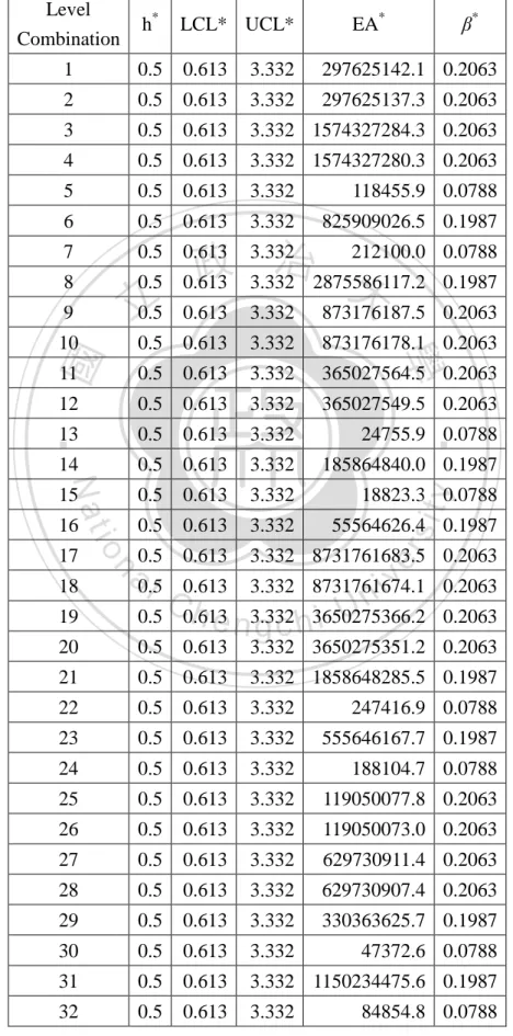
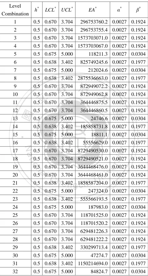
(26) Table 2-5 shows the optimal solutions for these 32 combinations of 10 parameters that we set n = 4,   0.0027 , aI  2 , and bI  2 . Table 2- 5. Optimal Solutions for Each Level Combination Level Combination. h*. LCL* UCL*. 1. 0.5. 0.613. 3.332. 297625142.1 0.2063. 2. 0.5. 0.613. 3.332. 297625137.3 0.2063. 3. 0.5. 0.613. 3.332 1574327284.3 0.2063. 4. 0.5. 0.613. 3.332 1574327280.3 0.2063. 5. 0.5. 0.613. 3.332. 118455.9 0.0788. 6. 0.5. 0.613. 3.332. 825909026.5 0.1987. 7. 0.5. 0.613. 8. 0.5. 9. 0.5 立. 10. EA*. β*. 3.332 212100.0 治政 0.613 3.332 2875586117.2 大. 0.0788 0.1987. 873176187.5 0.2063. 0.5. 0.613. 3.332. 873176178.1 0.2063. 11. 0.5. 0.613. 3.332. 365027564.5 0.2063. 12. 0.5. 0.613. 3.332. 365027549.5 0.2063. 13. 0.5. 0.613. 3.332. 24755.9 0.0788. 14. 0.5. 0.613. 3.332. 185864840.0 0.1987. 15. 0.5. 0.613. 3.332. 18823.3 0.0788. 16. 0.5. 0.613. 3.332. 55564626.4 0.1987. 0.5. 0.613. 3.332 8731761683.5 0.2063. 0.613. 3.332 8731761674.1 0.2063. 0.5. 20. 0.5. 21. n. 19. y. sit. io. 18. a0.5 l. er. Nat. 17. ‧. ‧ 國. 3.332. 學. 0.613. i n U. v. C0.613 h e n3.332 i g c h3650275366.2. 0.2063. 0.613. 3.332 3650275351.2 0.2063. 0.5. 0.613. 3.332 1858648285.5 0.1987. 22. 0.5. 0.613. 3.332. 247416.9 0.0788. 23. 0.5. 0.613. 3.332. 555646167.7 0.1987. 24. 0.5. 0.613. 3.332. 188104.7 0.0788. 25. 0.5. 0.613. 3.332. 119050077.8 0.2063. 26. 0.5. 0.613. 3.332. 119050073.0 0.2063. 27. 0.5. 0.613. 3.332. 629730911.4 0.2063. 28. 0.5. 0.613. 3.332. 629730907.4 0.2063. 29. 0.5. 0.613. 3.332. 330363625.7 0.1987. 30. 0.5. 0.613. 3.332. 47372.6 0.0788. 31. 0.5. 0.613. 3.332 1150234475.6 0.1987. 32. 0.5. 0.613. 3.332 17. 84854.8 0.0788.

(27) Based on the results presented in Table 2-5, we learn the following things: (1) All parameters are not significant to the optimal sampling interval h*. The value of h* is equal to the lower bound of its range, 0.5, for all levels of combinations. (2) All parameters are not significant to the optimal control limits, UCL* and LCL*. This is because in the data analysis in Table 2-5, we set aI  2 , bI  2 , and   0.0027 , it’s all the same in all 32 level combinations. We consider the parameter as significant to EA* if the difference of the average of EA* between two (or three) levels is greater than 109 (See Table 2-6.).With this criterion, Table 2-6 shows that k, Rn, λ, T1  T2 , and (1 , 2 ) are the significant parameters, and it comes the. 立. following findings:. 政治大. ‧ 國. the expected cycle cost per unit item, EA*, will increase.. 學. (1) A larger k indicates a larger EA*; because if the quality loss per unit item increases, then. ‧. (2) A larger Rn indicates a larger EA*; because if the number of products per unit time, Rn,. sit. y. Nat. increases under the expected quality cost per unit item fixed, then the expected cycle. io. er. cost, EC, will increase. Thus, EA* increases when Rn increases.. (3) When  increases, the average of EA* increases. This is because the expected time for. n. al. Ch. 1  the out-of-control period,  ET   , increases if  . engchi. iv n  Uincreases. It leads the expected. 1  quality cost for the out-of-control period ( RnlO  ET   ) to increase.   (4) When T1  T2 increases, the average of EA* increases. This is because the expected quality cost for out-of-control period increases if T1  T2 increases. Thus, EA* increases when T1  T2 increases. (5) When the shift of variance increases, the average of EA* increases. This is because the expected quality cost for out-of-control period increases if the shift of variance increases. 18.

(28) Table 2- 6. The Values of EA* for Each Parameter. k level1. . Rn. 635225692 2164033412. level2. 1884818522. T1  T2. e. 493604365 1452778121. c. 664488279 1001393972. 356010801 2026439849 1067266093 1855555935 1518650242. difference 1249592830 1808022611 1532835484 d. W. 385512028 1191067656. 517256270. (1 ,2 ). Y. level1. 1499763978 1258515057 1122735488 2030121773. level2. 1020280235 1261529157 1397308725. level3. 117735.5 979727146. difference. 479483743. 3014100. 274573237 2030004038. 政治大 We summarize the above立 data analysis in Table 2-7. In Table 2-7, if the parameter is. ‧ 國. 學. significant to optimal design parameter and they have a positive linear relationship, we use + ”. If the parameter is significant to optimal design parameter but we cannot the notation “○. ‧. define their relationship, we use the notation “Q”. If parameter is not significant, we use the. al. er. io. sit. y. Nat. notation “×”.. v. n. Table 2- 7. The Significant Parameters and Their Relationship of Each Design Parameter and EA Optimal Design parameter and EA. Ch. engchi. i n U. Parameters. k. Rn. . e. T1  T2. c. d. W. Y. (1 ,2 ). h. ×. ×. ×. ×. ×. ×. ×. ×. ×. ×. UCL. ×. ×. ×. ×. ×. ×. ×. ×. ×. ×. LCL. ×. ×. ×. ×. ×. ×. ×. ×. ×. ×. EA. + ○. + ○. + ○. ×. + ○. ×. ×. ×. ×. Q. . ×. ×. ×. ×. ×. ×. ×. ×. ×. ×. 19.

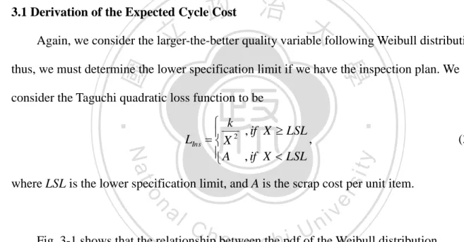
(29) CHAPTER 3. DESIGN OF ECONOMIC X CHART AND INSPECTION SPECIFICATION LIMIT FOR A PROCESS WITH WEIBULL DATA. According to the data analysis performed in Section 2.8, we find that EA* is very large in all 32 level combinations and varies extremely between each combination (104~109). So, we consider adding specification limits in order to improve the outgoing quality and reduce the expected cycle cost per unit item. To obtain the expected cost per unit time, we have to derive the expected cycle time and the expected cycle cost. The expected cycle time is the same as Equation (2-14).. 政治大. 3.1 Derivation of the Expected Cycle Cost. 立. Again, we consider the larger-the-better quality variable following Weibull distribution;. ‧ 國. 學. thus, we must determine the lower specification limit if we have the inspection plan. We consider the Taguchi quadratic loss function to be. ‧ y. (3-1). sit. Nat. LIns.  k , if X  LSL  ,  X2   A , if X  LSL. n. al. er. io. where LSL is the lower specification limit, and A is the scrap cost per unit item.. Ch. engchi. i n U. v. Fig. 3-1 shows that the relationship between the pdf of the Weibull distribution, Taguchi’s quadratic loss function, scrap cost per unit item, and the lower specification limit.. Figure 3- 1. The Weibull Distribution and Taguchi’s Quadratic Loss Function With Inspection Specification Limit 20.

(30) The expected cost can be divided into five parts; three of them are the same as we showed in Section 2.6. The expected sampling and testing cost per cycle time is the same as Equation (2-19), the cost of investigating false alarms per cycle time is the same as Equation (2-20), and the cost to locate and repair the assignable cause is the same as Equation (2-21). The others are described as follows. (1) The expected cost per unit item using the Taguchi quadratic loss function in the in-control period if the manager decides to inspect the products includes the expected quality cost when the product meets the specification limit, the scrap cost when the product fail to conform to the specification, and the inspection cost. Thus, the expected. 政治大 k. cost per unit item in the in-control period is:. 立. LI  A. LSL. . LSL. xI2. f I ( x)dx  IC ,. where IC is the inspection cost per unit item.. 學. ‧ 國. 0. f I ( x)dx  . ‧. In the in-control period, the expected quality cost per unit time is. sit. y. Nat. Rn LI .. io. n. al. Ch. 1 . . Rn LI. engchi U. er. Hence, the expected quality cost for the in-control period is:. v ni. (3-2). (2) The expected cost per unit item using the Taguchi quadratic loss function in the out-of-control period if the manager decides to inspect the products is:. LO  A. LSL. 0. . k f O ( x)dx  IC . LSL x 2 O. f O ( x)dx  . In the out-of-control period, the expected quality cost per unit of time is. Rn LO . Hence, the expected quality cost for the out-of-control period is:. 1  Rn LO  ET   .  . (3-3). By combining Equations (3-2), (3-3), (2-19), (2-20), and (2-21), we obtain the expected cycle cost, which is shown in Equation (3-4): 21.

(31) EC L  Rn LI. 1 1  (c  dn)ET  (1  1 ) sT0  α   Rn LO  ET    Y W . λ λ h λh . (3-4). Hence, the expected cost per unit time is. EAL . EC L . ET. (3-5). 3.2 Determination of the Optimum Specification Limit and Design Parameters of the Economic X Control Chart The optimal specification limit h * and the optimal control limits are obtained through the following steps: Step 1. Given k, (IC, Rn),  , e, T1  T2 , c, d, W, Y, and (1 , 2 ) .. 政治大. Step 2. and Step 3. Are the same as in Section 2.7.. 立. Step 4. We determine the optimal h* and LSL* by minimizing EAL using the routine. ‧ 國. 學. “DEoptim” in the R program under the constraints 0.5  h  8 and 0.001  LSL . 3.3 Data Analysis and the Result Comparisons with and without the Inspection Plan. ‧. The same assumptions are applied in this section as in Section 2.6. We consider 9. Nat. sit. y. parameters each with two levels, and one parameter with three levels (See Table 3-1).. n. al. er. io. Because the inspection cost per unit item (IC) and the number of products produced per unit. i n U. v. time (Rn) are correlated, so these two parameters level are set together in combination. We. Ch. engchi. put these 10 parameters in each column of orthogonal array L32(231) with 32 level combinations for 10 parameters (See Table 3-2).. Table 3- 1. The Level of Each Parameter k. (IC, Rn). (1 ,2 ). . e. T1  T2. c. d. W. Y. level 1. 5. (0.05, 1000). (1.33, 2.41). 0.01. 0.05. 3. 0.5. 0.1. 500. 250. level 2. 10. (0.1, 200). (1.43, 0.25). 0.05. 0.5. 20. 5. 1. 100. 70. level 3. (-49.89,430.35). 22.

(32) Table 3- 2. Parameters for Each Level Combination Level combination. k. (IC, Rn). (1 ,2 ). 1. 5. (0.05, 1000). (1.33, 2.41). 0.01 0.05. 3. 0.5 0.1 500 250. 2. 5. (0.05, 1000). (1.33, 2.41). 0.01 0.05. 3. 0.5 0.1 100. 3. 5. (0.05, 1000). (1.33, 2.41). 0.01. 0.5. 20. 5. 1. 500 250. 4. 5. (0.05, 1000). (1.33, 2.41). 0.01. 0.5. 20. 5. 1. 100. 5. 5. (0.05, 1000). (1.43, 0.25). 0.05 0.05. 3. 5. 1. 500 250. 6. 5. (0.05, 1000). (-49.89,430.35) 0.05 0.05. 3. 5. 1. 100. 7. 5. (0.05, 1000). 8. 5. (0.05, 1000). 9. 5. (0.1, 200). 10. 5. (0.1, 200). 11. 5. (0.1, 200). (1.33, 2.41). 0.05. 12. 5. (0.1, 200). (1.33, 2.41). 0.05. 13. 5. (0.1, 200). (1.43, 0.25). 0.01 0.05. 14. 5. 15. 5. 16. 5. 17. 10. (0.05, 1000). (1.33, 2.41). 0.05 0.05. 18. 10. (0.05, 1000). (1.33, 2.41). 0.05 0.05. 19. 10. (0.05, 1000). (1.33, 2.41). 0.05. 20. 10. a (0.05, 1000) l. 21. 10. (0.05, 1000). 22. 10. (0.05, 1000). 23. 10. (0.05, 1000). 24. 10. (0.05, 1000). (1.43, 0.25). 0.01. 25. 10. (0.1, 200). 26. 10. 27. Y. 70 70 70. Nat. io. 0.5 0.1 500 250. (-49.89,430.35) 0.05. 0.5. 20. 0.5 0.1 100. 70. 20. 0.5. 1. 500. 70. 20. 0.5. 1. 100 250. 0.5. 3. 5. 0.1 500. 0.5. 3. 5. 0.1 100 250. 20. 5. 0.1 500. 20. 5. 0.1 100 250. 3. 0.5. 1. 500. 3. 0.5. 1. 100 250. y. W. 20. 20. 5. 0.1 500. 20. 5. 0.1 100 250. 治0.05 0.05 政 (1.33, 2.41) 0.05 大 0.05 (1.33, 2.41). (-49.89,430.35) 0.01 0.05 (1.43, 0.25). 0.01. 0.5. (-49.89,430.35) 0.01. 0.5. sit. (0.1, 200). d. 0.5. er. ‧ 國. (0.1, 200). c. 0.05. 學. (0.1, 200). T1  T2. e. ‧. 立. (1.43, 0.25). . 70 70 70. 3. 0.5. 1. 500. 3. 0.5. 1. 100 250. 20. 0.5. 1. 500. 20. 0.5. 1. 100 250. 0.5. 3. 5. 0.1 500. 0.5. 3. 5. 0.1 100 250. (1.33, 2.41). 0.01 0.05. 3. 5. 1. 500 250. (0.1, 200). (1.33, 2.41). 0.01 0.05. 3. 5. 1. 100. 10. (0.1, 200). (1.33, 2.41). 0.01. 0.5. 20. 0.5 0.1 500 250. 28. 10. (0.1, 200). (1.33, 2.41). 0.01. 0.5. 20. 0.5 0.1 100. 29. 10. (0.1, 200). (-49.89,430.35) 0.05 0.05. 3. 0.5 0.1 500 250. 30. 10. (0.1, 200). 3. 0.5 0.1 100. 31. 10. (0.1, 200). 32. 10. (0.1, 200). n. 0.5. 70. (1.33, 2.41) 0.05 0.5i v n Ch U (-49.89,430.35) 0.01 0.05 engchi (1.43, 0.25). 0.01 0.05. (-49.89,430.35) 0.01. (1.43, 0.25). 0.05 0.05. (-49.89,430.35) 0.05 (1.43, 0.25). 23. 0.05. 70 70 70. 70 70 70. 0.5. 20. 5. 1. 500 250. 0.5. 20. 5. 1. 100. 70.

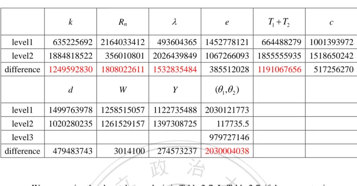
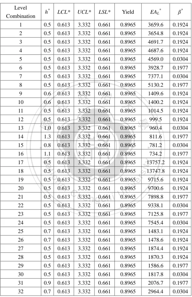
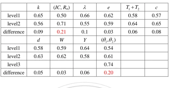
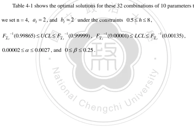
(33) Table 3-3 shows the optimal solutions for these 32 combinations of 10 parameters that we set n = 4,   0.0027 , aI  2 , and bI  2 under the constraints 0.5  h  8 and 0.001  LSL .. Based on the results presented in Table 3-3, we learn the following things: (1) All parameters are not significant to the optimal control limits, UCL* and LCL*. It’s the same reason we discussed in Section 2.8. (2) All parameters are not significant to the optimal lower specification limit, LSL*. It means that if we have the same in-control distribution, then we will obtain the same LSL*.. 立. 政治大. (3) The EA* for each level combination is much smaller than in Section 2.8. This is because. ‧ 國. 學. we adopt an inspection plan to reduce the quality cost per unit item.. ‧. We consider the parameter as significant to h* if the difference of the average of h*. y. Nat. io. sit. between two (or three) levels is greater than 0.2. Table 3-4 indicates that (IC, Rn) and. er. (1 ,2 ) are significant parameters, and it comes the following findings:. al. n. v i n C h a smaller h*; because (or smaller IC) indicates e n g c h i U if R. (1) A larger Rn. n. increases, then we must. sample more frequently in order to control the outgoing quality. (2) When the shift of variance increases, the average of h* decreases. This is because the expected quality cost for out-of-control period increases if the shift of variance increases. Then we must sample more frequently in order to detect the out-of-control of the process as soon as possible.. 24.

(34) Table 3- 3. Optimal Solutions for Each Level Combination Level Combination. h*. LCL*. UCL*. LSL*. Yield. EAL*. β*. 1. 0.5. 0.613. 3.332. 0.661. 0.8965. 3659.6. 0.1924. 2. 0.5. 0.613. 3.332. 0.661. 0.8965. 3654.8. 0.1924. 3. 0.5. 0.613. 3.332. 0.661. 0.8965. 4691.7. 0.1924. 4. 0.5. 0.613. 3.332. 0.661. 0.8965. 4687.6. 0.1924. 5. 0.5. 0.613. 3.332. 0.661. 0.8965. 4569.0. 0.0304. 6. 0.5. 0.613. 3.332. 0.661. 0.8965. 3928.7. 0.1977. 7. 0.5. 0.613. 3.332. 0.661. 0.8965. 7377.1. 0.0304. 8. 0.5. 0.613. 3.332. 0.661. 0.8965. 5130.2. 0.1977. 9. 0.6. 0.613. 1409.6. 0.1924. 10. 0.6. 0.613. 1400.2. 0.1924. 11. 0.5. 0.613. 3.332. 0.661. 0.8965. 1014.5. 0.1924. 12. 0.5. 0.613. 3.332. 0.661. 0.8965. 999.5. 0.1924. 1.0. 0.613. 3.332. 0.661. 0.8965. 960.4. 0.0304. 1.3. 0.613. 3.332. 0.661. 0.8965. 811.6. 0.1977. 0.8. 0.613. 3.332. 0.661. 0.8965. 1.1. 0.613. 3.332. 0.661. 0.8965. 0.5. 3.332. 0.661. 0.8965. 18. Nat. 0.613. 0.5. 0.613. 3.332. 0.661. 0.8965. 19. 0.5. 0.613. 3.332. 0.661. 0.8965. 20. 0.5. 21. 0.5. 22. 0.5. 23. 0.0304. 13757.2. y. 0.1924. 13747.8. 0.1924. a l 3.332 0.661 0.8965i v 0.613 n C 3.332 0.661 U 0.613 h 0.8965 engchi. 9715.6. 0.1924. 9700.6. 0.1924. 7898.8. 0.1977. 0.613. 3.332. 0.661. 0.8965. 9338.1. 0.0304. 0.5. 0.613. 3.332. 0.661. 0.8965. 7125.8. 0.1977. 24. 0.5. 0.613. 3.332. 0.661. 0.8965. 7545.4. 0.0304. 25. 0.7. 0.613. 3.332. 0.661. 0.8965. 1483.1. 0.1924. 26. 0.7. 0.613. 3.332. 0.661. 0.8965. 1478.6. 0.1924. 27. 0.5. 0.613. 3.332. 0.661. 0.8965. 1874.4. 0.1924. 28. 0.5. 0.613. 3.332. 0.661. 0.8965. 1870.3. 0.1924. 29. 0.5. 0.613. 3.332. 0.661. 0.8965. 1586.6. 0.1977. 30. 0.5. 0.613. 3.332. 0.661. 0.8965. 1817.8. 0.0304. 31. 0.9. 0.613. 3.332. 0.661. 0.8965. 2076.7. 0.1977. 32. 0.7. 0.613. 3.332. 0.661. 0.8965. 2964.4. 0.0304. 17. n. 25. 781.2 734.2. 0.1977. sit. 16. er. 15. io. ‧. ‧ 國. 14. 學. 13. 立. 3.332 0.661 治 0.8965 政 3.332 0.661 0.8965 大.

(35) Table 3- 4. The Values of h * for Each Parameter. k. (IC, Rn). level1. 0.65. 0.50. level2. 0.56. 0.71. difference. 0.09. 0.21. d. W. level1. 0.58. 0.59. level2. 0.63. 0.62.  0.66 0.55 0.1 Y 0.64 0.58. e. T1  T2. c. 0.62. 0.58. 0.57. 0.59. 0.64. 0.65. 0.03 (1 , 2 ). 0.06. 0.08. 0.54 0.61. level3 difference. 0.74 0.05. 0.03. 0.06. 0.20. 治政大this criterion, Table 3-5 shows EA * between two (or three) levels is greater than 10 . With 立 We consider the parameter as significant to EAL* if the difference of the average of 3. L. findings:. ‧. ‧ 國. 學. that k, (IC, Rn),  , T1  T2 , and (1 , 2 ) are significant, and it comes the following. (1) A larger k indicates a larger EAL*.. sit. y. Nat. (2) A larger Rn (or smaller IC) indicates a larger EAL*.. al. er. io. (3) A larger  indicates a larger EAL*.. n. (4) A larger T1  T2 indicates a larger EAL*.. Ch. engchi. i n U. v. (5) When the shift of variance increases, the average of EAL* increases. (6) All above results and reasons are the same as we discussed in Section 2.8. Table 3- 5. The Values of EA L * for Each Parameter k. (IC, Rn). level1. 2863.1. 7283.0. level2. 5873.8. 1454.0. difference. 3010.7. 5829.0. d. W. level1. 4558.3. 4373.8. level2. 4178.6. 4363.1.  3662.2 5074.7 1412.5 Y 4474.7 4262.2. level3 difference. e. T1  T2. c. 4468.9. 3737.2. 4246.8. 4268.1. 4999.8. 4490.2. 200.8 (1 , 2 ). 1262.6. 243.3. 4696.6 4419.2 3661.6. 379.7. 10.7. 212.5 26. 1035.0.

(36) We compare the data analysis of the economic X control chart for products without inspection plan with the economic X control chart for products with inspection plan (See Table 3-6). In Table 3-6, if the optimal design parameter or EA of the economic X control chart without inspection plan is greater (smaller) than the economic X control chart with inspection plan, we use the notation “↑” (“↓”). Otherwise, we use the notation “—”.. Table 3- 6. Economic X Chart for Products Without Inspection Plan Compares to Economic X Chart for Products With Inspection Plan. EAL* ↑. —. Width of control limits. —. α. — —. io. n. al. er. β*. ‧. —. 學. LCL*. Nat. ‧ 國. UCL*. y. 立. h*. 4(fixed) 政治大 ↓. sit. n. i n U. v. According to the result shown in Table 3-6, UCL*, LCL*, and β* are all the same,. Ch. engchi. regardless of whether the producer inspects the products. However, the expected cycle cost of the economic X control chart without inspection plan is greater than the expected cost of the economic X control chart with inspection plan. This result seems not reasonable. However, because the value of the coefficient of the Taguchi’s loss function (k) we set is very small. If k becomes larger, the result will reverse. It means k affects the decision making significantly. So, the producer should be careful in estimating k. In our data analysis, we suggest that the producer inspects products using LSL*  0.661 and the economic X control chart in which UCL*  3.332 and LCL*  0.613 , as well as take a sample of four samples every 0.5 units of time to obtain a lower cost of 3659.6 per unit of time. 27.

(37) We summarize the data analysis in Chapter 3 to Table 3-7. In Table 3-7, we use the same notation as we introduced in Table 2-5.. Table 3- 7. The Significant Parameters and Their Relationship of Each Design Parameter and EAL Optimal Design parameter and EAL. Parameters. ×. UCL. ×. ×. LCL. ×. ×. LSL EA L. × + ○. × + ○. . ×. 立. ×.  × × × × + ○. e. T1  T2. c. d. W. Y. (1 ,  2 ). ×. ×. ×. ×. ×. ×. Q. ×. ×. ×. ×. ×. ×. ×. ×. ×. ×. ×. ×. ×. ×. ×. ×. ×. ×. Q. ×. ×. ×. 政× 治× 大× × × ×. ×. ×. + ○. ×. ×. ×. ×. 學. h. (IC, Rn) + ○. ×. ‧. ‧ 國. k. Here, we provide an example to illustrate the determination of the optimal design. sit. y. Nat. io. er. parameters of the economic X control chart and the optimal lower specification limit and its applications. We first explain the data we used, and then construct the economic X. n. al. control chart and inspection plan. 3.4 An Example. Ch. engchi. i n U. v. 3.4.1 Data We used data from Erto, Pallotta and Park (2008). These data pertain to the breaking stress of carbon fibers: 10 samples of size n = 5 under an in-control state. We constructed the economic X control chart for sample size n = 4; however, the data provided from the article were intended for a sample size of n = 5. For our purposes, we moved the #1-#4 data in the last column (Column 5) to the #11 sample, and moved the #5-#8 data in last column to the #12 sample to obtained data for 12 samples of size n = 4.. 28.

(38) Table 3- 8. Breaking Stress of Carbon Fibres. j-th sample. Stress. 1. 3.7. 2.74. 2.73. 2.5. X 2.9175. 2. 3.11. 3.27. 2.87. 1.47. 2.68. 3. 4.42. 2.41. 3.19. 3.22. 3.31. 4. 3.28. 3.09. 1.87. 3.15. 2.8475. 5. 3.75. 2.43. 2.95. 2.97. 3.025. 6. 2.96. 2.53. 2.67. 2.93. 2.7725. 7. 3.39. 2.81. 4.2. 3.33. 3.4325. 8. 3.31. 3.31. 2.85. 2.56. 3.0075. 9. 3.15. 2.35. 2.55. 2.59. 2.66. 10. 2.81. 2.77. 2.17. 2.83. 2.645. 11. 3.6. 3.11. 1.69. 4.9. 3.325. 3.39 政 3.22 治 2.55 3.56 大立. 12. 3.18. ‧ 國. 學. 3.4.2 Estimating the in-control parameters of the Weibull distribution We calculate the maximum likelihood estimators (MLEs) of the Weibull (aI , bI ). ‧. sit. y. Nat. distribution aÎ  4.895 and bÎ  3.235 by using the routine “mle” in the R program. In ^. n. al. er. io. addition, we obtain E ( X I )  bÎ (1  1 / aˆ I )  2.966 (from Equation 2-1) and ^. i n U. v. 2 Var ( X I )  bÎ ((1  2 / aˆ I )  ((1  1 / aˆ I )) 2 )  0.480 (from Equation 2-2). We then perform a. Ch. engchi. hypothesis test and draw the Weibull probability plot for checking whether the data is following Weibull (4.895,3.235) or not.. H 0 : data is sampling from Weibull (4.895,3.235) v.s. H1 : data is not sampling from Weibull (4.895,3.235) We use the Kolmogorov-Smirnov test (K-S test) and obtain the p-value=0.3176. Because the p-value is 0.3176 is larger than   0.05 , so we do not reject the null hypothesis. That means we do not reject that the data in table 3-8 is following. Weibull (4.895,3.235) . Secondly, Fig. 3-2 shows the Weibull probability plot for the sample data in Table 3-8. 29.

(39) We can find that the p-value is greater than 0.250, so we do not reject that the data is following Weibull (4.895,3.235) .. 政治大. Figure 3- 2. The Probability Plot for Weibull Distribution. 立. 3.4.3 Simulation Data for Out-of-control Distribution. ‧ 國. 學. The simulated data from the out-of-control Weibull distribution was ( a  0.9, b  0.726 ) and 10 samples of a size of n = 4. The out-of-control mean = 0.764 and variance = 0.723.. ‧. Nat. al. 3.03. 0.23. 1.04. 1.14 C h0.27 e n g c h0.04i U 0.33. 14. 1.98. 15. 0.53. 16. 0.07. 0.12. 17. 1.95. 18. sit er. Simulated data. n. 13. io. j-th sample. y. Table 3- 9. Simulated Data From Out-of-Control Distribution. 0.09. v n i 0.58. X 1.10 0.99. 0.05. 0.24. 1.26. 0.07. 0.38. 0.47. 0.45. 0.82. 0.92. 0.18. 0.84. 0.57. 0.09. 0.42. 19. 2.85. 0.71. 1.15. 0.40. 1.28. 20. 0.08. 0.26. 1.06. 0.66. 0.52. 21. 0.39. 0.02. 2.94. 0.29. 0.91. 22. 0.03. 0.56. 2.27. 0.70. 0.89. According to our discussion in Section 3.4, we find that the expected cost per unit time for the economic X control chart with inspection plan is much smaller than the expected 30.

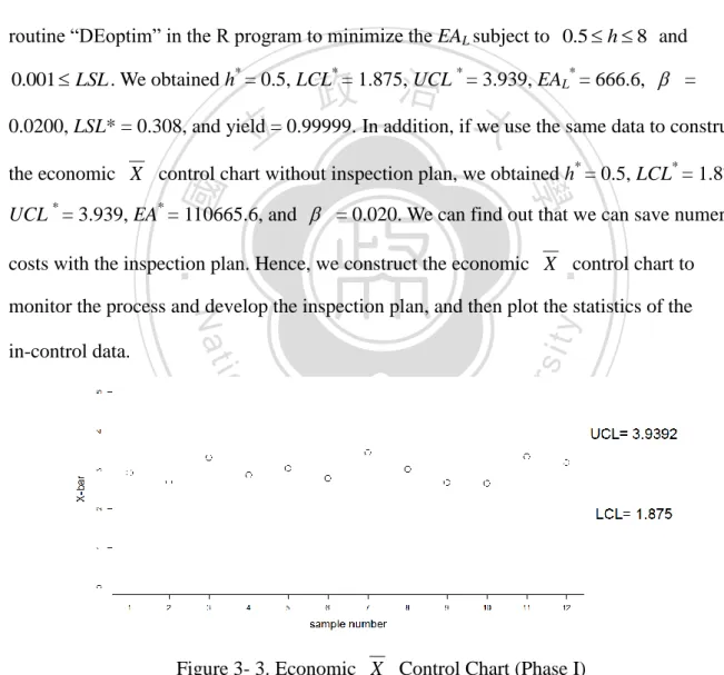
(40) cycle cost per unit time for the economic X control chart without inspection plan. So, we show how to determine the design parameters and the optimal lower specification limit simultaneously to obtain the minimal expected cost per unit time. 3.4.4 Constructing the economic X control chart and inspection plan We use the same assumptions as those presented in Section 2.6. Let n = 4, A = 20, IC = 0.05, Rn = 1,000,   0.01 , e = 0.05, T1  T2 = 3, c = 0.5, d = 0.1, W = 500, Y = 250, aˆ  4.895, bˆ  3.235 , (ˆ1,ˆ2 )  (3.179, 1.227) , and   0.0027 . Using the routine “DEoptim” in the R program to minimize the EAL subject to 0.5  h  8 and. 政治大 0.0200, LSL* = 0.308, and yield = 0.99999. In addition, if we use the same data to construct 立 0.001  LSL . We obtained h* = 0.5, LCL* = 1.875, UCL * = 3.939, EAL* = 666.6,  =. ‧ 國. 學. the economic X control chart without inspection plan, we obtained h* = 0.5, LCL* = 1.875, UCL * = 3.939, EA* = 110665.6, and  = 0.020. We can find out that we can save numerous. ‧. costs with the inspection plan. Hence, we construct the economic X control chart to. y. sit. io. n. al. er. in-control data.. Nat. monitor the process and develop the inspection plan, and then plot the statistics of the. Ch. engchi. i n U. v. Figure 3- 3. Economic X Control Chart (Phase I). Figure 3-3 shows that no points are out of the control limits for the in-control state (i.e., no false alarms occurred in Phase I). We then plotted the statistics of the out-of-control data as in Fig. 3-4. 31.

(41) Figure 3- 4. Economic X Control Chart (Phase II). 政治大 No. 13. All out-of-control data were detected. 立. Figure 3-4 shows that No.13 to 22 are out of control limits, and the first true alarm is. ‧. ‧ 國. 學. n. er. io. sit. y. Nat. al. Ch. engchi. i n U. v. Figure 3- 5. The Relationship Between the In-control and Out-of-control Distribution and the Lower Specification Limit. According to Fig. 3-5, we can find the yield for in-control state is 0.9999, and the yield for out-of-control state is 0.6299. Hence, we can improve the outgoing quality by conducting inspection, and detect the out-of-control state by monitoring the process using economic X control chart.. 32.