資產模型建構與其資產配置之應用 - 政大學術集成
139
0
0
全文
(2) 謝辭. 兩年的研究所過得真快,首先要感謝的是我的指導教授黃泓智老師,感謝黃 泓智老師在這兩年中給了我很多學術和實務上的指導,也跟著老師一起完成許多 的國科會研究案,我也從中學習到許多經驗,讓我在研究所兩年過得很充實。此 外,我也要特別感謝王昭文老師,王昭文老師對於我論文中模型選取與建構,給 了我很多的想法與指導,學習到了許多不同的模型。最後也要感謝楊曉文老師於 口試時提出許多的建議,讓我的論文可以更佳完整與豐富。. 立. 政 治 大. 研究所兩年當中,認識了許多同學,特別是精算組的夥伴們,總是讓其他組. ‧ 國. 學. 的同學羨慕我們感情如此的好,雖然研究所只有短短的兩年,但是我們的情誼是 一輩子的,最後祝福精算組的夥伴們在自己的領域追求屬於自己的目標與理想。. ‧ y. Nat. io. sit. 最後要感謝的是我的家人,總是無怨無悔的付出與陪伴,讓我可以安心的追. n. al. er. 求我自己的理想與目標,衷心的感謝我們家人,我愛你們。謹將此文獻給最摯愛 的你們。. Ch. engchi. i Un. v. 陳炫羽. 謹致於. 國立政治大學風險管理與保險學研究所 中華民國一百零二年七月. a.
(3) 摘要. 因為股票市場常具有厚尾、偏態和峰態的特性且在國際的股票市場之間,股 票報酬長存在有尾端相依的情況,所以我們的資產模型不能選用 Gaussian 分配。 近幾年來,常用 GH 分配建構單維度的股票報酬。這篇文章將利用多元仿射 JD、 多元仿射 VG 和多元仿射 NIG 分配去建構風險性資產的報酬並請應用到資產配 置。. 政 治 大. 建構風險性資產的報酬後,我們提供兩種不同形式的投資組合並且可以導出. 立. 投資組合的期望值、變異數、偏態和峰態。我們嘗試以投資組合的期望值、變異. ‧ 國. 學. 數、偏態和峰態當成我們的目標函數,然後得出未來最佳的投資組合的權重。為 了讓我們的資產配置更加動態和有效率,我們重新估計模型的參數、選擇最佳的. ‧. 投資組合權重,然後重新評估最佳的資產配置在每個決策日期。實證結果發現當. y. Nat. io. sit. 股票市場的表現好的時候,我們建議資產配置應使用偏態當成我們的目標函數,. n. al. er. 但是當股票市場的表現太好的時候,我們建議資產配置應使用變異數當成我們的 目標函數。. Ch. engchi. i Un. v. 關鍵字:厚尾、偏態、峰態、多元仿射 JD、多元仿射 VG、多元仿射 NIG、資產 配置. b.
(4) Abstract. Since the stock markets always have the characteristics of heavy-tailness, skewness and kurtosis and there exists tail dependence among the international stock markets, we can’t use the Gaussian distribution as our model. Recently, the generalized hyperbolic (GH) distribution has been suggested to fit the single stock returns. This article will use the multivariate affine JD (MAJD), multivariate affine variance gamma (MAVG) and multivariate affine normal inverse Gaussian (MANIG). 政 治 大. distributions to construct the risky asset returns, and apply them to asset allocation.. 立. ‧ 國. 學. After constructing the risky asset returns, we provide two different forms of portfolio and obtain the mean, variance, skewness, kurtosis of portfolio. We can try to. ‧. select the optimal weights of portfolio by using the mean, variance, skewness,. y. Nat. io. sit. kurtosis of portfolios as our objective functions. To make our asset allocation more. n. al. er. dynamic and efficient, we re-estimate all parameters for our models, select the. Ch. i Un. v. optimal weights of portfolio, and re-assess the optimal asset allocation at each. engchi. decision date. Empirically, when the performances of stock markets are good, we suggest that our asset allocation uses the skewness as the objective function. When the performances of stock markets are not good, we suggest that our asset allocation uses the variance as the objective function.. Key word: heavy-tailness, skewness, kurtosis, multivariate affine JD, multivariate affine variance gamma, multivariate affine normal inverse Gaussian, asset allocation. c.
(5) Catalog Catalog ............................................................................................................................ I List of Table .................................................................................................................. III List of Figure..................................................................................................................V l. Introduction ................................................................................................................. 1 2. The JD, VG and NIG Distributions ........................................................................... 5 2.1 Introductions of the JD, VG and NIG Distributions ........................................ 5. 政 治 大. 2.1.1 Introduction of the JD Distribution ...................................................... 5. 立. 2.1.2 Introduction of the VG Distribution ...................................................... 6. ‧ 國. 學. 2.1.3 Introduction of the NIG Distribution .................................................... 7 2.2 The Standardization Approaches of the JD, VG and NIG Distributions ......... 8. ‧. 2.2.1 The Standardization Approaches of the JD Distribution ...................... 8. y. Nat. io. sit. 2.2.2 The Standardization Approaches of the VG Distribution ..................... 9. n. al. er. 2.2.3 The Standardization Approaches of the NIG Distribution .................... 9. Ch. i Un. v. 2.2.4 Estimate the Parameters of the JD, VG and NIG Distribution............. 9. engchi. 3. The MAJD, MAVG and MANIG Distributions....................................................... 12 3.1 Introduction of the MAJD, MAVG and MANIG Distributions....................... 12 3.1.1 Introduction of the MAJD Distribution ............................................... 12 3.1.2 Introduction of the MAVG Distribution .............................................. 12 3.1.3 Introduction of the MAVG Distribution .............................................. 13 3.2 Estimate the parameters of the MAJD, MAVG and MANIG Distributions ... 13 3.3 MAJD, MAVG and MANIG Processes for Asset Returns .............................. 14 3.4 Portfolio selection .......................................................................................... 15 4. Empirical analysis .................................................................................................... 21 I.
(6) 4.1 The source of the data and the statistics of data ............................................ 21 4.2 Estimate the parameters of the data .............................................................. 23 4.3 The funding value for our objective functions under MAJD, MAVG and MANIG distributions............................................................................................ 24 4.3.1 The funding value on developed countries.......................................... 24 4.3.2 The funding value on developing countries ........................................ 32 4.3.3 The funding values on the assets of mixing of developed countries and developing countries .................................................................................... 40 5. Conclusion ............................................................................................................... 48. 治 政 Reference ..................................................................................................................... 49 大 立 Appendix A .................................................................................................................. 52 ‧ 國. 學. Appendix B .................................................................................................................. 54. ‧. Appendix C .................................................................................................................. 56. sit. y. Nat. Appendix D .................................................................................................................. 76. io. er. Appendix E .................................................................................................................. 95 Appendix F................................................................................................................. 107. al. n. iv n C Appendix G ................................................................................................................ 119 hengchi U. II.
(7) List of Table Table 1. Descriptive statistics of developed countries of weekly returns of stock indices ........................................................................................................ 22 Table 2. Descriptive statistics of developing countries of weekly returns of stock indices ........................................................................................................ 22 Table 3. The returns of portfolio for (P1), (P2), (P3), (P4) and (P5) on developed countries under MAJD, MAVG, and MANIG distributions ...................... 25. 政 治 大 under MAJD, MAVG, and MANIG distributions ..................................... 26 立. Table 4. The funding values for (P1), (P2), (P3), (P4) and (P5) on developed countries. ‧ 國. 學. Table 5. The returns of portfolio for (P1)’, (P2)’, (P3)’, (P4)’ and (P5)’, using the leverage (k) equal to 1, on developed countries under MAJD, MAVG, and. ‧. MANIG distributions ................................................................................. 29. sit. y. Nat. Table 6. The funding values for (P1)’, (P2)’, (P3)’, (P4)’ and (P5)’, using the leverage. n. al. er. io. (k) equal to 1, on developed countries under MAJD, MAVG, and MANIG. i Un. v. distributions................................................................................................ 30. Ch. engchi. Table 7. The returns of portfolio for (P1), (P2), (P3), (P4) and (P5) on developing countries under MAJD, MAVG, and MANIG distributions ...................... 33 Table 8. The funding values for (P1), (P2), (P3), (P4) and (P5) on developing countries under MAJD, MAVG, and MANIG distributions ...................... 34 Table 9. The returns of portfolio for (P1)’, (P2)’, (P3)’, (P4)’ and (P5)’, using the leverage (k) equal to 1, on developing countries under MAJD, MAVG, and MANIG distributions ................................................................................. 37 Table 10. The funding values for (P1)’, (P2)’, (P3)’, (P4)’ and (P5)’, using the leverage (k) equal to 1, on developing countries under MAJD, MAVG, and. III.
(8) MANIG distributions ................................................................................. 38 Table 11. The returns of portfolio for (P1), (P2), (P3), (P4) and (P5) on the mixing of developed countries and developing countries under MAJD, MAVG, and MANIG distributions ............................................................................... 41 Table 12. The funding values for (P1), (P2), (P3), (P4) and (P5) on the mixing of developed countries and developing countries under MAJD, MAVG, and MANIG distributions ............................................................................... 42 Table 13. The returns of portfolio for (P1)’, (P2)’, (P3)’, (P4)’ and (P5)’, using the leverage (k) equal to 1, on the mixing of developed countries and. 治 政 developing countries under MAJD, MAVG, 大and MANIG distributions . 45 立 Table 14. The funding values for (P1)’, (P2)’, (P3)’, (P4)’ and (P5)’, using the ‧ 國. 學. leverage (k) equal to 1, on the mixing of developed countries and. ‧. developing countries ................................................................................ 46. n. er. io. sit. y. Nat. al. Ch. engchi. IV. i Un. v.
(9) List of Figure Figure 1. The funding values for (P1), (P2), (P3), (P4) and (P5) on developed countries under MAJD, MAVG, and MANIG distributions .................... 27 Figure 2. The funding values for (P1)’, (P2)’, (P3)’, (P4)’ and (P5)’, using the leverage (k) equal to 1, on developed countries under MAJD, MAVG, and MANIG distributions ........................................................................ 31 Figure 3. The funding values for (P1), (P2), (P3), (P4) and (P5) on developing. 政 治 大 Figure 4. The funding values for (P1)’, (P2)’, (P3)’, (P4)’, and (P5)’, using the 立. countries under MAJD, MAVG, and MANIG distributions .................... 35. ‧ 國. 學. leverage (k) equal to 1, on developing countries under MAJD, MAVG, and MANIG distributions ........................................................................ 39. ‧. Figure 5. The funding values for (P1), (P2), (P3), (P4) and (P5) on the mixing of. Nat. sit. y. developed countries and developing countries under MAJD, MAVG, and. n. al. er. io. MANIG distributions ............................................................................... 43. i Un. v. Figure 6. The funding values for (P1)’, (P2)’, (P3)’, (P4)’ and (P5)’, using the. Ch. engchi. leverage (k) equal to 1, on the mixing of developed countries and developing countries ................................................................................ 47. V.
(10) l. Introduction In the past few decades, several financial crisis, for example U.S. stock market crash in 1987, subprime mortgage crisis in 2007, and universal stock market crash in 2008, not only caused lots of tremendous fluctuation in financial market, but also caused lots of huge losses for individual investors and many funds in stock markets. Since the finance data always have the characteristics of heavy-tailness, non-zero skewness and positive excess kurtosis and there exists tail dependence among the international finance data, we can’t suppose that the finance data adhere to the. 政 治 大. distribution of returns of portfolio, which is elliptically symmetric. For individual. 立. investors and funding managers, it is important to choose models to construct the. ‧ 國. 學. multi-asset investment model to catch those characteristics in financial data and to determine the best method for optimal asset allocation strategy.. ‧. There are many methods for optimal asset allocation strategy. The most popular. y. Nat. io. sit. optimal portfolio asset allocation is proposed with an article “Portfolio Selection” by. n. al. er. Markowitz (1952), which is the mean-variance (MV) rule. The investor has two ways. Ch. i Un. v. to determine the optimal portfolio asset allocation. First, the investor can maximize. engchi. the return of portfolio given a certain level under the variance of portfolio. Second, the investor can minimize the variance of portfolio given a certain level under the return of portfolio. However, there is controversy over the issue of whether higher moments should be considered in portfolio selection. Tobin (1958) and Chamberlain (1983) show that the mean-variance (MV) optimization is appropriate to capture the tradeoff between risk and return only if the distribution of returns of portfolio is elliptically symmetric, where multivariate normality is an special case. But the finance data always have the characteristics of heavy-tailness, non-zero skewness and positive excess kurtosis, many studies show that stock returns often are not 1.
(11) symmetrical. For example, Mandelbort (1963), Fama (1965) and Kon (1984) find that lots of returns occur more frequently than they would be under normal distribution. Beedles (1979) finds that the American stock returns are skewed, even though he finds measure of skewness quite unstable over the time. Simkowitz and Beedles (1980) find that individual stock returns are positively skewed. Beedles (1986) finds that the Australian stock returns are significant positive skewness. Aggarwal, Rao and Hiraki (1989) find that the Japanese stock returns have significant and persistent skewness and kurtosis. Alles and Kling (1994) show that both equity and bond indices have negative skewness. Theodossiou (1988) reports skewness in international stock. 治 政 returns, foreign exchange rates, and commodity returns. 大Bekaert, Erb, Harvey and 立 Viskanta (1998) and Erb, Harvey and Viskanta (1999) find that emerging markets ‧ 國. 學. equities and bonds display skewness. In addition, Arditti (1967) and Scott and. ‧. Horvath (1980) also show that investors prefer positive skewness to negative one.. sit. y. Nat. Machina and Muller (1987) and Jurczenko and Maillet (2006) mention the higher. io. er. moments of return distributions are relevant to the investor's decision. Maroua and. al. Jean-Luc (2010) use the international portfolio optimization with higher Moments.. n. iv n C Therefore, we can’t neglect the skewness kurtosis of stock returns. h e nand gchi U. Since the finance data always have the characteristics of heavy-tailness, non-zero skewness and positive excess kurtosis and there exists tail dependence between the international finance data, we can’t use the Gaussian distribution as our model. Therefore, Barndorff-Nielsen (1977) introduced the generalized hyperbolic (GH) distributions and first applied them to model grain size distributions of wind blown sands and the generalized hyperbolic (GH) distributions have been suggested to fit financial data. The variance gamma (VG) and normal inverse Gaussian (NIG) distributions, which were proposed by Barndorff-Nielsen(1978), are the special cases of the generalized hyperbolic (GH) distribution. In finance, Eberlein and Keller (1995) 2.
(12) use the GH distributions to fit the single assets for German, Prause (1997) also uses the GH distributions to fit the single assets for international indexes and Fajardo and Farias (2004) use the GH distributions to fit the single assets for Brazilian data. Then, multivariate generalized hyperbolic (MGH) distributions were introduced and investigated by Barndorff-Nielsen (1978) and Blasild and Jensen (1981). Prause (1999) uses MGH distributions to fit the financial market data. Unfortunately, the MGH parameter estimation procedure is computationally intense and the MGH distributions are not be capable of modeling the tail-dependence. Since the MGH distributions have some shortcomings, Multivariate affine generalized hyperbolic. 治 政 (MAGH) distributions were introduced by Schmidt et 大 al. (2006). MAGH distributions 立 can capture heavy-tailness, skewness, kurtosis, tail dependence and have a simple way ‧ 國. 學. to estimate parameters. Recently, Fajardo and Farias (2009) use the MAGH. sit. y. Nat. MAGH distributions to price multidimensional derivative.. ‧. distributions to do an empirical investigation and Fajardo and Farias (2010) use the. io. er. Although the past papers point out that the stock markets have the. al. characteristics of heavy-tailness, non-zero skewness and positive excess kurtosis,. n. iv n C many asset allocation strategies always to use mean-variance (MV) rule. In this h elike ngchi U paper, we not only consider mean-variance (MV) rule, but also consider the skewness and kurtosis of portfolios for our asset allocation strategies. Then, we provide two different forms of portfolio. For the first portfolio, we consider that our assets include the risky assets and risk-free asset. For the second one, we consider the risky asset as our assets and use the leverage of risky assets to invest. We compare the performance of funding values, using the above asset allocation strategies, under the assets of developed countries, developing countries and the mixing of the developed countries and developing countries. The assets of developed countries include the S&P500 of United States, the DAX of Germany, the CAC40 of France and the FTSE100 of 3.
(13) England. The assets of developing countries include the BSE SENSEX of India, the IBOVESPA of Brazil, the RTS of Russia and the SSE Composite Index of China. The mixing assets of developed countries and developing countries include the S&P500 of United States, the FTSE100 of England, the RTS of Russia and the SSE Composite Index of China. Using the same as Schmidt et al. (2006) and Fajardo and Farias (2010) papers to introduce the multivariate affine JD (MAJD), multivariate affine variance gamma (MAVG) and multivariate affine normal inverse Gaussian (MANIG) distributions as our asset models, we construct the risky asset returns by using the MAJD, MAVG and. 治 政 MANIG distributions to catch tail dependence in the international stock markets. 大 立 This paper is organized as the following: in section 2, we introduce the JD, VG ‧ 國. 學. and NIG distributions and estimate the parameters of the JD, VG and NIG. ‧. distributions; in section 3, we introduce the MAJD, MAVG and MANIG distributions,. sit. y. Nat. constructing the risky asset returns by using the MAJD, MAVG and MANIG. io. al. er. distributions and provide two different forms of portfolios for optimal portfolio asset. n. allocation; in section 4, we present an empirical analysis; and in the last section, we present our conclusions.. Ch. engchi. 4. i Un. v.
(14) 2. The JD, VG and NIG Distributions In this paper, we choose the MAJD, MAVG and MANIG distributions to construct our logarithm returns. Before using those distributions, we should understand the JD, VG and NIG distributions. Therefore, in this section, we introduce the JD, VG and NIG distributions, including the distribution’s probability density function, characteristic function, mean and variance. In order to estimate the parameters of the JD, VG and NIG distributions easily, we standardize the JD, VG and NIG distributions.. 政 治 大 2.1 Introductions of the JD, VG and NIG Distributions 立. ‧ 國. 學. 2.1.1 Introduction of the JD Distribution. If a random variable X follows the JD distribution, which we denote. ‧. X ~ JD( x; a, , N , N , Y ) , then. Nat. y. N. i 1. al. (2-1). er. io. sit. X a Z Yi ,. n. where Z follows standard normal distribution; N follows the Poisson distribution with intensity N ; and each. iv n C hen Y , which is independent g c h i Uof Z i. and N , follows. normal distribution with mean Y and variance Y2 . Therefore, the probability density function of the JD is . . . f JD ( x a, , N , Y , Y ) x; a N Y , 2 N Y2 N i Pr N i i 1 . i 0. Ni e i!. (2-2) N. ( x; a i Y , i ) 2. 2 Y. where ( x; , ) is a normal probability density function with mean and 2. 2. variance . 5.
(15) The characteristic function of the JD distribution is. iY 12 2Y2 1 2 2 JD ( a, , N , Y , Y ) exp ia N e 1 . 2 . (2-3). Therefore, the mean and variance of the JD distribution are. E ( X ) a N Y ,. (2-4). Var ( X ) 2 N Y2 Y2 .. (2-5). 2.1.2 Introduction of the VG Distribution. 政 治 大. The introduction of generalized hyperbolic (GH) distribution was proposed by. 立. Barndorff-Nielsen(1977), and the VG and NIG distributions, which were proposed by. ‧ 國. 學. Barndorff-Nielsen(1978), are the special cases of the generalized hyperbolic (GH) distribution. Therefore, before introducing the VG and NIG distributions, we should. ‧. first introduce the GH distribution.. y. Nat. io. sit. The generalized hyperbolic (GH) probability density function, which was. n. al. er. proposed by Prause(1999), is. fGH ( x , , , , ) . Ch. 2 2 . . . engchi. . 2 K 2 2. . e. i Un. v. K. ( x ). . 1 2. . 2 ( x )2. (x ) 2. 2. . . 1 2. (2-6). where K is the modified Bessel function of the second kind with index ; is the scale parameter; is the shift parameter; and , and determine the shape of the generalized hyperbolic (GH). If we want to obtain the VG distribution, we should let 0 , 0 and K ( x) ~ ( )2 1 x as 0 and x 0 in Equation (2-6). Therefore, if a. 6.
(16) random variable X follows the VG distribution, we denote X ~ VG( x; , , , ) . Then, the probability density function of the VG is. 2 2 x . fVG ( x , , , ) . . 2 . 1 2. . K 1 2. . 1 2. x . ( ). e ( x ). (2-7). The characteristic function of the VG distribution is . VG ( , , , ) e. i . 2 2 2 . i 2 . (2-8). Therefore, the mean and variance of the VG distribution are. 立. 2 政 治 , 大. E( X ) . 2. (2-9). 2. 2 2 2 Var ( X ) 2 1 . 2 2 2 . ‧. ‧ 國. 學. (2-10). y. Nat. 2.1.3 Introduction of the NIG Distribution. er. io. sit. If we want to obtain the NIG distribution, we should let 0.5 , K0.5 ( x) x 0.5e x and K ( x) K ( x) as 0 and x 0 in Equation (2-6). 2. n. al. Ch. engchi. i Un. v. Therefore, if a random variable X follows the NIG distribution, we denote. X ~ NIG( x; , , , ) . Then, the probability density function of the NIG is. . f NIG ( x , , , ) exp 2 2 x . . K1 2 x 2. x . 2. 2. .(2-11). The characteristic function of the NIG distribution is. NIG ( , , , ) exp i . 2. 2. Therefore, the mean and variance of the NIG distribution are. 7. . 2 2 i . . (2-12).
(17) . E( X ) . Var ( X ) . . 2 2 2 2. 2. 3/2. ,. (2-13). .. (2-14). 2.2 The Standardization Approaches of the JD, VG and NIG Distributions In this section, we want to standardize the JD, VG and NIG distributions. Then, we let. X a b Z. (2-15) 治 政 where X ~ JD,VG and NIG ; and Z is a standardized 大random variable which 立 satisfied E (Z ) 0 and Var (Z ) 1 . Therefore, after standardizing the JD, VG and. ‧ 國. 學. NIG distributions, we can easily estimate the parameters of the JD, VG and NIG. ‧. distributions.. sit. y. Nat. io. er. 2.2.1 The Standardization Approaches of the JD Distribution. al. From Equation (2-4) and (2-5), if Z follows a standardized JD distribution. n. iv n C where : i( U Z ~ stdJD( z; h) ,e n g c h , , ) , we can obtain. which is denoted as. N. N. Y. a N Y and 2 1 N (Y2 Y2 ) . Therefore, the probability density function of the stdJD is . f JD ( z N , Y , Y ) i 0. Ni e i!. N. . . ( z; N Y iY , 1 N Y2 Y2 iY2 ) (2-16). where ( z; , ) is a normal probability density function with mean and 2. 2. variance .. 8.
(18) 2.2.2 The Standardization Approaches of the VG Distribution From Equation (2-9) and (2-10), if Z follows a standardized VG distribution which is denoted as Z ~ stdVG( z; ) , where : ( , ) , we can obtain. . . 2. 2 2 2 and . Therefore, the probability density function of 2 2 2 2 2. . . the stdVG is. 2 2 z . fVG ( z , ) . . 2 . . 1 2. . K 1 2. . 1 2. z . ( ). e ( z ). (2-17). 政 治 大 2. 2 2 2 where 2 and . 2 2 2 2. 立. . . ‧ 國. 學. 2.2.3 The Standardization Approaches of the NIG Distribution. ‧. From Equation (2-13) and (2-14), if Z follows a standardized NIG. Nat. engchi. . i Un. f NIG ( z , ) exp 2 2 z where . 2 2. and. . v. . Therefore, the probability density function of. 2. the stdNIG is. er. and. 2 1.5. 2. n. 2 2. sit. a l C h. io. . . y. distribution which is denoted as Z ~ stdNIG( z; ) , where : ( , ) , we can obtain. 2. 2. . K1 2 z 2. z . 2. 2. . (2-18). 1.5. 2. .. 2.2.4 Estimate the Parameters of the JD, VG and NIG Distribution We will use the maximum likelihood method to estimate the parameters of the JD, VG and NIG distributions. The following are the maximum likelihood method. 9.
(19) Suppose there is a time series X. 1. of n independent and identically. distributed, and each X i follows: iid. X i ~ f X i (a, b2 ). (2-19). 2 where a is the mean of X and b is the variance of X ; and is the. parameter of X . Then, the joint density function and likelihood function for X are n. f X ( x1 ,. , xn ) f X i ( xi ) ,. (2-20). L( x1 ,. ,x ) f治 ( x , , x ) . 政 大. (2-21). 立. i 1. n. X. 1. n. LLF ln( L( x1 ,. n. , xn )) ln( f X i ( xi )) .. 學. ‧ 國. The log-likelihood function is. i 1. (2-22). sit. y. Nat. of X .. ‧. Then, maximizing the Equation (2-22) for parameter , we can obtain the parameter. io. n. al. Then, we have. X i a b Zi , for i 1,. Ch Zi . engchi U Xi a , for i 1, b. er. From Equation (2-15), we can let. ,n.. v ni. (2-23). ,n .. (2-24). Using the transformation of random variable and Equation (2-24), we can obtain. f X i ( xi ) f Zi (. xi a 1 ) , for i 1, b b. ,n .. (2-25). Substituting the Equation (2-25) into Equation (2-22), we can obtain. x a LLF ln f Zi i ' ln b , i 1 b n. 1. X ( X1 , X 2 ,. , Xn)' 10. (2-26).
(20) where ' is the parameter of Z 2. Then, maximizing the Equation (2-26) for parameter ' , we can obtain the parameter ' of Z . When estimating the parameters of the JD, VG and NIG distributions, we can standardize the JD, VG and NIG distributions into the stdJD, stdVG and stdNIG distributions. It is a good advantage for reducing the number of estimated parameters. For example, assuming the logarithm returns follow the JD distribution, we should estimate five parameters a, , N , Y , Y . If we standardize the JD distribution, we. 政 治 大. only estimate three parameters N , Y , Y .. 立. ‧. ‧ 國. 學. n. er. io. sit. y. Nat. al. 2. Z (Z1 ,. Ch. engchi. , Zn ) ' 11. i Un. v.
(21) 3. The MAJD, MAVG and MANIG Distributions In this section, first, we introduce the MAJD, MAVG and MANIG distributions. Second, we estimate the parameters of the MAJD, MAVG and MANIG Distributions. Third, we construct the risky asset returns by using the MAJD, MAVG and MANIG distributions. Finally, we provide two different forms of portfolio to get optimal portfolio asset allocation.. 3.1 Introduction of the MAJD, MAVG and MANIG Distributions. 政 治 大 (MAGH) distributions. Because the VG and NIG are the special cases of the GH 立. Schmidt et al. (2006) introduced multivariate affine generalized hyperbolic. ‧ 國. 學. distribution, we can also define the MAVG and MANIG resembling MAGH. Before introducing the MAJD, MAVG and MANIG distributions, we let. ‧. Z (Z1 ,. , Z n ) ' be a random vector which consists of n mutually independent. y. Nat. n. al. er. io. sit. random variables with univariate standard JD, VG or NIG distributions.. Ch. 3.1.1 Introduction of the MAJD Distribution Let X ( X1 , vector M . n. engchi. i Un. v. , X n ) ' be an n -dimensional MAJD distributed with mean. and covariance matrix . nn. if X can be expressed as an affine. transformation of a vector Z : X M AZ , where A . nn. is a lower triangular. matrix such that AA ' . We denote by X ~ MAJD , , M , where the parameter vectors : (1 ,. , n ) ' and i : (Ni , Ni , Yi ) .. 3.1.2 Introduction of the MAVG Distribution Let X ( X1 ,. , X n ) ' be an n -dimensional MAVG distributed with mean. 12.
(22) vector M . n. and covariance matrix . nn. if X can be expressed as an affine nn. transformation of a vector Z : X M AZ , where A . is a lower triangular. matrix such that AA ' . We denote by X ~ MAVG , , M , where the parameter vectors : (1 ,. , n ) ' and i : (i , i ) .. 3.1.3 Introduction of the MANIG Distribution Let X ( X1 , vector M . n. , X n ) ' be an n -dimensional MANIG distributed with mean X can be expressed as an affine 政 治 if 大. and covariance matrix . 立. nn. nn. transformation of a vector Z : X M AZ , where A . is a lower triangular. ‧ 國. 學. matrix such that AA ' . We denote by X ~ MANIG , , M , where the. , n ) ' and i : (i , i ) .. ‧. parameter vectors : (1 ,. sit. y. Nat. n. al. er. io. 3.2 Estimate the parameters of the MAJD, MAVG and MANIG Distributions. i Un. v. To estimate the parameters of the MAJD, MAVG and MANIG distributions, we. Ch. engchi. use the algorithm used by Schmidt et al. (2006) and Fajardo and Farias (2009). Then, we use the following steps to estimate the parameters of the MAJD, MAVG and MANIG distributions: (1) Get Z B( X M ) , where B is the inverse Cholesky factorization of the covariance matrix of X and Z is the set of independent stdJDs, stdVGs or stdNIGs. (2) Estimate the univariate stdJDs, stdVGs or stdNIGs by using maximum likelihood estimation. (3) Translate the univariate parameters into multivariate parameters and use the. 13.
(23) Jacobian determinant, the probability density function of X can be represented as. f X ( x) A where x ( x1 ,. , xn ) ' and z ( z1 ,. 1. n. f i 1. Zi. ( zi ). (3-1). zn ) ' B( x M ) .. In addition, the characteristic function of X is. X ( ) E ei ' X ei ' M Z ( i ) , n. where 1 ,. , n ' and ' 1 ,. (3-2). i. i 1. , n ' A .. 政 治 大 3.3 MAJD, MAVG and MANIG Processes for Asset Returns 立. ‧ 國. 學. In this section, we would construct the risky asset returns by using the MAJD, MAVG and MANIG distributions. Then, we define risky asset returns and risk-free. ‧. asset return. The risky asset returns over a small time interval are defined as the. al. n where Si (t ) is the i. th. Ch. , n 1, t 1,. er. io. Ri (t ) ln(Si (t )) ln(Si (t 1)), i 1,. sit. y. Nat. following:. i Un. ,T. (3-3). v. asset price at time t . The return on the risk-free asset over. engchi. the same time interval equals rf . We construct the risky asset returns by using the MAJD, MAVG and MANIG distributions, which is presented by Fajardo and Farias (2010); that is. R1 (t ) m1 a11 0 R2 (t ) m2 a21 a22 R(t ) Rn (t ) mn an an 2. 0 Z1 Z 2 M AZ 0 ann Z n . (3-4). where mi is the mean of the asset return Ri (t ) and A is a lower triangular matrix such that the covariance matrix is equal to AA ' . According to Equation (3-2), the 14.
(24) characteristic function of the logarithm of assets returns is. R ( ) E (e. i ' R ( t ). )e. i ' M. n. i 1. Zi. ( i ) .. (3-5). 3.4 Portfolio selection After we estimated the MAJD, MAVG and MANIG parameters and constructed the risky asset returns by using the MAJD, MAVG and MANIG distributions, we mainly want to use the skewness and kurtosis of MAJD, MAVG and MANIG distributions as our objective functions. Therefore, we have to decide the form of. 政 治 大 The first portfolio and the fund invested by the weights and asset returns are 立. portfolio. The following we provide two different forms of portfolios. 1). ‧ 國. ‧. F (t 1) F (t ) 1 RP (t ) ,. (3-6) (3-7). , wn are the weights of the risky asset returns; wn 1 is the weight of the. sit. y. Nat. where w1 ,. wn Rn (t ) wn1rf ,. 學. RP (t ) w1R1 (t ) w2 R2 (t ) . n. al. er. io. risk-free asset return ( rf ); and F (t ) means the fund we hold at time t .. Ch. i Un. v. Because we mainly want to use the skewness and kurtosis of RP (t ) as our objective. engchi. functions and compare the mean and variance of RP (t ) as our objective functions to the skewness and kurtosis of RP (t ) as our objective functions for optimal portfolio asset allocation, we need to know the mean, variance, skewness and kurtosis of RP (t ) under the MAJD, MAVG and MANIG distributions. Here, we only present the mean, variance, skewness and kurtosis of RP (t ) under the MAVG distribution, and the others are provided in Appendix A. From Equation (2-8), (2-9), (2-10), (3-4), (3-5) and (3-6), we have the characteristic. 15.
(25) function of RP (t ) ; that is n. R (t ) e. it (. wk mk wn1rf ) k 1. P. .. wk 1ak 1 k wn ank ) e n k 1 k2 k2 2 [ it ( w a w a k k kk k 1 k 1 k k ( 2 2 ) i k 2 k 2 k t ( wk akk ( k k ). (3-8). ( k2 k2 )2 2 2 2( k k ) wn ank )]2 . Therefore, the mean, variance, skewness and kurtosis of RP (t ) are n. E ( RP ) wi mi wn 1rf ,. 政 治 大. (3-9). i 1. 立. n. i 1. wn ani )2 ,. Skewness( RP ) . i ii. wi 1ai 1 i . 1 2 wn ani )3 2 2 2 2 i i i i . io. al. n. Kurtosis( RP ). C h w a ) 8U n i e n g c1h i. 4 6( wi aii wi 1ai 1 i n ni i2 i2 i 1 n ( wi aii wi 1ai 1 i i 1 n. 1.5. wn ani ) 2 . ,. (3-11). er. Nat. n ( wi aii wi 1ai 1 i i 1. y. i 1. i. ‧. . . sit. n. 2 (w a. (3-10). 學. ‧ 國. Var ( RP ) (wi aii wi 1ai 1 i . v. 2 i. ( i2 i2 ). wn ani ) . . 8i4 2 2 2 ( i i ) . 2. .. (3-12). 2. 2) The second portfolio and the fund invested by the weights and asset returns are. RP (t ) w1L1R1 (t ) w2 L2 R2 (t ) . wn Ln Rn (t ) ,. F (t 1) F (t ) 1 RP (t ) ,. where w1 ,. , wn are the weights of the risky asset returns; L1 ,. (3-13) (3-14). , Ln are the. leverages of the risky asset returns; and F (t ) means the fund we hold at time t . 16.
(26) As above, we need to know the mean, variance, skewness and kurtosis of RP (t ) under the MAJD, MAVG and MANIG distributions. Here, we only present the mean, variance, skewness and kurtosis of RP (t ) under the MAVG distribution, and the others are provided in Appendix B. From Equation (2-8), (2-9), (2-10), (3-4), (3-5) and (3-13), we have the characteristic function of RP (t ) ; that is n. R (t ) e. it. wk Lk mk. . k 1. P. 政 治 大. 2. 2. ‧ 國. 立. .(3-15) 2 2 2 ( k k ) 2 2 2( k k ) wn Ln ank )]2 . 學. i k (2 k 2 k ) t ( wk Lk akk wk 1Lk 1ak 1 k wn Ln ank ) e ( k k ) n k 1 k2 k2 2 [ it ( w L a w L a k k k kk k 1 k 1 k 1 k k. n. y. Nat. E ( RP ) wi Li mi ,. io. i 1. n. al. Ch. engchi. wn Ln ani )2 ,. er. n. sit. i 1. Var ( RP ) ( wi Li aii wi 1Li 1ai 1 i Skewness( RP ). ‧. Therefore, the mean, variance, skewness and kurtosis of RP (t ) are. i Un. (3-16) (3-17). v. 1 2 3 2 2i ( wi Li aii wi 1 Li 1ai 1 i wn Ln ani ) 2 2 2 i 1 i i i i , (3-18) 1.5 n 2 ( wi Li aii wi 1 Li 1ai 1 i wn Ln ani ) i 1 n. Kurtosis( RP ) 6( wi Li aii wi 1 Li 1ai 1 i i2 i2 i 1 n. . wn Ln ani ) 4 8i2 8i4 1 ( 2 2 ) ( 2 2 )2 .(3-19) i i i i . n ( wi Li aii wi 1 Li 1ai 1 i i 1. wn Ln ani ) . 2. 2. We already have the mean, variance, skewness and kurtosis of RP (t ) under the 17.
(27) MAJD, MAVG and MANIG distributions. Then, we want to use mean, variance, skewness and kurtosis as our objective functions. Our objective functions are presented as the following: a) Maximize the mean of RP (t ) : The objective function (P1) under the first portfolio is Maximize ( P1) subject to . E ( RP ) w1 w2 0 w1 ,. wn 1 1 . , wn 1 1. The objective function (P1)’ under the second portfolio is. 立. P. 1. n. k L1 ,. , Ln k. 0 w1 ,. .. , wn 1. 學. ‧ 國. E(R ) 政 治 w 大 w 1. Maximize subject to ( P1) ' . ‧. b) Minimize the variance of RP (t ) :. E ( RP ) k. n. al. Var ( RP ). Ch. er. io. Minimize subject to ( P 2) . sit. y. Nat. The objective function (P2) under the first portfolio is. v ni. w1 w2 . wn 1 1. e n g0chw i, U, w. n 1. 1. 1. The objective function (P2)’ under the second portfolio is. Minimize subject to ( P 2) ' . Var ( RP ) w1 . wn 1. k L1 , 0 w1 ,. , Ln k , wn 1. c) Maximize the skewness of RP (t ) : The objective function (P3) under the first portfolio is. 18. .. ..
(28) Maximize subject to ( P3) . Skewness ( RP ) E ( RP ) k w1 . wn 1 1. 0 w1 ,. .. , wn 1 1. The objective function (P3)’ under the second portfolio is. Maximize subject to ( P3) ' . Skewness ( RP ) w1 . wn 1. k L1 , 0 w1 ,. .. , Ln k , wn 1. d) Minimize the kurtosis of RP (t ) :. Kurtosis ( RP ) E ( RP ) k. wn 1 1. 0 w1 ,. , wn 1 1. Nat. n. w1 w2 . Ch. k L1 ,. e n g0c wh,i 1. er. io. al. Kurtosis ( RP ). sit. The objective function (P4)’ under the second portfolio is. Minimize subject to ( P 4) ' . .. y. w1 . ‧. Minimize subject to ( P 4) . 學. ‧ 國. 治 政 The objective function (P4) under the first portfolio大 is 立. wn 1. i Un. v. , Ln k. .. , wn 1. e) Maximize (the skewness of RP (t ) - the kurtosis of RP (t ) ): The objective function (P5) under the first portfolio is. Maximize subject to ( P5) . Skewness( RP ) Kurtosis( RP ) E ( RP ) k w1 0 w1 ,. wn 1 1 , wn 1 1. The objective function (P5)’ under the second portfolio is. 19. ..
(29) Skewness( RP ) Kurtosis( RP ). Maximize subject to ( P5) ' . 立. w1 . wn 1. k L1 , 0 w1 ,. .. , Ln k , wn 1 1. 政 治 大. ‧. ‧ 國. 學. n. er. io. sit. y. Nat. al. Ch. engchi. 20. i Un. v.
(30) 4. Empirical analysis 4.1 The source of the data and the statistics of data For our asset allocation, we compare the performance of funding values, using the asset allocation strategies proposed in section 3.4, under the assets of developed countries, developing countries and the mixing of the developed countries and developing countries. The assets of developed countries include the S&P500 of United States, the DAX of Germany, the CAC40 of France and the FTSE100 of England. The assets of developing countries include the BSE SENSEX of India, the IBOVESPA of Brazil, the RTS of Russia and the SSE Composite Index of China. The. 政 治 大. mixing assets of developed countries and developing countries include the S&P500 of. 立. United States, the FTSE100 of England, the RTS of Russia and the SSE Composite. ‧ 國. 學. Index of China. For risky assets, we choose the weekly stock index data which cover. ‧. the period from January 1, 2001 to December 27, 2010 and denominate in U.S. dollars. To make our asset allocation more dynamic and efficient, we re-estimate all. y. Nat. er. io. sit. parameters for our models, select the optimal weights of portfolio, and re-assess the optimal asset allocation at each decision date. Since we want to change the weights of. n. al. Ch. i Un. v. asset allocation every three months, we choose the U.S. three-month LIBOR rates. engchi. from January 1, 2005 to December 27, 2010 as our risk-free assets. Table 1 provides the summary statistics on the returns of S&P500, DAX, CAC40 and FTSE100 from January 1, 2001 to December 26, 2005. Table 2 provides the summary statistics on the returns of BSE SENSEX, IBOVESPA, RTS and SSE Composite Index from January 1, 2001 to December 26. The summary statistics of other periods are presented in Appendix C. From Table 1, Table2 and Appendix C, we can see that all stock indices have significant non-zero skewness and positive excess kurtosis. According to the Jarque-Bera test, all P-value of stock indices are low under 0.05 level of alpha that implies the assumption of normality is rejected. 21.
(31) Table 1. Descriptive statistics of developed countries of weekly returns of stock indices Table 1 provides the summary statistics on the returns of S&P500, DAX, CAC40 and FTSE100 and its period is from January 1, 2001 to December 26, 2005. We can see S&P500 index has the lowest average weekly return and variance and DAX index has the highest average weekly return and variance. All stock indices have significant non-zero skewness and positive excess kurtosis. According to the Jarque-Bera test, all P-value of stock indices are low under 0.05 level of alpha that implies the assumption of normality is rejected.. Statistics. S&P500. DAX. CAC40. FTSE100. Mean. -0.0010. -0.0006. -0.0008. -0.0006. Median Maximum Minimum Std.Dev Skewness Kurtosis Number of data. -0.0007 0.0921 -0.1130 0.0257 -0.3596 5.3455 259. 0.0019 0.1278 -0.1361 0.0356 -0.6279 5.1931 259. 0.0009 0.0822 -0.1540 0.0305 -0.8582 6.2976 259. 0.0005 0.0690 -0.1458 0.0264 -0.7765 7.1909 259. 0.0010. 0.0010. 0.0010. 0.0010. Jarque-Bera test P-value. ‧ sit. y. Nat. Table 2.. 學. ‧ 國. 立. 政 治 大. Descriptive statistics of developing countries of weekly returns of stock indices. io. er. Table 21 provides the summary statistics on the returns of BSE SENSEX, IBOVESPA, RTS and SSE. al. n. iv n C Index has the lowest average weekly return variance and RTS hand i Uindex has the highest average weekly e h n c g return and variance. All stock indices have significant non-zero skewness and positive excess kurtosis.. Composite Index and its period is from January 1, 2001 to December 26, 2005. We can see SSE Composite. According to the Jarque-Bera test, all P-value of stock indices are low under 0.05 level of alpha that implies the assumption of normality is rejected.. Statistics. BSE SENSEX. IBOVESPA. RTS. SSE. Mean. 0.0025. 0.0014. 0.0071. -0.0030. Median Maximum Minimum Std.Dev Skewness Kurtosis Number of data. 0.0039 0.1217 -0.2234 0.0385 -1.1356 9.0415 260. 0.0084 0.1430 -0.1704 0.0589 -0.4755 3.2702 260. 0.0106 0.1162 -0.1842 0.0438 -0.4271 3.8373 260. -0.0039 0.1415 -0.1150 0.0361 0.5412 5.1626 260. Jarque-Bera test P-value. 0.0010. 0.0124. 0.0046. 0.0010. 22.
(32) 4.2 Estimate the parameters of the data Estimating the parameters of stock data under the MAJD, MAVG and MANIG distributions, we use the algorithm used by Schmidt et al. (2006) and Fajardo and Farias (2009). To make our asset allocation more dynamic and efficient, we change our asset allocation every three months and re-estimate the parameters based on the past five years data. Since we want to choose different assets to our asset allocation, we divide the estimation of parameters into three parts. First part, we use the assets of developed countries including the S&P500, DAX, CAC40 and FTSE100. Second part, we use the assets of developing countries including the BSE SENSEX, IBOVESPA,. 治 政 RTS and SSE Composite Index. Third part, we use the大 mixing assets of developed 立 countries and developing countries including the S&P500, FTSE100, RTS and SSE ‧ 國. 學. Composite Index. Under the MAJD, MAVG and MANIG distributions, the. ‧. parameters of three parts are presented in Appendix D.. n. er. io. sit. y. Nat. al. Ch. engchi. 23. i Un. v.
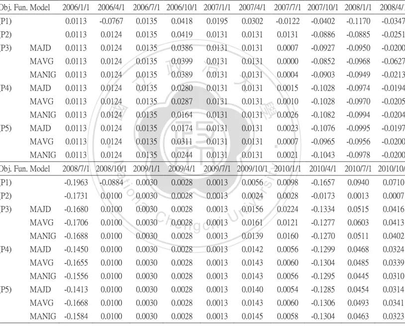
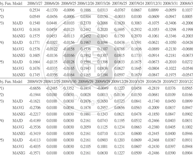
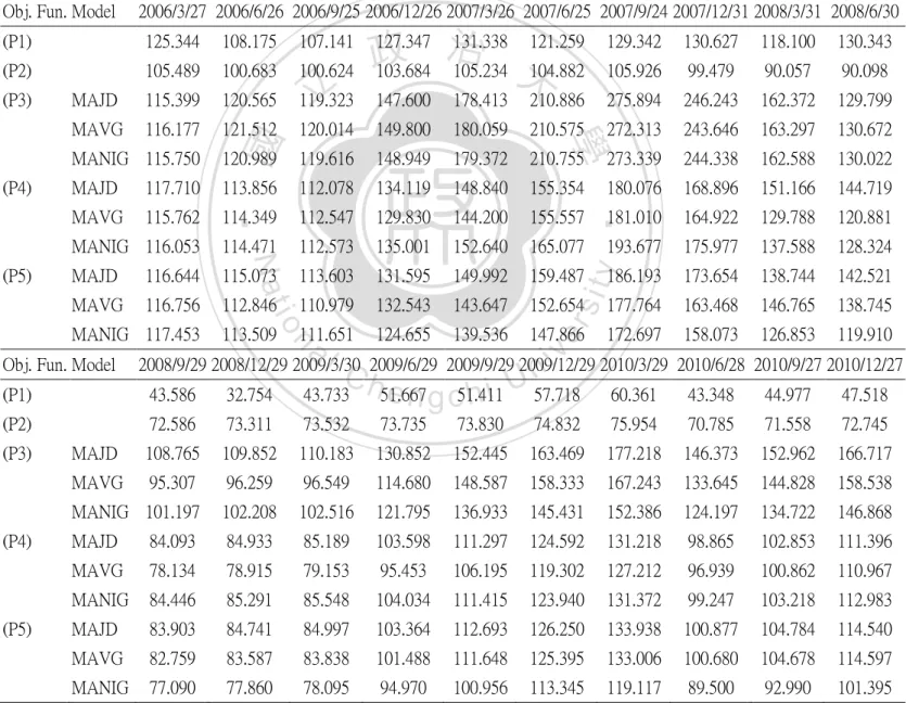
(33) 4.3 The funding value for our objective functions under MAJD, MAVG and MANIG distributions In section 4.2, we already estimated all parameters under MAJD, MAVG and MANIG distributions. We can use the mean, variance, skewness and kurtosis as objective functions under MAJD, MAVG and MANIG distributions, introduced in section 3.4, Appendix A and Appendix B, to get the optimal weights and funding value. For the constraint of (P2), (P3), (P4) and (P5), the mean of RP (t ) has to be larger than the U.S. weekly LIBOR rate at least. For the constraint of (P1)’, (P2)’,. 政 治 大 the equation (3-4), the funding values for (P1), (P2), (P1)’ and (P2)’ are the same 立. (P3)’, (P4)’ and (P5)’, we choose the leverage (k) be equal to 1, 2 or 3. According to. 4.3.1 The funding value on developed countries. Nat. sit. a) For the performance of funding value on the first portfolio:. y. ‧. ‧ 國. 學. under MAJD, MAVG and MANIG distributions.. n. al. er. io. Table 3 shows the returns of portfolio for (P1), (P2), (P3), (P4) and (P5) on. i Un. v. developed countries under MAJD, MAVG and MANIG distributions. Table 4 and. Ch. engchi. Figure 1 show the funding values for (P1), (P2), (P3), (P4) and (P5) on developed countries under MAJD, MAVG and MANIG distributions. From Table 3 and Table 4, we can see that the returns of portfolio for (P1) are the lowest during the 2008 financial crisis, so the funding value has a significant decline. However, the returns of portfolio for (P2), (P3), (P4) and (P5) are higher than for (P1) during the 2008 financial crisis, so the funding values have no significant decline. From Table 4 and Figure 1, we can see that the performance of funding value for (P2) is the best at the December 27, 2010.. 24.
(34) Table 3. The returns of portfolio for (P1), (P2), (P3), (P4) and (P5) on developed countries under MAJD, MAVG, and MANIG distributions Table 3 shows the returns of portfolio for (P1), (P2), (P3), (P4) and (P5) on developed countries under MAJD, MAVG and MANIG distributions. (P1) uses the mean of portfolio as objective function. (P2) uses the variance of portfolio as objective function. (P3) uses the skewness of portfolio as objective function. (P4) uses the kurtosis of portfolio as objective function. (P5) uses the skewness-kurtosis of portfolio as objective function.. Obj. Fun. Model. 2006/1/1 2006/4/1 2006/7/1 2006/10/1 2007/1/1 2007/4/1 2007/7/1 2007/10/1 2008/1/1 2008/4/1. (P1). 0.0113. -0.0767. 0.0135. 0.0418. 0.0195. 0.0302. -0.0122. -0.0402. -0.1170. -0.0347. (P2). 0.0113. 0.0124. 0.0135. 0.0419. 0.0131. 0.0131. 0.0131. -0.0886. -0.0885. -0.0251. MAJD. 0.0113. 0.0124. 0.0135. 0.0386. 0.0131. 0.0131. 0.0007. -0.0927. -0.0950. -0.0200. MAVG. 0.0113. 0.0124. 0.0135. 0.0000. -0.0852. -0.0968. -0.0627. MANIG. 0.0113. 0.0124. 0.0135. 0.0004. -0.0903. -0.0949. -0.0213. MAJD. 0.0113. 0.0124. 0.0135. 0.0399 0.0131 0.0131 治 政 0.0389 0.0131 大 0.0131. MAVG. 0.0113. 0.0124. MANIG. 0.0113. MAJD. 0.0113. MAVG. 0.0113. MANIG. 0.0113. 0.0280. 0.0131. 0.0131. 0.0015. -0.1028. -0.0974. -0.0194. 0.0135. 0.0287. 0.0131. 0.0131. 0.0010. -0.1028. -0.0970. -0.0205. 0.0124. 0.0135. 0.0164. 0.0131. 0.0131. 0.0026. -0.1082. -0.0994. -0.0204. 0.0124. 0.0135. 0.0174. 0.0131. 0.0131. 0.0023. -0.1076. -0.0995. -0.0197. 0.0124. 0.0135. 0.0311. 0.0131. 0.0131. 0.0007. -0.0965. -0.0956. -0.0200. 0.0124. 0.0135. 0.0244. 0.0131. 0.0131. 0.0021. -0.1043. -0.0978. -0.0200. 學. (P5). 立. ‧. Nat. y. (P4). ‧ 國. (P3). 2008/7/1 2008/10/1 2009/1/1 2009/4/1 2009/7/1 2009/10/1 2010/1/1 2010/4/1 2010/7/1 2010/10/1. (P1). -0.1963. -0.0884. (P2). -0.1731. 0.0100. MAJD. -0.1680. 0.0100. MAVG. -0.1706. 0.0100. MANIG -0.1688. 0.0100. MAJD. -0.1450. MAVG (P5). 0.0940. 0.0710. al iv 0.0030 0.0028 0.0013 0.0156 n C 0.0030 h0.0028 e n g c0.0013 h i U 0.0161. 0.0028. -0.0173. 0.0013. 0.0007. 0.0224. -0.1334. 0.0515. 0.0416. 0.0121. -0.1277. 0.0603. 0.0413. 0.0030. 0.0028. 0.0013. 0.0139. 0.0160. -0.1270. 0.0511. 0.0402. 0.0100. 0.0030. 0.0028. 0.0013. 0.0142. 0.0056. -0.1299. 0.0468. 0.0324. -0.1655. 0.0100. 0.0030. 0.0028. 0.0013. 0.0143. 0.0060. -0.1304. 0.0485. 0.0339. MANIG -0.1556. 0.0100. 0.0030. 0.0028. 0.0013. 0.0143. 0.0056. -0.1295. 0.0445. 0.0310. MAJD. -0.1413. 0.0100. 0.0030. 0.0028. 0.0013. 0.0140. 0.0054. -0.1285. 0.0454. 0.0314. MAVG. -0.1668. 0.0100. 0.0030. 0.0028. 0.0013. 0.0143. 0.0060. -0.1306. 0.0493. 0.0341. MANIG -0.1584. 0.0100. 0.0030. 0.0028. 0.0013. 0.0145. 0.0058. -0.1304. 0.0463. 0.0323. 0.0030. 0.0028. 0.0013. 0.0056. 0.0028. 0.0013. 0.0024. 25. er. -0.1657. n. (P4). 0.0098. io. (P3). 0.0030. sit. Obj. Fun. Model.
(35) Table 4. The funding values for (P1), (P2), (P3), (P4) and (P5) on developed countries under MAJD, MAVG, and MANIG distributions Table 4 shows the funding values for (P1), (P2), (P3), (P4) and (P5) on developed countries under MAJD, MAVG and MANIG distributions. (P1) uses the mean of portfolio as objective function. (P2) uses the variance of portfolio as objective function. (P3) uses the skewness of portfolio as objective function. (P4) uses the kurtosis of portfolio as objective function. (P5) uses the skewness-kurtosis of portfolio as objective function. According to the equation (3-4), the funding values for (P1) and (P2) are the same under MAJD, MAVG and MANIG distributions.. Obj. Fun. Model 2006/3/27 2006/6/26 2006/9/25 2006/12/26 2007/3/26 2007/6/25 2007/9/24 2007/12/31 2008/3/31 2008/6/30 (P1). 101.132. 93.375. 94.632. 98.591. 100.512. 103.546. 102.282. 98.168. 86.678. 83.673. (P2). 101.132. 102.390. 103.769. 108.114. 109.535. 110.973. 112.431. 102.473. 93.403. 91.064. MAJD. 101.132. 102.390. 103.769. 110.701. 100.437. 90.900. 89.082. MAVG. 101.132. 102.390. 103.769. 110.763. 101.321. 91.515. 85.780. MANIG 101.132. 102.390. 103.769. 107.777 109.193 110.626 治 110.760 政 107.907 109.325 大. MAJD. 101.132. 102.390. MAVG. 101.132. 109.226. 110.659. 110.703. 100.708. 91.147. 89.209. 103.769. 106.670. 108.071. 109.490. 109.655. 98.380. 88.800. 87.075. 102.390. 103.769. 106.743. 108.146. 109.565. 109.671. 98.399. 88.859. 87.039. MANIG 101.132. 102.390. 103.769. 105.469. 106.854. 108.257. 108.541. 96.793. 87.170. 85.390. MAJD. 101.132. 102.390. 103.769. 105.576. 106.963. 108.367. 108.617. 96.929. 87.283. 85.563. MAVG. 101.132. 102.390. 103.769. 106.995. 108.401. 109.823. 109.898. 99.298. 89.809. 88.010. MANIG 101.132. 102.390. 103.769. 106.302. 107.699. 109.112. 109.338. 97.929. 88.351. 86.587. io. 61.310. (P2). 75.305. 76.058. MAJD. 74.118. 74.859. MAVG. 71.148. 71.859. MANIG. 74.146. MAJD. (P4). (P5). 61.494. y. al iv 76.287 76.497 76.595 76.782 n C 75.084 h75.291 e n g c75.388 h i U 76.562. 62.695. 52.309. 57.226. 61.287. 76.993. 75.663. 75.759. 75.814. 78.273. 67.828. 71.320. 74.287. 72.075. 72.274. 72.367. 73.535. 74.425. 64.917. 68.829. 71.669. 74.887. 75.113. 75.320. 75.417. 76.463. 77.688. 67.822. 71.289. 74.152. 74.445. 75.190. 75.416. 75.624. 75.721. 76.798. 77.231. 67.197. 70.342. 72.623. MAVG. 72.636. 73.362. 73.583. 73.786. 73.880. 74.933. 75.382. 65.550. 68.729. 71.061. MANIG. 72.104. 72.825. 73.045. 73.246. 73.340. 74.389. 74.805. 65.115. 68.010. 70.116. MAJD. 73.469. 74.204. 74.427. 74.632. 74.728. 75.774. 76.186. 66.393. 69.409. 71.589. MAVG. 73.327. 74.060. 74.283. 74.487. 74.583. 75.648. 76.106. 66.170. 69.433. 71.800. MANIG. 72.870. 73.598. 73.820. 74.023. 74.118. 75.190. 75.624. 65.761. 68.809. 71.032. n. 67.251. 61.664. 26. 61.743. er. 2008/9/29 2008/12/29 2009/3/30 2009/6/29 2009/9/29 2009/12/29 2010/3/29 2010/6/28 2010/9/27 2010/12/27. (P1) (P3). sit. Nat. Obj. Fun. Model. ‧. (P5). 107.809. 學. (P4). 立. ‧ 國. (P3). 62.089.
(36) Figure 1. The funding values for (P1), (P2), (P3), (P4) and (P5) on developed countries under MAJD, MAVG, and MANIG distributions Figure 1 shows the funding values from table 4.. 立. 政 治 大. ‧. ‧ 國. 學. n. er. io. sit. y. Nat. al. Ch. engchi. 27. i Un. v.
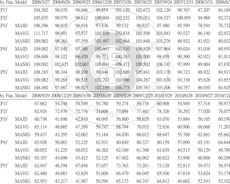
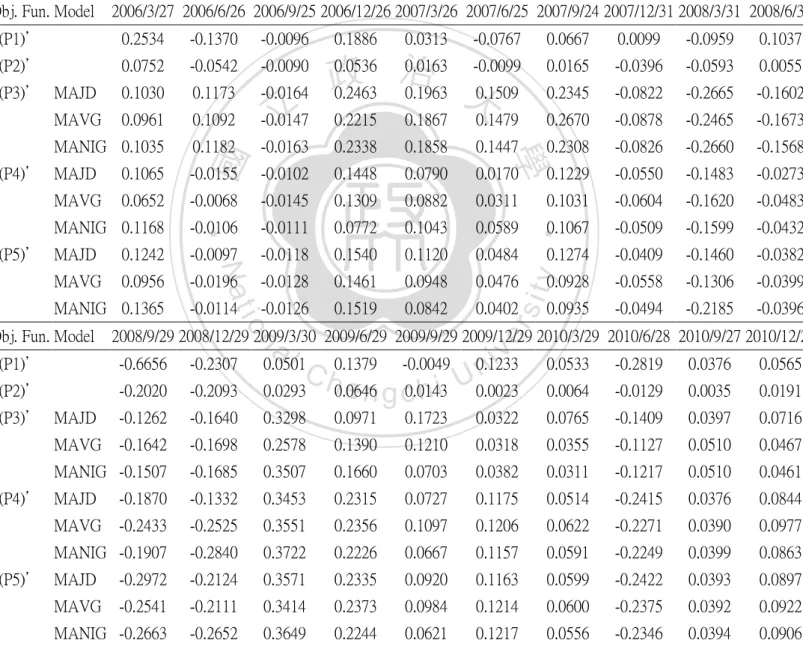
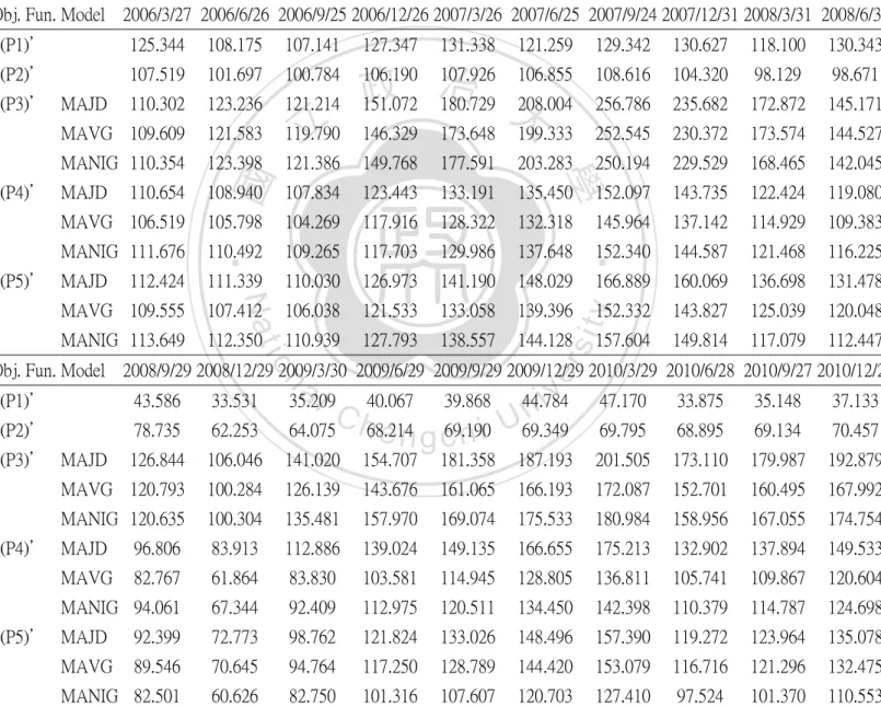
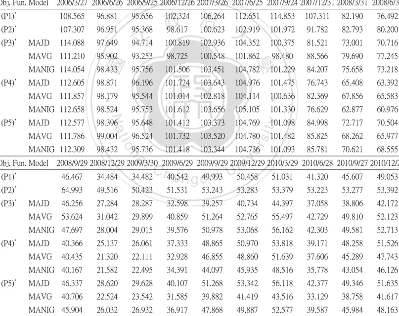
(37) b) For the performance of funding value on the second portfolio: Table 5 shows the returns of portfolio for (P1)’, (P2)’, (P3)’, (P4)’ and (P5)’, using the leverage (k) equal to 1, on developed countries under MAJD, MAVG and MANIG distributions. Table 6 and Figure 2 show the funding values for (P1)’, (P2)’, (P3)’, (P4)’ and (P5)’, using the leverage (k) equal to 1, on developed countries under MAJD, MAVG and MANIG distributions. About the returns and funding values of portfolio of leverage (k) equal to 2 and 3 are put in Appendix E. From Table 5 and Table 6, as leverage (k) equal to 1, we can see that the returns of portfolio for (P2)’ are the highest during the 2008 financial crisis, so the funding. 治 政 values have no significant decline. However, the returns 大of portfolio for (P1)’, (P3)’, 立 (P4)’, and (P5)’ are lower than for (P2)’, so the funding values have significant ‧ 國. 學. decline during the 2008 financial crisis. From Table 6 and figure 2, we can see that the. ‧. performance of funding value for (P2)’ is the best at the December 27, 2010. From. sit. y. Nat. Appendix E, we can see that when the leverage (k) is getting larger, it causes that the. io. er. returns of portfolio for (P1)’, (P2)’, (P3)’, (P4)’ and (P5) are lower than the leverage. al. (k) equal to 1’. Therefore, when the leverage (k) is getting larger, the funding values. n. iv n C have more significant decline during financial crisis. h the e n2008 gchi U. 28.
(38) Table 5. The returns of portfolio for (P1)’, (P2)’, (P3)’, (P4)’ and (P5)’, using the leverage (k) equal to 1, on developed countries under MAJD, MAVG, and MANIG distributions Table 5 shows the returns of portfolio for (P1)’, (P2)’, (P3)’, (P4)’ and (P5)’, using the leverage (k) equal to 1, on developed countries under MAJD, MAVG and MANIG distributions. (P1)’ uses the mean of portfolio as objective function. (P2)’ uses the variance of portfolio as objective function. (P3)’ uses the skewness of portfolio as objective function. (P4)’ uses the kurtosis of portfolio as objective function. (P5)’ uses the skewness-kurtosis of portfolio as objective function.. 2006/3/27 2006/6/26 2006/9/25 2006/12/26 2007/3/26 2007/6/25 2007/9/24 2007/12/31 2008/3/31 2008/6/30 0.0428. -0.0538. -0.0063. 0.0184. 0.0128. 0.0153. -0.0054. -0.0328. -0.1170. -0.0347. (P2)’. 0.0504. -0.0577. -0.0037. 0.0222. 0.0170. 0.0243. -0.0046. -0.0424. -0.0512. -0.0273. (P3)’ MAJD. 0.0640. -0.0900. -0.0196. -0.0235. -0.1219. -0.0824. -0.0231. 0.1172. -0.1094. -0.0196. 0.0307 治 0.0133 0.0070 政 0.0422 0.0116 大 0.0074. -0.0247. -0.0744. -0.0790. -0.0373. MANIG 0.0908. -0.0900. -0.0192. 0.0425. 0.0135. 0.0095. -0.0247. -0.1219. -0.0788. -0.0231. 0.0908. -0.1094. 0.0004. 0.0358. 0.0283. 0.0320. 0.0098. -0.0820. -0.0806. -0.0231. 0.0805. -0.0900. -0.0188. 0.0239. 0.0135. 0.0090. -0.0252. -0.0820. -0.0826. -0.0231. MANIG 0.0908. -0.0592. 0.0004. 0.0425. 0.0135. 0.0095. -0.0252. -0.0820. -0.0826. -0.0231. 0.0818. -0.1094. 0.0005. 0.0358. 0.0283. 0.0309. -0.0252. -0.0824. -0.0231. 0.0908. -0.0900. -0.0075. 0.0425. 0.0123. 0.0031. ‧. -0.0820. -0.0251. -0.0820. -0.0826. -0.0231. MANIG 0.0848. -0.0967. 0.0004. 0.0425. 0.0253. 0.0095. -0.0810. -0.0826. -0.0231. (P5)’ MAJD MAVG. Nat. 2008/9/29 2008/12/29 2009/3/30 2009/6/29 2009/9/29 2009/12/29 2010/3/29 2010/6/28 2010/9/27 2010/12/27. io. Obj. Fun. Model. -0.0252. sit. MAVG. (P1)’. -0.1963. -0.1909. iv 0.0048 n U. 0.0200. -0.0978. 0.0468. 0.0253. (P2)’. -0.1023. -0.1200. 0.0112. -0.0260. 0.0095. 0.0137. (P3)’ MAJD. -0.2084. -0.3135. 0.0322. 0.0759. -0.1457. 0.0423. 0.0718. -0.2148. -0.2523. -0.0285. 0.2632. 0.1514. 0.0180. 0.0400. -0.1638. 0.1274. 0.0370. MANIG -0.2573. -0.2716. -0.0285. 0.2644. 0.2039. 0.0309. 0.0399. -0.1876. 0.1272. 0.0445. -0.2587. -0.2285. 0.0268. 0.2050. 0.2847. -0.0065. -0.0021. -0.2778. 0.1261. -0.0084. -0.2587. -0.3135. -0.0285. 0.2050. 0.2882. -0.0065. -0.0021. -0.2778. 0.1261. -0.0084. MANIG -0.2587. -0.3135. -0.0285. 0.2050. 0.2882. -0.0065. -0.0021. -0.1919. 0.1261. -0.0084. -0.2587. -0.2598. 0.0269. 0.2050. 0.2793. -0.0065. -0.0021. -0.2778. 0.1261. -0.0084. -0.2533. -0.2942. -0.0285. 0.2050. 0.2882. -0.0065. -0.0016. -0.2778. 0.1261. -0.0084. MANIG -0.2587. -0.3135. -0.0285. 0.2050. 0.2882. -0.0065. -0.0021. -0.2778. 0.1260. -0.0084. (P4)’ MAJD MAVG (P5)’ MAJD MAVG. al. n. MAVG. 0.0000. 0.0006. 0.0820. er. (P4)’ MAJD. 立. ‧ 國. MAVG. 學. (P1)’. y. Obj. Fun. Model. C h0.0251 0.0334 e n g c0.1822 0.0269 0.1220 hi. -0.0027. 29. 0.0075.
(39) Table 6. The funding values for (P1)’, (P2)’, (P3)’, (P4)’ and (P5)’, using the leverage (k) equal to 1, on developed countries under MAJD, MAVG, and MANIG distributions Table 6 shows the funding values for (P1)’, (P2)’, (P3)’, (P4)’, (P5)’, using the leverage (k) equal to 1, on developed countries under MAJD, MAVG and MANIG distributions. (P1)’ uses the mean of portfolio as objective function. (P2)’ uses the variance of portfolio as objective function. (P3)’ uses the skewness of portfolio as objective function. (P4)’ uses the kurtosis of portfolio as objective function. (P5)’ uses the skewness-kurtosis of portfolio as objective function. According to the equation (3-4), the funding values for (P1)’ and (P2)’ are the same under MAJD, MAVG and MANIG distributions.. 98.670. 98.046. (P2)’. 105.035. 98.979. 98.612. (P3)’ MAJD. 106.396. 96.819. 94.918. MAVG 111.717. 99.491. 97.537. 102.120. 98.767. 87.207. 84.184. 100.804 102.522 105.011 治 政 97.836 99.132 大 99.823. 104.527. 100.095. 94.968. 92.372. 97.480. 85.599. 78.544. 76.732. 101.658. 102.834. 103.598. 101.043. 93.527. 86.140. 82.927. MANIG 109.082. 99.263. 97.359. 101.497. 102.864. 103.840. 101.276. 88.932. 81.921. 80.032. 109.082. 97.145. 97.180. 100.663. 103.510. 106.820. 107.864. 99.024. 91.038. 88.939. MAVG 108.048. 98.322. 96.470. 98.773. 100.103. 101.000. 98.459. 90.390. 82.923. 81.011. MANIG 109.082. 102.625. 102.667. 107.031. 108.472. 109.502. 106.747. 97.999. 89.904. 87.830. 108.183. 96.344. 96.390. 99.844. 102.669. 105.841. 103.178. 94.723. 86.922. 84.917. MAVG 109.082. 99.263. 98.515. 102.702. 103.966. 104.287. 101.670. 93.338. 85.628. 83.653. MANIG 108.480. 97.987. 98.023. 102.189. 104.773. 105.767. 94.757. 86.930. 84.925. (P4)’ MAJD. Nat. io. 103.106. 2008/9/29 2008/12/29 2009/3/30 2009/6/29 2009/9/29 2009/12/29 2010/3/29 2010/6/28 2010/9/27 2010/12/27. al. iv 54.780 59.274 59.716 n C 72.776 h74.606 e n g c77.094 h i U77.461. n. Obj. Fun. Model. 101.129. ‧. (P5)’ MAJD. 立. 99.854. er. 104.282. ‧ 國. (P1)’. 學. 102.672. y. 2006/3/27 2006/6/26 2006/9/25 2006/12/26 2007/3/26 2007/6/25 2007/9/24 2007/12/31 2008/3/31 2008/6/30. sit. Obj. Fun. Model. (P1)’. 67.662. 54.748. (P2)’. 82.924. 72.976. (P3)’ MAJD. 60.738. 41.696. 65.114. MANIG 59.437. 54.749. 60.908. 54.949. 57.518. 58.973. 78.326. 76.292. 77.020. 78.075. 42.819. 48.045. 56.800. 58.629. 63.076. 53.884. 56.165. 60.199. 48.685. 47.299. 59.747. 68.794. 70.032. 72.836. 60.906. 68.668. 71.207. 43.295. 42.062. 53.184. 64.030. 66.012. 68.647. 55.768. 62.861. 65.662. 65.928. 50.863. 52.225. 62.931. 80.849. 80.327. 80.159. 57.890. 65.191. 64.644. 60.052. 41.225. 40.052. 48.262. 62.169. 61.768. 61.639. 44.515. 50.129. 49.709. MANIG 65.107. 44.696. 43.423. 52.325. 67.402. 66.962. 66.822. 53.998. 60.808. 60.298. 62.947. 46.594. 47.848. 57.657. 73.763. 73.281. 73.128. 52.812. 59.473. 58.974. 62.460. 44.083. 42.829. 51.608. 66.479. 66.045. 65.936. 47.618. 53.624. 53.174. MANIG 62.953. 43.217. 41.987. 50.594. 65.173. 64.747. 64.612. 46.662. 52.543. 52.102. MAVG (P4)’ MAJD MAVG (P5)’ MAJD MAVG. 30.
(40) Figure 2. The funding values for (P1)’, (P2)’, (P3)’, (P4)’ and (P5)’, using the leverage (k) equal to 1, on developed countries under MAJD, MAVG, and MANIG distributions Figure 2 shows the funding values from table 6.. 立. 政 治 大. ‧. ‧ 國. 學. n. er. io. sit. y. Nat. al. Ch. engchi. 31. i Un. v.
(41) 4.3.2 The funding value on developing countries a) For the performance of funding value on the first portfolio: Table 7 shows the returns of portfolio for (P1), (P2), (P3), (P4) and (P5) on developing countries under MAJD, MAVG and MANIG distributions. Table 8 and Figure 3 show the funding values for (P1), (P2), (P3), (P4) and (P5) on developing countries under MAJD, MAVG and MANIG distributions. From Table 7 and Table 8, we can see that the returns of portfolio for (P3) are the highest during 2007, so the funding values have significant ascension. However, the returns of portfolio for (P1), (P3), (P4) and (P5) are lower than the return of. 治 政 portfolio for (P2) during the last half year of 2008, especially 大 the returns of portfolio 立 for (P4) and (P5) under MAVG and MANIG distributions. From Table 8 and Figure 3, ‧ 國. 學. we can see that the performance of funding values for (P3), (P4) and (P5) under. ‧. MAJD distributions are the best at the December 27, 2010, especially the performance. n. al. er. io. sit. y. Nat. of funding value for (P5) under MAJD distributions. Ch. engchi. 32. i Un. v.
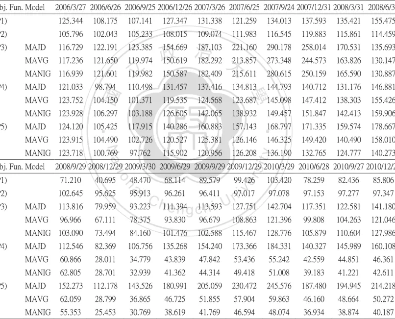
(42) Table 7. The returns of portfolio for (P1), (P2), (P3), (P4) and (P5) on developing countries under MAJD, MAVG, and MANIG distributions Table 7 shows the returns of portfolio for (P1), (P2), (P3), (P4) and (P5) on developing countries under MAJD, MAVG and MANIG distributions. (P1) uses the mean of portfolio as objective function. (P2) uses the variance of portfolio as objective function. (P3) uses the skewness of portfolio as objective function. (P4) uses the kurtosis of portfolio as objective function. (P5) uses the skewness-kurtosis of portfolio as objective function.. Obj. Fun. Model. 2006/3/27 2006/6/26 2006/9/25 2006/12/26 2007/3/26 2007/6/25 2007/9/24 2007/12/31 2008/3/31 2008/6/30. (P1). 0.2534. -0.1370. -0.0096. 0.1886. 0.0313. -0.0767. 0.1052. 0.0267. -0.0158. 0.1481. (P2). 0.0580. -0.0355. 0.0313. 0.0264. 0.0098. 0.0267. 0.0407. 0.0286. -0.0336. -0.0121. MAJD. 0.1673. 0.0468. 0.0098. 0.2535. 0.2097. 0.1820. 0.3121. -0.1108. -0.3391. -0.2043. MAVG. 0.1724. 0.0377. -0.0138. 0.2782. -0.1053. -0.3302. -0.2056. MANIG. 0.1694. 0.0399. -0.0133. 0.3015. -0.1085. -0.3381. -0.2096. MAJD. 0.2103. -0.1837. 0.1185. 0.2554 0.2103 0.1732 治 政 0.2551 0.2113 大 0.1820. MAVG. 0.2375. -0.1584. MANIG. 0.2393. MAJD. 0.1897. 0.0453. -0.0189. 0.0740. -0.0282. -0.0678. 0.1197. -0.0267. 0.1792. 0.0421. -0.0071. 0.1731. 0.0159. -0.0618. 0.1238. -0.1423. -0.0292. 0.2269. 0.1221. -0.0221. 0.0758. 0.0160. -0.0621. 0.1228. 0.2412. -0.1506. 0.1185. 0.1897. 0.1468. -0.0232. 0.0742. 0.0150. -0.0686. 0.1196. MAVG. 0.2392. -0.1568. -0.0169. 0.1733. 0.0403. 0.0061. 0.1600. 0.0212. -0.0598. 0.1247. MANIG. 0.2372. -0.1855. -0.0298. 0.1856. 0.0436. 0.0434. 0.0791. -0.0251. -0.0602. 0.1242. -0.4285. (P2). -0.1032. -0.0684. MAJD. -0.1612. -0.2975. MAVG. -0.2550. -0.3079. MANIG -0.2124. -0.2871. MAJD. -0.2338. MAVG (P5). y. 0.0402. -0.2433. 0.0534. 0.0409. al iv 0.1659 0.1949 0.0197 0.1246 n C 0.1678 h0.1972 e n g c0.0304 h i U 0.1260. 0.0006. 0.0008. 0.0013. 0.0007. 0.1170. -0.1777. 0.0446. 0.1517. 0.1151. -0.1778. 0.0446. 0.1610. 0.1451. 0.2058. 0.0110. 0.1255. 0.1153. -0.1778. 0.0446. 0.1572. -0.2681. 0.2961. 0.2671. 0.1403. 0.1240. 0.0633. -0.2387. 0.0403. 0.0967. -0.6084. -0.5398. 0.2416. 0.2605. 0.0913. 0.1169. 0.0338. -0.2296. 0.0538. 0.0337. MANIG -0.6072. -0.5430. 0.1477. 0.2557. 0.0714. 0.1152. 0.0322. -0.2318. 0.0520. 0.0337. MAJD. -0.1477. -0.2633. 0.2795. 0.2610. 0.1330. 0.1239. 0.0655. -0.2366. 0.0398. 0.0989. MAVG. -0.6072. -0.5359. 0.2801. 0.2675. 0.1098. 0.1166. 0.0338. -0.2289. 0.0542. 0.0331. MANIG -0.6054. -0.5402. 0.2088. 0.2551. 0.0816. 0.1155. 0.0318. -0.2317. 0.0525. 0.0338. 0.0030. n. (P4). 0.1911. io. -0.5420. sit. 2008/9/29 2008/12/29 2009/3/30 2009/6/29 2009/9/29 2009/12/29 2010/3/29 2010/6/28 2010/9/27 2010/12/27. (P1) (P3). ‧. Nat. Obj. Fun. Model. 學. (P5). 立. 0.4053. 0.3151. 0.1099. 0.0036. 0.0016. 0.0063. 33. er. (P4). ‧ 國. (P3).
(43) Table 8. The funding values for (P1), (P2), (P3), (P4) and (P5) on developing countries under MAJD, MAVG, and MANIG distributions Table 8 shows the funding values for (P1), (P2), (P3), (P4) and (P5) on developing countries under MAJD, MAVG and MANIG distributions. (P1) uses the mean of portfolio as objective function. (P2) uses the variance of portfolio as objective function. (P3) uses the skewness of portfolio as objective function. (P4) uses the kurtosis of portfolio as objective function. (P5) uses the skewness-kurtosis of portfolio as objective function. According to the equation (3-4), the funding values for (P1) and (P2) are the same under MAJD, MAVG and MANIG distributions.. Obj. Fun. Model. 2006/3/27 2006/6/26 2006/9/25 2006/12/26 2007/3/26 2007/6/25 2007/9/24 2007/12/31 2008/3/31 2008/6/30. (P1). 125.344. 108.175. 107.141. 127.347. 131.338. 121.259. 134.013. 137.593. 135.421. 155.475. (P2). 105.796. 102.043. 105.233. 108.015. 109.074. 111.983. 116.545. 119.883. 115.861. 114.459. MAJD. 116.729. 122.191. 123.385. 290.178. 258.014. 170.531. 135.693. MAVG. 117.236. 121.650. 119.974. 273.348. 244.573. 163.826. 130.147. MANIG 116.939. 121.601. 119.982. 154.669 187.103 221.160 治 213.857 政 150.619 182.292 大. MAJD. 121.033. 98.794. MAVG. 123.752. 182.409. 215.611. 280.615. 250.159. 165.590. 130.887. 110.498. 131.457. 137.416. 134.813. 144.793. 140.712. 131.176. 146.881. 104.150. 101.371. 119.535. 124.568. 123.687. 145.098. 147.412. 138.303. 155.426. MANIG 123.928. 106.297. 103.188. 126.605. 142.065. 138.932. 149.457. 151.847. 142.413. 159.906. MAJD. 124.120. 105.425. 117.915. 140.286. 160.883. 157.143. 168.797. 171.335. 159.574. 178.667. MAVG. 123.915. 104.490. 102.726. 120.527. 125.381. 126.146. 146.325. 149.420. 140.490. 158.010. MANIG 123.718. 100.769. 97.762. 115.902. 120.956. 126.208. 136.190. 132.765. 124.777. 140.273. io. 40.695. (P2). 102.645. 95.625. MAJD. 113.816. 79.959. MAVG. 96.966. 67.111. MANIG 103.090 MAJD. (P4). (P5). 48.470. y. al iv 95.913 96.261 96.411 97.017 n C 93.223 h111.394 e n g c113.593 h i U127.751. 103.420. 78.259. 82.436. 85.806. 97.078. 97.153. 97.277. 97.347. 142.704. 117.351. 122.581. 141.180. 78.375. 93.830. 96.679. 108.863. 121.396. 99.808. 104.263. 121.046. 73.494. 84.160. 101.476. 102.588. 115.467. 128.776. 105.879. 110.604. 127.986. 112.546. 82.369. 106.756. 135.268. 154.240. 173.366. 184.331. 140.327. 145.989. 160.108. MAVG. 60.866. 28.011. 34.779. 43.839. 47.842. 53.436. 55.242. 42.559. 44.851. 46.361. MANIG. 62.805. 28.701. 32.939. 41.362. 44.314. 49.418. 51.008. 39.183. 41.221. 42.611. MAJD. 152.273. 112.178. 143.526. 180.991. 205.059. 230.472. 245.576. 187.480. 194.945. 214.218. MAVG. 62.059. 28.799. 36.865. 46.725. 51.855. 57.904. 59.863. 46.160. 48.664. 50.272. MANIG. 55.353. 25.453. 30.769. 38.619. 41.769. 46.594. 48.074. 36.934. 38.874. 40.187. n. 71.210. 68.114. 34. 89.579. er. 2008/9/29 2008/12/29 2009/3/30 2009/6/29 2009/9/29 2009/12/29 2010/3/29 2010/6/28 2010/9/27 2010/12/27. (P1) (P3). sit. Nat. Obj. Fun. Model. ‧. (P5). 150.587. 學. (P4). 立. ‧ 國. (P3). 99.426.
(44) Figure 3. The funding values for (P1), (P2), (P3), (P4) and (P5) on developing countries under MAJD, MAVG, and MANIG distributions Figure 3 shows the funding values from table 8.. 立. 政 治 大. ‧. ‧ 國. 學. n. er. io. sit. y. Nat. al. Ch. engchi. 35. i Un. v.
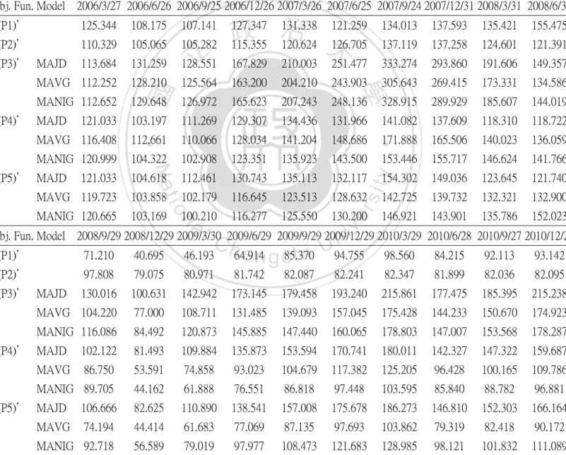
(45) b) For the performance of funding value on the second portfolio: Table 9 shows the returns of portfolio for (P1)’, (P2)’, (P3)’, (P4)’ and (P5)’, using the leverage (k) equal to 1, on developing countries under MAJD, MAVG and MANIG distributions. Table 10 and Figure 4 show the funding values for (P1)’, (P2)’, (P3)’, (P4)’ and (P5)’, using the leverage (k) equal to 1, on developing countries under MAJD, MAVG and MANIG distributions. About the returns and funding values of portfolio of leverage (k) equal to 2 and 3 are put in Appendix F. From Table 9 and Table 10, as leverage (k) equal to 1, we can see that the returns of portfolio for (P3)’ are the highest during 2007, but are the lowest during the. 治 政 first half year of 2008. From Table 10 and figure 4, we大 can see that the performance of 立 funding value for (P3)’ is the best at the December 27, 2010. From Appendix F, we ‧ 國. 學. can see that when the leverage (k) is getting larger, it causes that the returns of. ‧. portfolio for (P3)’, (P4)’ and (P5)’ are higher than the leverage (k) equal to 1 during. sit. y. Nat. 2007 and the returns of portfolio for (P3)’, (P4)’ and (P5)’ are lower than the leverage. io. er. (k) equal to 1 during 2008. Therefore, when the leverage (k) is getting larger, the. al. funding values have more significant ascension during 2007 and the funding values. n. iv n C have more significant decline during financial crisis. h the e n2008 gchi U. 36.
數據
+7

相關文件
Based on Cabri 3D and physical manipulatives to study the effect of learning on the spatial rotation concept for second graders..
Wang, Solving pseudomonotone variational inequalities and pseudocon- vex optimization problems using the projection neural network, IEEE Transactions on Neural Networks 17
Numerical results are reported for some convex second-order cone programs (SOCPs) by solving the unconstrained minimization reformulation of the KKT optimality conditions,
volume suppressed mass: (TeV) 2 /M P ∼ 10 −4 eV → mm range can be experimentally tested for any number of extra dimensions - Light U(1) gauge bosons: no derivative couplings. =>
• Formation of massive primordial stars as origin of objects in the early universe. • Supernova explosions might be visible to the most
Monopolies in synchronous distributed systems (Peleg 1998; Peleg
Abstract We investigate some properties related to the generalized Newton method for the Fischer-Burmeister (FB) function over second-order cones, which allows us to reformulate
Corollary 13.3. For, if C is simple and lies in D, the function f is analytic at each point interior to and on C; so we apply the Cauchy-Goursat theorem directly. On the other hand,
