快速的移動陰影移除演算法與其在交通流量偵測上的應用

(1)

國立交通大學

電機與控制工程學系

碩士論文

快速的移動陰影移除演算法

與其在交通流量偵測上的應用

An Efficient Moving Shadow Removal Algorithm

and Its Application of Traffic Flow Detection

研究生：吳晟輝

指導教授：林進燈教授

(2)

快速的移動陰影移除演算法

與其在交通流量偵測上的應用

An Efficient Moving Shadow Removal Algorithm

and Its Application of Traffic Flow Detection

研究生：吳晟輝 Student：Cheng-Hui Wu

指導教授：林進燈教授

Advisor：Dr. Chin-Teng Lin

國立交通大學

電機與控制工程學系

碩士論文

A Thesis

Submitted to Department of Electrical and Control Engineering

College of Engineering and Computer Science

National Chiao Tung University

in Partial Fulfillment of the Requirements

for the Degree of Master

in

Electrical and Control Engineering

March 2009

Hsinchu, Taiwan, Republic of China

(3)

快速的移動陰影移除演算法

與其在交通流量偵測上的應用

學生：吳晟輝

指導教授：林進燈教授

國立交通大學電機與控制工程研究所

Chinese Abstract

中文摘要

近年來，越來越多智慧型影像監視系統被應用在提升人們的安全與生活品質，在大多數的這類系統中，前景物體擷取（Foreground object extraction）是一個非常重要而且基本的步驟，因為許多後續的處理與應用都是建立在前景物體上。然而移動陰影（Moving shadow）卻是影響前景物體擷取的一個關鍵因素。在戶外的環境下，光線被前景物體遮擋的時候便會產生陰影，而這些陰影常常會被錯誤地分類成前景區域，這樣的錯誤接著就會引起許多問題，像是物體定位會因為中心點偏移而出錯，而物體的外型邊線會變形。此外，如果兩個獨立的物體因為陰影而相連在一起，就可能會被判斷成只有一個前景物體。這些問題都會影響後續在追蹤、分類與辨識上的效能。此外，許多的影像監控系統會偏好使用黑白攝影機，尤其是使用在戶外環境之下的系統。因為黑白攝影機會比彩色攝影機有較高的解析度，而且在低照度的情況下也會有較佳的影像品質。因此我們提出一個不需要使用彩色資訊的陰影移除演算法。藉由使用物體的邊線特徵（Edge feature），並且保持陰影區域內部的同質性（Homogeneous property），然後我們將物體邊線最外圍的部份去除掉，接著便可以得到非陰影的線條特徵。另外，我們也使用灰階的資訊建立出”變暗比率”（Darkening factor）的高斯模型，然後藉由這些模型來找出其他非陰影的特

(4)

徵。接著合併這兩種非陰影的特徵，我們便可以去除陰影的影響且正確地框出前景物體的區域。

最後在車輛流量偵測的實驗當中，從三個測試影片所得到的數據裡可以看出我們的演算法可以提升整體 4%~10%的正確率。此外，本論文所提出的移動陰影移除演算法在處理速度上平均每幀畫面只需要 13.84 毫秒，是相當有效率的。

(5)

An Efficient Moving Shadow Removal Algorithm

and Its Application of Traffic Flow Detection

Student: Cheng-Hui Wu

Advisor: Prof. Chin-Teng Lin

Department of Electrical and Control Engineering

National Chiao Tung University

English Abstract

Abstract

In recent years, utilizing video processing to help for improving safety or human’s life has attracted great attention. Most of these application systems, foreground object extraction is a very fundamental step before further processing. However moving shadow is a critical influencing factor when extracting foreground object. In outdoor scene, moving shadow occurs when the light is blocked by moving object, and the shadow region is usually misclassified as foreground region. It would bring out a lot of problems. For example, shadow region may cause object localization problem, and shape deformation. Besides, if shadow region connects these objects, two or more independent objects would be treated as only one foreground object. All of these problems will degrade the performance of subsequent processing, like tracking, classification or recognition.

In addition, some application systems prefer B/W (Black & White) camera rather than color camera especially in outdoor, because B/W camera have better resolution than color camera, and the sensing quality under low illumination condition is also better than color camera. Therefore, we propose a moving shadow removal algorithm

(6)

homogeneous property inside shadow region as much as possible. By eliminating the boundary edge of object, we can obtain the non-shadow edge feature. Additionally, we also utilize gray level information. We build a Gaussian darkening factor model for each gray level, and use these models to extract non-shadow feature. By integrating these two features, we can successfully detect the objects without including their shadow region.

Finally, we take an experiment on vehicle counting. In our three test videos, the counting result can improve accuracy rate 4%~10% after using our shadow removal algorithm. The moving shadow removal algorithm proposed in this thesis has been successfully evaluated that the processing average time is 13.84 milliseconds per frame, and it is quite efficient.

(7)

致謝

首先，最感謝的是我的指導教授林進燈博士，在學生碩士班一路上的學習與研究過程中給予我適時的指導與幫助，讓我學習到許多的知識與研究方法。另外也要感謝林道通博士、蒲鶴章博士與范剛維博士等口試委員們撥空參與學生的口試，以及給予學生建議與指教。其次，要感謝實驗室的建霆學長，謝謝他提供許多寶貴的協助與建議，讓我可以順利完成本論文的研究，在此深感致謝；同時謝謝肇廷學長常常會在我陷入問題的困境時拉我一把。另外感謝勝智學長、哲男、嶸健與佳芳學弟協助幫忙口試等等的相關事情。還有要謝謝明峰學長積極且耐心的交接我研究的內容。此外鎮宇、健豪等等學弟在我很忙碌的時候幫忙買晚餐，真的很謝謝你們。而閔財、子貴、Linda 與東霖學長學姊們和宣輯、哲銓以及耿維學弟們在我 meeting 報告上給予我許多投影片修改上的建議，也在這裡向大家表達感謝。最後，真的真的非常感謝我的爸爸媽媽與姊姊，感謝他們對我從小到大的關心與照顧，也感謝他們在精神的支持與經濟上的支援，讓我可以無後顧之憂地好好學習與研究；還有非常感激女友佳琪的陪伴與勉勵，在我遇到問題與挫折的時候都會鼓勵我再繼續加油，並且用樂觀積極的態度去面對。在此再次感謝我的家人與佳琪。謹以本論文獻給所有關心我以及幫助我的家人女友、師長與朋友們。

(8)

List of Tables

TABLE 1:VEHICLE COUNTING TESTING VIDEOS DESCRIPTION... 52

TABLE 2:NUMBER OF PASSING VEHICLES IN EACH LANE ... 52

TABLE 3:VEHICLE COUNTING RESULTS ... 53

TABLE 4:AVERAGE ACCURACY OF ALL LANES IN EACH VIDEO ... 54

TABLE 5:VEHICLE COUNTING RESULTS OF EVERY PARTITION IN VIDEO1 ... 61

TABLE 6:VEHICLE COUNTING RESULTS OF EVERY PARTITION IN VIDEO2 ... 62

(11)

List of Figures

FIG.3-1:ARCHITECTURE OF PROPOSED SHADOW REMOVAL ALGORITHM ... 8

FIG.3-2:FLOW CHART OF FOREGROUND OBJECT EXTRACTION ... 9

FIG.3-3:GMM BACKGROUND MODEL CONSTRUCTION ... 10

FIG.3-4:BACKGROUND IMAGE CONSTRUCTION BY GMM ... 12

FIG.3-5:FOREGROUND IMAGE OBTAINED BY BACKGROUND SUBTRACTION ... 12

FIG.3-6:4-CONNECTED AND 8-CONNECTED STRUCTURING ELEMENTS ... 13

FIG.3-7:DILATION DIAGRAM ... 13

FIG.3-8:EROSION DIAGRAM ... 13

FIG.3-9:CONNECTED COMPONENT LABELING ... 14

FIG.3-10:MOVING OBJECT WITH MINIMUM BOUNDING RECTANGLE ... 15

FIG.3-11:FLOWCHART OF EDGE-BASED SHADOW REMOVAL FOREGROUND PIXEL EXTRACTION ... 16

FIG.3-12:SOBEL EDGE EXTRACTION FROM BACKGROUND IMAGE ... 16

FIG.3-13:SOBEL EDGE EXTRACTION FROM MOVING OBJECT ... 17

FIG.3-14:MAX OPERATION AND MI_edge_MBR ... 17

FIG.3-15:THE RESULT OF SUBTRACTING BI_edge FROM MI_edge_MBR ... 18

FIG.3-16:THE RESULT OF SUBTRACTING BI_edge FROM FO_edge_MBR ... 18

FIG.3-17:EXAMPLE OF GROUND SURFACE HAS TEXTURE. ... 19

FIG.3-18:EXAMPLES OF BinI_MBR ... 21

FIG.3-19:OBTAINED BinI_MBR WITHOUT ADDING Th_suppress ... 21

FIG.3-20:ENLARGE St_edge_MBR ... 22

FIG.3-21:HOMOGENEOUS PROPERTY OF SHADOW, EXAMPLE 1 ... 23

FIG.3-22:HOMOGENEOUS PROPERTY OF SHADOW, EXAMPLE 2 ... 23

FIG.3-23:ILLUSTRATION OF BOUNDARY ELIMINATION ... 25

FIG.3-24:FLOW CHART OF BOUNDARY ELIMINATION ... 25

FIG.3-25:EXAMPLE OF BOUNDARY ELIMINATION ... 26

FIG.3-26:THE PROBLEM CAUSED BY BROKEN FOREGROUND IMAGE ... 26

FIG.3-27:ILLUSTRATION OF BROKEN FOREGROUND MENDING ... 28

FIG.3-28:AN EXAMPLE OF BROKEN FOREGROUND MENDING ... 29

FIG.3-29:FLOW CHART OF GRAY LEVEL-BASED SHADOW REMOVAL FOREGROUND PIXEL EXTRACTION .. 29

FIG.3-30:EACH GRAY LEVEL HAS A GAUSSIAN MODEL. ... 31

FIG.3-31:THE SELECTED PIXELS FOR GAUSSIAN MODEL UPDATING ... 32

FIG.3-32:GAUSSIAN DARKENING FACTOR MODEL UPDATING PROCEDURE ... 32

FIG.3-33:ILLUSTRATION OF DETERMINATION ... 33

FIG.3-34:FLOW CHART OF NON-SHADOW PIXEL DETERMINATION TASK ... 34

(12)

FIG.3-36:FLOW CHART OF FEATURE COMBINATION ... 35

FIG.3-37:ILLUSTRATION OF OR OPERATION ... 36

FIG.3-38:AN EXAMPLE OF INTEGRATION ... 36

FIG.3-39:FEATURE INTEGRATION IMAGE FILTERING BY MEDIAN FILTER ... 37

FIG.3-40:THE RESULT OF DILATION OPERATION ON FIG.3-38(B) ... 37

FIG.3-41:EXAMPLES OF FINAL LOCATED REAL OBJECT ... 38

FIG.3-42:AN EXAMPLE OF SPLIT EVENT ... 39

FIG.3-43:FLOW CHART OF TRACKING PROCESS ... 39

FIG.3-44:MATCHING STATE ILLUSTRATION ... 40

FIG.3-45:OVERLAP AREA OF TWO OBJECTS ... 40

FIG.3-46:FLOW CHART OF MATCHING PROCESS AND TRACKING TABLE UPDATING ... 41

FIG.4-1:EXPERIMENTAL RESULTS OF FOREGROUND OBJECT DETECTION ... 45

FIG.4-5:EXPERIMENTAL RESULTS UNDER OCCLUSION SITUATION ... 50

FIG.4-6:COMPARING THE RESULT OF NOT APPLYING AND APPLYING GRAY LEVEL-BASED SHADOW REMOVAL FOREGROUND PIXEL EXTRACTION ... 51

FIG.4-7:SCENES OF VEHICLE COUNTING VIDEOS ... 52

FIG.4-8:ADDITIONAL COUNTING BY MISTAKES ... 55

(13)

Chapter 1 Introduction

1.1. Motivation

In recent years, utilizing video processing to help for improving safety or human’s life has attracted great attention in computer vision. For example, video-based automatic surveillance, object behavior analysis, suspicious object detection, traffic monitoring etc. are presented in many application system.

Most of these application systems, foreground object extraction is a very fundamental and important step before further processing, like tracking, classification and recognition. In conventional method, background subtraction and temporal difference are usually used for foreground segmentation. However, there are some factors may affect the foreground segmentation and make foreground detection very challenging. Dynamic background is one of the factors. For example, escalator and swaying trees might be detected and treated as foreground region, but they are not desired foreground object. Moving shadow is also one of influencing factors. In outdoor scene, moving shadow occurs when the light is blocked by moving object, and similarly, the shadow region is usually misclassified as foreground region. In this thesis, we focus on the challenge due to moving shadow factor.

Once the shadow region is misclassified as foreground object, it would bring out a lot of problems. For example, shadow region may cause object localization problem. In other words, the object’s center coordinate may shift. Besides, if shadow region connects these objects, two or more independent objects would be treated as only one foreground object. In addition, shadow will also cause shape deformation. If subsequent processing (recognition, classification, etc.) demand to use the shape information of foreground object, it is very reasonable to infer that the performance

(14)

will degrade.

Therefore, in order to ensure the robustness and good performance of video-based application system, shadow removal is a critical issue.

1.2. Objective

There are many shadow removal methodologies which have been proposed (we will discuss in chapter 2). Many of these methodologies have been developed by using color information (for example, RGB model).

Nevertheless, some application systems prefer B/W (Black & White) camera rather than color camera especially in outdoor, because B/W camera have better resolution than color camera, and the sensing quality under low illumination condition is also better than color camera.

In such situation, the methodologies which need color information for shadow removal may not be applied. Therefore, we propose a moving shadow removal algorithm for B/W camera, but our algorithm can also be applied on color camera. In the following, we propose to develop algorithm can have these characteristics:

¾ Can precisely locate the foreground object without including its shadow region.

¾ Can be applied on gray level video sequence. We don’t want to use color information due to the reasons that we mentioned above.

¾ High efficient. Because in application systems, there should be many processing steps after moving shadow removal. If the time consumption of shadow removal is high, it will harm the practicability of system.

¾ No manual setting for various environments. If we need to adjust some parameters for different scene, it is not robust.

(15)

1.3. Thesis organization

This thesis is organized as follows. In the next chapter, we briefly review the related topic papers then describe methods and discuss their properties. Chapter 3, the proposed shadow removal algorithm is presented. In chapter 4, we will show the experimental results and have a discussion of efficiency of proposed algorithm. Besides, a vehicle counting experiment was also taken. Finally, the conclusions of our algorithm and future work will be presented in chapter 5.

(16)

Chapter 2 Related Works

Some shadow detection and removal techniques have been proposed in recent years. Zhang et al. [1] classify these techniques into four categories: color model, statistical model, textural model, and geometric model.

The principle of color model is that by observing or finding the color change between the shaded and non-shaded pixel. Cucchiara et al. [2] used HSV color space to remove moving shadow. The concept is that the hue component in shaded pixel would remain roughly the same comparing to the pixel is non-shaded. And the saturation component would decrease. Some researchers proposed shadow detection methods based on RGB color space and normalized-RGB color space. Yang et al. [3] described the ratio between a pixel in shaded region and its neighboring shadow pixel in current image would close to those in the background image. For example, in current image, a pixel at (x, y) is a shaded pixel, and it neighboring pixel, the pixel at (x+1, y), is also a shaded pixel. The intensity ratio of these two pixels will be equal to the intensity ratio of two pixels at same coordinate in background image. Besides, another feature they have used is that the change of normalized r and g channel between current and background image would change slightly. Cavallaro et al. [4] found that the color components do not change their order and photometric invariant features do not change their value a lot when a shadow occurs. They firstly selected some candidates of shadow region. By spatial and temporal verifications, they could eliminate some shadow candidates that were detected by mistakes. However, as mentioned before, the format of video sequence may not be colorized or the computation loading usually increase.

(17)

a pixel belongs to shadow or not. Zhang et al. [1] led in an illumination invariance feature and then analyzed and modeled shadow as a Chi-square distribution. They classified each moving pixel into shadow or foreground object by performing a significance test. Song et al. [5] exploited Gaussian model to represent the constant RGB-color ratios, and by setting ±1.5 standard deviation as a threshold to discriminate a moving pixel which belongs to shadow or foreground object. Nicolas et al. [6] proposed GMSM (Gaussian Mixture Shadow Model) for shadow detection. The GMSM was integrated into a background detection algorithm based on GMM. They test if the mean of a distribution could describe a shaded region, and they will select this distribution to update corresponding Gaussian mixture shadow model. But their method should require a lot of memory, and the computation loading is also a little heavy.

The idea behind the texture model is that the texture of the foreground object would totally differ from the texture of background at the same position, but the texture would be the same inside the shaded region. Joshi et al. [7][8] proposed an algorithm that can learn and detect shadow by using support vector machine. They defined four image features, including intensity ratio, color distortion, edge magnitude distortion and edge gradient distortion. By using two SVM classifiers, they led in co-training architecture and make these two classifiers can help each other in training process. A small set of shadow labeled samples need to be inputted before training SVM classifiers. Although this method just requires small set of shadow labeled samples, it is still inconvenient to provide such shadow labeled samples for different video sequences. Leone et al. [9] presented a shadow detection method by using Gabor features. But it is a little computationally inefficient. Mohammed et al. [10] proposed their method by using division image analysis and projection histogram

(18)

frame, and it can highlight homogeneity property of shadows. After taking an adaptive threshold, they used both column and row projection histogram analyses to eliminate the left pixels which locate at boundary of shadow.

Benedek et al. [11] proposed a method that uses LUV color model. They used “darkening factor”, distortion of U and V channels and microstructural response as determinative features. Microstructural response represents a local texture feature. The authors modeled these features by Gaussian model. By calculating the probabilities of background, shadow, foreground and taking threshold, their proposed algorithm could tell foreground objects, background and shadow apart. Xiao et al. [12] proposed a shadow removal method which based on edge information for traffic scenes. They applied an edge extraction technique and then used morphological operations to remove the boundary of shadow. Then, in order to cope with car occlusion problem which arose from shadow, the authors exploited the spatial property to separate occluded cars. Finally, they reconstructed the size of each object and obtained real shadow regions. However, due to the property of this method, if the region inside the shadow has texture, for example, including lane marking etc., then this method could be failed. Besides, considering the occlusion problem which caused by shadow, if the occlusion situation is complicated, for example, the shape of occluded cars is concave, the separation method that using spatial property would also not take effect.

Geometric model attempts to use object geometry, the information that could be obtained from ground surface to eliminate shadow regions or its effect. Hsieh et al. [13] analyzed vehicle histogram and calculated the lane center. Then, the lane dividing lines can be detected. They developed a horizontal and vertical line-based method that could eliminate shadow according to these lane dividing lines. However,

(19)

Utilizing color information for shadow removal may have good result, if develop methodology properly. But, unfortunately, not all application systems suit to use color camera. Besides, the efficiency of this kind of methods is usually not satisfied. Statistical method is easy to lead in developing shadow removal method. However, it usually requires manually shadow labeled samples for training. Texture model can have better result when illumination of scene is not stable. In addition, this kind of method doesn’t require color information. But, if the object is textureless, texture model may not have good performance. Geometric model usually fits specific scene due to it depends on geometric relations of object and scene. By considering different characteristics of these methods, we decide to utilize texture and statistical model to achieve moving shadow removal. We hope our proposed method is stable and without using color information by applying texture model. And, we utilize statistical method to enhance performance and deal with the textureless problem.

(20)

Chapter 3 Moving Shadow Removal

Algorithm

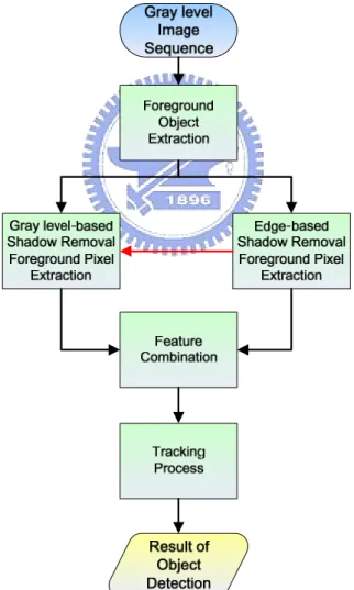
In this chapter, we will describe our algorithm in detail. Our Algorithm is composed of five blocks: Foreground Object Extraction, Edge-based Shadow

Removal Foreground Pixel Extraction, Gray level-based Shadow Removal Foreground Pixel Extraction, Feature Combination and Tracking Process. The

architecture diagram of our algorithm is shown in Fig. 3-1.

(21)

3.1. Moving Object Extraction

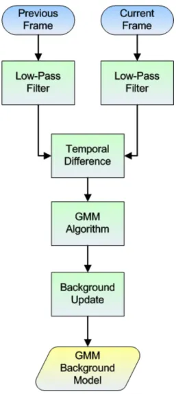
Figure 3-2 is the flow chart of foreground object extraction. The input of this block is gray level image sequence, and the output is the moving object with its minimum bounding rectangle. There are two common methods for obtaining foreground image. One is temporal difference, and another one is background subtraction. Temporal difference method is that we subtract frame t-1 from frame t, and the regions with obvious intensity variation are considered as foreground. Background subtraction is also in similar way but we use a constructed background image instead of frame t-1. Generally, the former one does a poor job of extracting all relevant feature pixels. Besides, by considering traffic monitoring system, cameras are usually set fixedly, so the background subtraction is a better choice for our proposed algorithm.

Fig. 3-2: Flow chart of foreground object extraction

Gaussian Mixture Model (GMM) is a common and robust method in background construction, so we also choose Gaussian Mixture Model (GMM) [14][15] to build background image. We will describe GMM in the following.

(22)

3.1.1. Gaussian Mixture Model for Background

Construction

Generally speaking, the intensity of each pixel varies in a small interval except the region of foreground objects. So, it is proper to use a Gaussian model to construct the background image. But in many surveillance videos, we would observe that there are waving leaves, sparking light, etc. In these situations, some background pixels would vary in several specific intervals. In other words, using 2, 3 or more Gaussian distributions to model a pixel will have better performance. We present the flow chart of GMM background construction in Fig. 3-3.

(23)

Firstly, we use a low-pass filter to reduce the noise. The GMM method models intensity of each pixel with K Gaussian distributions. The probability that a certain pixel has a value of X at time t can be written as. t

K , , , 1

(

t

)

k t

(

t

,

k t

,

k t

)

k

P X

ω

η

X

μ

=

∑

⋅

∑

_(3.1)

where K is the number of distributions that we used,

ω

k t, represents the weight of

k-th Gaussian in the mixture at time t,

μ

k t, is the mean of k-th Gaussian in the

mixture at time t, ∑ is the covariance matrix of the k-th Gaussian in the mixture at k t,

time t, and η is a Gaussian probability density function shown in Eq. (3.2)

( )

/ 2 _{1/ 2} 1 1 1 ( , , ) exp{ ( ) ( )} 2 2 | | T t t t _n t t t t t t X X X η π

μ

_{∑ =} ₋ ₋

μ

_∑ − ₋

μ

∑ (3.2)

where n is the dimension of data. In order to simplify the computation, it assumed that each channel of data is independent and have the same variance, and then can assume the covariance matrix as Eq. (3.3):

2

, I

k t σ_k

∑ = (3.3) We apply temporal difference to extract the possible background regions, and update pixels inside these regions. Then, we sort Gaussian distributions by the value of ω σ , and choose the first B distributions to be the background model, i.e. shown /

as Eq. (3.4): , 1 arg min( ) b k t b k B

ω

T = =

∑

> (3.4) When a new pixel is inputted (intensity is Xt+1), it will be checked against the K

distributions in turn. If the probability value is within 2.5 standard deviations, and this pixel is considered as background. Then, we update weight, mean, variance by Eq. (3.5), (3.6), (3.7):

(24)

, 1 (1 ) , ( , 1) k t k t Mk t ω + = −α

ω

+α + (3.5) 1 (1 ) 1 t ρ t ρXt

μ

+ = −

μ

+ + (3.6) 2 2 1 1 1 1 1 (1 ) ( ) ( ) T t t t t t t X X σ ₊ = −ρ σ +ρ + −μ + + −μ + (3.7) where α is a learning rate, Mk t, +1 is 1 for the model which matched and 0 for

remaining models, and Eq. (3.8) shows the second learning rate ρ.

1 , ,

(Xt | k t, k t)

ρ = αη + μ σ (3.8) Besides, the remaining Gaussians only update the weight. If there is no any distribution is matched, we replace the mean, variance and weight of the last distribution by Xt+1, a high variance and a low weight value, respectively. Figure

3-4 shows the constructed background image by GMM. Figure 3-5 shows the foreground image obtained by background subtraction.

(a) Video sequence (b) GMM Background Image Fig. 3-4: Background image construction by GMM

(a) Current image (b) Foreground image Fig. 3-5: Foreground image obtained by background subtraction

(25)

3.1.2. Morphological operation

After obtaining the foreground image, we are able to use the dilation and erosion operations to make the foreground more reliable. For example, we could use erosion to eliminate the small foreground which may be caused by noise, and use dilation to let the broken foreground objects could be more complete.

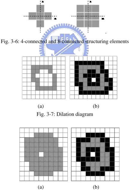
Dilation, in general, causes foreground objects to dilate or grow in size and erosion is corresponding to shrink. The amount and the way that they grow or shrink depend upon the choice of the structuring element. The two most common structuring elements (given a Cartesian grid) are the 4-connected and 8-connected sets. They are illustrated in Fig. 3-6.

.

Fig. 3-6: 4-connected and 8-connected structuring elements

(a) (b)

Fig. 3-7: Dilation diagram

(a) (b)

(26)

We can see the result of dilation operation in Fig. 3-7. The left side (Fig. 3-7(a)) is the original foreground object (marked as gray color). The result is the pixels mixed by the gray and black points as shown in Fig. 3-7(b). After dilation process, we can see the gray points are surrounded by black points and the foreground object becomes bigger. On the other hand, the result after erosion process is shown in Fig. 3-8. Figure 3-8(b) is the final result of erosion operation. The gray part in Fig. 3-8(b) is the result after process and the black part is eroded by operation.

3.1.3. Connected Component Labeling

Now, we need to segment the exact location and size of objects in the foreground image. The connected components labeling method is what we need for extracting the whole object from discrete points. Figure 3-9(a) shows that if without connected components labeling, all interesting points belong to 1 and others are 0. Although human can easily distinguish these two objects, but computer can’t tell the difference. Figure 3-9(b) shows that connected components labeling separate two un-overlap regions and paint them in different color where each color represents a single separated moving object.

(a) Before connected component (b) After connected component Fig. 3-9: Connected component labeling

(27)

In addition, we use a minimum bounding rectangle for each foreground object and record the coordinates of every bounding rectangle. And, we also record the label number of each foreground object for each bounding rectangle. The foreground object’s label number will help us to process the corresponding foreground pixels in the bounding rectangle. Some of the subsequent procedures that we will describe later only process inside the bounding region, and it assists us in reducing the computational loading. Figure 3-10 shows the minimum bounding rectangles that were marked as green.

Fig. 3-10: Moving Object with minimum bounding rectangle

3.2. Edge-based Shadow Removal Foreground

Pixel Extraction

In this section, we exploit the edge information of foreground object. The main concept of edge-based shadow removal foreground pixel extraction is that we keep the homogeneous property inside shadow region as much as possible and eliminate the boundary edge of object. Then, we can obtain the non-shadow edge feature. The flow chart, Fig. 3-11, is shown below.

(28)

Fig. 3-11: Flowchart of edge-based shadow removal foreground pixel extraction

3.2.1. Edge Extraction

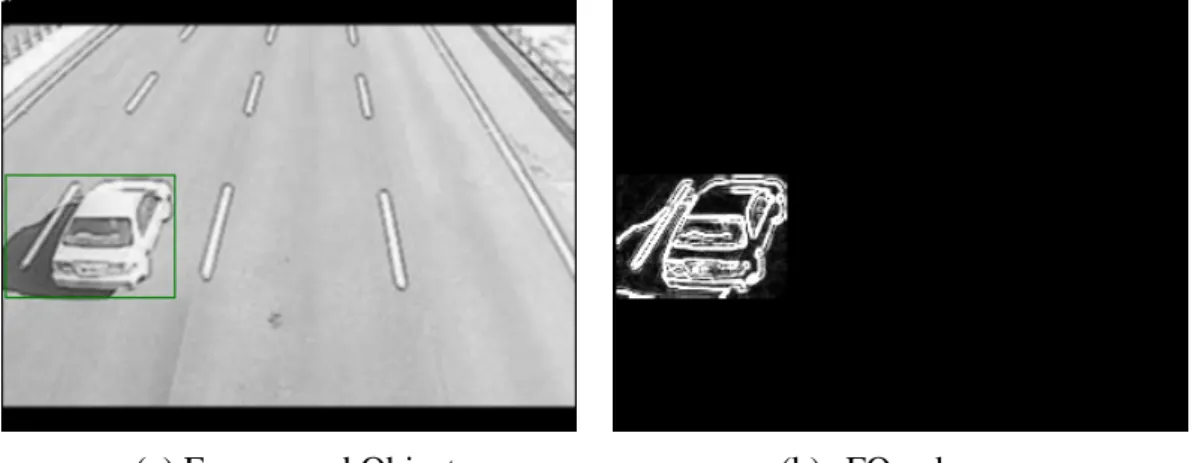
At first, we apply Sobel operation for both GMM background image and foreground object to extract the edge from them. We use the notation BI_edge to represent the edge extracted from background image and FO_edge_MBR to represent the edge extracted from foreground object. The subscript “MBR” means that we only process the operation inside the minimum bounding rectangle. Fig. 3-12 and Fig. 3-13 show the result of Sobel edge extraction from BI_edge and FO_edge_MBR , respectively.

(a) Background image (b) BI_edge Fig. 3-12: Sobel edge extraction from background image

(29)

(a) Foreground Object (b) FO_edge_MBR Fig. 3-13: Sobel edge extraction from moving object

In order to avoid extracting the undesired edge, for example, the edge of lane marking or the texture on the ground surface, we apply a pixel-by-pixel max operation from edge extracted background image and foreground object and notate it as

MBR

MI_edge which is shown as Eq. (3.9):

MBR MBR

MI_edge ( , )x y = max( FO_edge ( , ), BI_edge( , ) )x y x y , (3.9) where (x,y) represents the coordinate of the pixel, and an example of MI_edge_MBR is shown in Fig. 3-14.

(30)

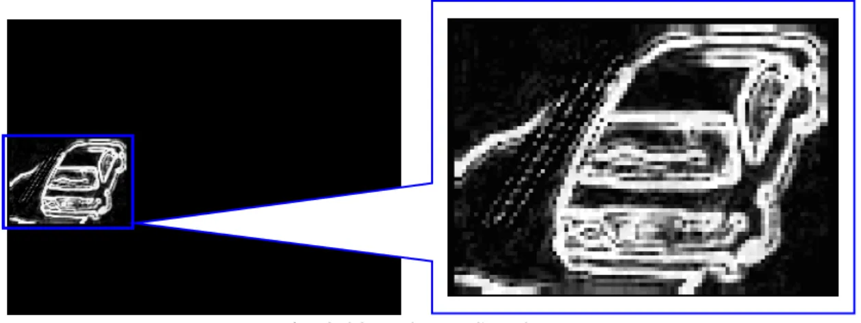
Then, we subtract BI_edge from MI_edge_MBR and obtain St_edge_MBR. Figure 3-15 shows the result of St_edge_MBR, and we can see the extracted edge of lane marking is reduced.

Fig. 3-15: The result of subtracting BI_edge from MI_edge_MBR

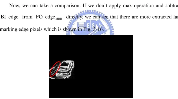
Now, we can take a comparison. If we don’t apply max operation and subtract BI_edge from FO_edge_MBR directly, we can see that there are more extracted lane marking edge pixels which is shown in Fig. 3-16.

Fig. 3-16: The result of subtracting BI_edge from FO_edge_MBR

Figure 3-17 shows that if the ground surface has texture, we also can see

MBR

St_edge is better than the result of subtracting BI_edge from FO_edge_MBR directly.

(31)

(a) Foreground Object (b) FO_edge_MBR

(c) Background Image (d) BI_edge

(e) St_edge_MBR (f) Subtract BI_edge from FO_edgeMBR

Fig. 3-17: Example of ground surface has texture.

From Fig. 3-16 and Fig. 3-17(f), we can see that the edge of lane marking or ground surface texture is presented (circled by red ellipse). By using max operation, we can reduce the effect that caused by lane marking or ground surface texture, and keep the homogeneous property that inside the shadow.

(32)

3.2.2. Adaptive Binarization method

After extracting edge, we use an adaptive binarization method to obtain binary image from St_edge_MBR. There are many binarization methods and can be classified into two categories generally. The first one is global binarization method like Otsu’s method [16]. Otsu tried to find a global threshold for whole image. Global method can provide a good result when the illumination over the image is uniform. But this assumption could not always be satisfied. Another one is local binarization method and this kind of method can provide a good result even in non-uniform luminance condition. Here, we apply Sauvola’s method [17][18]. Sauvola used a n x n mask that covers on image in each scanning iteration, by calculating mean and standard deviation of the pixel intensities in the mask, and then can determine a proper threshold. In order to suppress unimportant edge, we add a suppression term into the equation; Eq. (3.10) shows the revised equation.

final suppress ( , ) ( , ) ( , ) 1 s x y 1 t x y m x y k Th R ⎡ ⎛ ⎞⎤ = _⎢ + _⎜ − _⎟_⎥+ ⎝ ⎠ ⎣ ⎦ , (3.10) where ( , )m x y and ( , )s x y are the mean and standard deviation of mask that

centered at the pixel (x, y) respectively, R is the maximum value of the standard deviation (in gray level image, R=128), k is a parameter which takes positive values in the range [0.2, 0.5], and Th_suppress is a suppression term and its value is set as 50 empirically.

When t_final( , )x y is calculated, we use t_final( , )x y and take binarization at

location (x, y) according to Eq. (3.11),

MBR final MBR 0 St_edge ( , ) ( , ) BinI ( , ) 255

{

if x y t x y x y otherwise ≤ = , (3.11) where BinI_MBR is the result of binarization. In Fig. 3-18, we show the result of applying binarization method on St_edge_MBR.

(33)

(a) Binarization of Fig. 3-15 (b) Binarization of Fig. 3-17(e) Fig. 3-18: Examples of BinI_MBR

Here, we take a brief discussion of Th_suppress. If we don’t add this term into equation, we can see that the binarization points inside the shadow region were also extracted which was shown in Fig. 3-19.

Fig. 3-19: Obtained BinI_MBR without adding Th_suppress

We can enlarge St_edge_MBR and observe the shadow region. The region inside shadow still has very light texture (see Fig. 3-20), and by using original Sauvola’s method, the region with very light texture will also be extracted as binarization points. So, in order to keep the homogeneous property that inside the shadow region, the

suppress

(34)

Fig. 3-20: Enlarge St_edgeMBR

Instead of using a fixed threshold for binarization, the adaptive binarization method has another advantage. That is, we don’t have to manually set a proper threshold for each video scene, and it is a good characteristic for automatic monitoring system.

3.2.3. Boundary Elimination

Now, we have the binarized edge image BinI_MBR, and we are going to eliminate the outer border of BinI_MBR.

At first, we have to explain the motive of removing the outer border of BinI_MBR. By observing the foreground object, for example Fig. 3-21, we can find that:

¾ Shadow region and “real foreground object” have the same motion vector, and shadow is always adjacent to real foreground object.

¾ The interior region of shadow is edgeless (non-texture) and we call this kind of property as homogeneous. In other words, the edge that formed by shadow will appear at the outer border of foreground object. Oppositely, the interior region of real foreground object is non-homogeneous, and generally has much edge feature.

(35)

(a) Foreground object (b) BinI_MBR Fig. 3-21: Homogeneous property of shadow, example 1

Considering these two properties, the objective of removing shadow can be treated as eliminating the outer border and preserve the remaining edge which belongs to real foreground object.

But, the second property that we mentioned above may not always satisfied. Sometimes the interior region of shadow would have a little texture (lane marking etc.) like the example shown in Fig. 3-22. We can solve this kind of problem by the procedures that we have mentioned in section 3.2.1 and 3.2.2. We can see the

MBR

BinI of Fig. 3-22, although the interior region of shadow still has a little binarized edge points, but in the subsequent processing, we can easily cope with these noise-like points by just using a filter to filter them out.

(a) Moving object (b) BinI_MBR Fig. 3-22: Homogeneous property of shadow, example 2

(36)

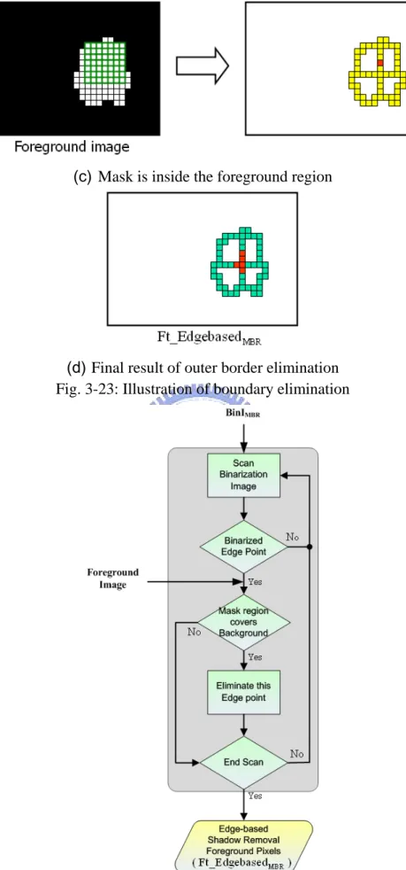
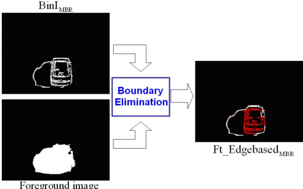
We use a 7 x 7 mask to achieve boundary elimination. As illustrating in Fig. 3-23, we put the green mask on the binarized edge points (marked as yellow color) of

MBR

BinI , and scan every point in the BinI_MBR sequentially. If the region which is covered by mask completely belongs to foreground image (marked as white point), we reserve this point (marked as red color); otherwise, we eliminate this point (marked as light blue point). After applying the outer border elimination, we can obtain the feature which is considered as non-shadow pixels, and notate it as

MBR

Ft_Edgebased . Figure 3-24 shows the flow chart of boundary elimination. In Fig. 3-25, we show an actual example, and the Ft_Edgebased_MBR is shown as red points.

(a) Using mask to scan BinIMBR

(37)

(c) Mask is inside the foreground region

(d) Final result of outer border elimination Fig. 3-23: Illustration of boundary elimination

(38)

Fig. 3-25: Example of boundary elimination

Before boundary elimination, there is an important pre-processing and we call it as broken foreground mending. In Fig. 3-26, we show a potential problem that may occur when apply boundary elimination. We can see Fig. 3-26(a); there are some holes in the foreground image and these holes are considered as background. So, after boundary elimination, we could see that, in Fig. 3-26(b), some of the binarized edge points inside the real foreground object are not reserved, and this kind of problem will harm the performance and stability of our proposed algorithm. Therefore, broken foreground mending is a critical pre-processing before boundary elimination.

(a) Foreground image (b) Ft_Edgebased_MBR Fig. 3-26: The problem caused by broken foreground image

(39)

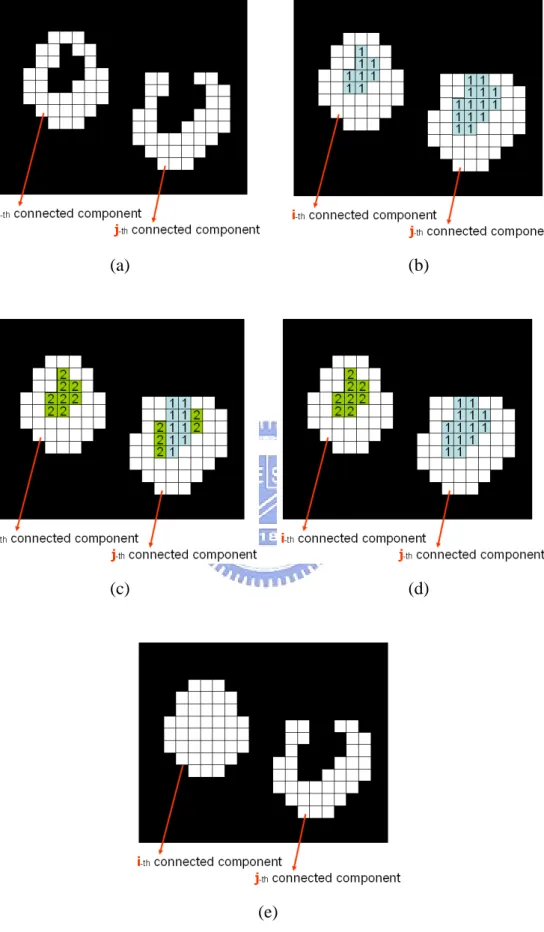
The broken foreground mending method is described as following steps:

Step 1:

We have a foreground image, for example, as Fig. 3-27(a). In this foreground image, there are two foreground objects. In the connected component labeling stage, we assign a label for each foreground object, and here, we denote as i and j. The i-th foreground object has a hole inside but the j-th foreground object doesn’t. Although j-th foreground object is not a broken foreground object, it has a concave shape.

We scan each row of the foreground object and label “1” to the non-foreground pixels (marked as black color) which fit the following condition:

z Non-foreground pixels are between two foreground pixels. In addition, these two foreground pixels must have the same connected component label.

After the horizontal scan, the result of this step is shown in Fig. 3-27(b).

Step 2:

Then, similarly, we scan each column of foreground object and increase value “1” to the non-foreground pixels which fit the same condition as mentioned above. Figure 3-27(c) shows the result in this step.

Step 3:

After the vertical scan, we will check that if any pixel which was labeled “2” is adjacent to pixel which was labeled “1”, then we modify the label of “2” to “1”. Figure 3-27(d) shows the result of checking.

Step 4:

Now, we are going to mend the broken foreground image. If the pixel is labeled as “2”, we modify this pixel from background pixel to foreground pixel, but if the pixel is labeled as “1”, we keep it as background pixel. Finally, we can obtain a mended foreground image which is shown in Fig. 3-27(e).

(40)

(a) (b)

(c) (d)

(e)

(41)

In Fig. 3-28, we show an actual example of broken foreground mending.

(a) Before mending process (b) After mending process Fig. 3-28: An example of broken foreground mending

3.3. Gray level-based Shadow Removal

Foreground Pixel Extraction

In this section, we are going to enhance and stabilize the shadow removing performance by utilizing a well-known “constant ratio” rule. We select some pixels which belong to shadow-potential region from foreground object and calculate darkening factor as training data, then build a Gaussian model for each gray level. Once the Gaussian model is trained, we can use the model to determine each of the pixels inside foreground object belong to shadow or not. Figure 3-29 shows the flow chart of gray level-based shadow removal foreground pixel extraction.

(42)

3.3.1. Constant ratio

Some authors had used the property of “constant ration” for shadow detection, [11] [19] [20] [21]. We use a notation I x y

(

,

)

to represent the intensity of a pixel which is on the coordinate ( , )x y of the current image and I x y

(

,

)

(

)

bg

,

)

sh bg , , I x y I x y = α (3.13)

3.3.2. Gaussian Darkening Factor Model Updating

(43)

data. In addition, the shadow-potential pixels selection procedure is automatic, namely, we don’t have to manually label pixels of shadow region from image frame.

Fig. 3-30: Each gray level has a Gaussian model.

The pixels which we select for Gaussian model updating must fit the following three conditions:

Pixels must belong to foreground object. Because shadow pixel must be contained by foreground image.

Intensity of a pixel (x, y) in the current frame is smaller than the intensity of the same pixel (x, y) in the background frame. Because shadow pixel must be darker than background’s.

The pixel is not a feature pixel which was obtained by edge-based shadow removal foreground pixel extraction. We use this constrain to reduce some pixels which probably belong to non-shadow pixel.

And in Fig. 3-31(b), the red pixels are the selected points and used for Gaussian model updating.

(44)

(a) Foreground object (b) Red points are the selected pixels Fig. 3-31: The selected pixels for Gaussian model updating

Once the pixels for updating were selected, now, we are going to update the mean and standard deviation of Gaussian model. Figure 3-32 is the flow chart of Gaussian darkening factor model updating. The darkening factor αk is calculated as Eq.

(3.14).

(

)

(

)

selected bg , , k k I x y I x y = α (3.14)

-th Gaussian model.

Fig. 3-32: Gaussian darkening factor model updating procedure

We set a threshold as a minimum number of updating times, namely, the updating times of each Gaussian model must exceed this threshold, and then, the model can be considered as stable. Besides, in order to reduce the computation loading of updating procedure, we limit that each Gaussian model could only be updated at most 200

(45)

3.3.3. Non-shadow Pixel Determination Task

Here, we are going to extract the non-shadow pixels by utilizing trained Gaussian darkening factor model. We sequentially scan the pixel in the foreground object from foreground image, and calculate the darkening factor, then, choose a trained Gaussian model for determination task. Figure 3-33 is the illustration of determination. We compute the difference between the mean of Gaussian model and the darkening factor, and check the difference is smaller than 3 times of standard deviation or not. If it is, the pixel is classified as shadow, otherwise, it is considered as non-shadow pixel and it is reserved as a feature pixel.

Fig. 3-33: Illustration of determination

Figure 3-34 is the flow chart of non-shadow pixel determination task, and we have a brief discussion of choosing trained Gaussian model. If the I_kbg

(

x y,

)

-th Gaussian model is not trained, we will select and check the nearby Gaussian models are marked as trained or not. In our program, we select the nearby 6 Gaussian models for checking, if there exists any trained Gaussian model, we choose the most nearest one.

(46)

Fig. 3-34: Flow chart of non-shadow pixel determination task

In Fig. 3-35(b), the pixels labeled by red color are the extracted feature pixels by this stage, and we denote the set of these pixels as Ft_DarkeningFactor_MBR.

(47)

(a) Foreground Object (b) Ft_DarkeningFactor_MBR

Fig. 3-35: An example of gray level-based non-shadow foreground pixel extraction

3.4. Feature Combination

After the processes that were mentioned in section 3.2 and 3.3, now, we have two obtained features. And we are going to integrate these two features and find the exact “real foreground object”. Figure 3-36 shows the flow chart of feature combination.

Fig. 3-36: Flow chart of feature combination

3.4.1. Integration by OR Operation

We integrate the two features by applying “OR” operation. Figure 3-37 is the illustration of OR operation, and Fig. 3-38 shows an example of OR operation and the obtained result is called feature integration image.

(48)

Fig. 3-37: Illustration of OR operation

(a) Foreground Object (b) Ft_Edgebased_MBR

(c) Ft_DarkeningFactorMBR (d) Feature integration image

Fig. 3-38: An example of integration

3.4.2. Labeling & Grouping and Size Filter

After we obtain the feature integration image, we are going to locate the real foreground object, namely, without including the shadow region. We apply connected component labeling and similarly use minimum bounding rectangle to indicate the real foreground object.

(49)

But before applying connected component labeling, we use a median filter to filter out some noise-like pixels. In Fig. 3-39(a), we can see that there are some pixels in the left part of feature integration image. These pixels are presented due to the influence by land marking (see Fig. 3-18(a)). In. Fig. 3-39(b), we can observe that after the median filter, these pixels are eliminated.

(a) Feature integration image (b) After filtering Fig. 3-39: Feature integration image filtering by median filter

By considering computational loading of median filter, we have a tip for decreasing it. The feature integration image is composed by red points and non-red points in the foreground image. So, we can just count which kind of point is more than another one, then we can know who the domination is.

Besides, after the median filtering, in order to make the left feature pixels to be more joined, we subsequently apply dilation operation. Figure 3-40 shows the result of dilation.

(50)

Now, we apply connected component labeling on dilated image. We also use minimum bounding rectangle for each independent region, and if any two minimum bounding rectangles are close to each other, then we will merge these two rectangles. We iteratively do checking and merging till there is no any rectangle can be merged together.

After labeling and grouping, Eq. (3.15) represents the size filter to eliminate the minimum bounding rectangle which its width and height are smaller than a threshold. The subscript “k” means the k-th minimum bounding rectangle.

min _MBR_Width MBR_ min _MBR_Height MBR_ { } { }

Eliminate -th Minimum Bounding Rectangle;

k k if Width Th AND Height Th k end < < (3.15)

Figure 3-41 shows some example of final located real object; the green rectangle represents foreground object and light blue rectangle means the final located real object.

Fig. 3-41: Examples of final located real object

3.5. Tracking Process

By aforementioned processing steps, we can extract the real foreground objects. But, occasionally, an “intact” real foreground object may have a fleeting split. For example, Fig. 3-42(a) and (b) show “intact” real foreground object which was extracted in frame 687 and 688, respectively. Figure 3-42(c) shows a split event in

(51)

(a) #687 (b) #688

(c) #689 (d) #690 Fig. 3-42: An example of split event

We can tackle this kind of problem by utilizing temporal information, i.e. the tracking process. Inputs of tracking process are the object list which we obtained from section 3.4 and the tracking table that obtained from last frame. The flow chart of tracking process is shown in Fig. 3-43.

(52)

3.5.1. Overlap region Analysis

With the object list and tracking table which was obtained from last frame, we can determine the matching state of each object in tracking table. Matching state represents the relation between the object in tracking table and the object in object list. Matching state can be classified into three categories: 1-to-1 matching, 1-to-many matching and many-to-1 matching; Fig. 3-44 is an illustration.

Fig. 3-44: Matching state illustration

Fig. 3-45: Overlap area of two objects

In Fig. 3-45, the red rectangle represents an object from tracking table, light blue one is an object from object list, and the green region is the overlap area between these two objects. We calculate the ratio of overlap area to the minimum area of two

(53)

overlap overlap / min( Obj_tracking table, Obj_object list)

Ratio = Area Area Area (3.16) And, a matching is established if the overlap ratio is large than a threshold.

If an object in tracking table only matches one object in object list, this situation is 1-to-1 matching. If an object in tracking table matches more than two objects in object list, we mark this object as 1-to-many matching. Oppositely, if there are more than two objects in tracking table match the same object in object list, these objects will be marked as many-to-1 matching.

3.5.2. Matching Process and Tracking Table Updating

After we have determined the matching state of each object in tracking table, now, we can do further process according to matching state and achieve the purpose of tracking. Figure 3-46 is the flow chart of matching process and tracking table updating.

(54)

Before the description of process for each matching state, we firstly interpret the lifetime of an object. If an object have put into the tracking table, we gave a lifetime “1” to this object. With each time of successful tracking of this object, we increase its lifetime by one.

¾ 1-to-1 Matching

This is the most simply situation. We update the information (width and height of minimum bounding rectangle, coordinate of central point, and motion vector) of corresponding object in tacking table directly.

¾ Many-to-1 Matching

We use Fig. 3-44 as an example to explain the process when matching state is many-to-1. In Fig. 3-44, there are 3 objects in tracking table correspond to the same object in object list. We check the life time of these 3 objects, if each of their lifetimes is larger than a threshold, ThOcclusion, then

the occlusion event is possibly occurred. Otherwise, these 3 objects may belong to same object.

When occlusion procedure is taken, we predict the respective position of objects in the next frame by using their motion vectors and update information of these 3 objects in tracking table. If replacement procedure is taken, we replace these 3 objects by the object in object list.

¾ 1-to-Many Matching

Similarly, we use Fig. 3-44 to interpret the process when matching state is marked as 1-to-many. There are two corresponding objects in object list. We check the distance of central point between these objects, and if the distance is large enough, then we split the object in tracking table and update information from these two objects. But if the distance is smaller than ThDist,

(55)

we merge them into one object and update the object in tracking table by new information.

¾ Non-matched Object in Object list

If there is an object which in object list is not matched by any object in tracking table, we consider this one may be an incoming object, and we add this one into tracking table.

In the next step, non-matching object reservation or elimination, we check the lifetime of every non-matching object in tracking table. If the lifetime is smaller than a threshold, we infer that this object may be a transient noise and remove this object from tracking table. If not, there are two possible situations. The first one is that failed object detection from image frame lead to no matching occurrence. The second one is that the object had left from image frame. For the first situation, we use object’s motion vector to predict the new coordinate in the next frame, but if the missing object is still not detected in the following two frames, then, we will delete this object from tracking table. For the second situation, it is reasonable to remove this object from tracking table. The basis of determining these two situations is by using the size of minimum bounding rectangle. If the width or height of minimum bounding rectangle is smaller than a threshold, we consider that the object is leaving from image frame.

Finally, we can determine the tracking result by examining lifetime of every object in tracking table. If the lifetime is larger than a threshold, the object can be established as extracted object.

(56)

Chapter 4 Experimental Results

In this chapter, we will show our results of shadow removal algorithm. We implemented our algorithm on the platform of PC with P4 3.0GHz and 1GB RAM. The software we used is Borland C++ Builder on Windows XP OS. All of the testing inputs are uncompressed AVI video files. The resolution of video frame is 320 x 240.

In section 4.1, we will show the experimental results of proposed algorithm on different scenes. Besides, a vehicle counting experiment is demonstrated in section 4.2. In section 4.3, we have a brief discussion of efficiency of our proposed algorithm.

4.1. Experimental Results of Shadow Removal

4.1.1. Experimental Results of Different Scenes

In the following, we show our experimental results under no occlusion situation in different scenes. At first, we use “green” rectangle to represent the result of foreground object detection without applying shadow removal, and “red” rectangle to represent the foreground object detection result with our proposed algorithm. In Fig. 4-1, we can see that the proposed algorithm can successfully detect real objects and remove the bad influence of shadow. Comparing with background, the intensity of shadow region is quite low and shadow region is very obvious. Besides, we also can observe that the shadow region is large. Figure 4-1(d), (f) show the results of big vehicle.

(57)

(a) (b) (c) (d) (e) (f)

Fig. 4-1: Experimental results of foreground object detection

In Fig. 4-2, we demonstrate the results under different shadow properties. Figure 4-2(a), shadow region is not large. Figure 4-2(c), the intensity difference of shadow and background is not quite much. In other words, the shadow region is “light”. Besides, its area of shadow is large. Figure 4-2(e), shadow region is “light” and its area is not large. No matter the shadow is obvious or non-obvious, and shadow’s area is large or small, the proposed method can have good results under these situations.

(58)

(a) (b) (c) (d) (e) (f)

In Fig. 4-3, we demonstrate the testing result of another scene. In addition, we also can detect the motorcycle and rider which is shown in Fig. 4-3(d).

(59)

(a) (b)

(c) (d)

Figure 4-4 shows the results of highway sequences which we obtained these testing videos from internet. We can see that the results of proposed algorithm are much better than left column.

(60)

(c) (d)

(e) (f)

4.1.2. Occlusion caused by shadow

Here, we demonstrate some examples of occlusion due to shadow influence. In Fig. 4-5 (a), (e), (g) and (i), we can see that two vehicles (or motorcycle and vehicle) were connected by shadow and (c) shows three vehicles were connected due to light shadow. Although shadow leads to occlusion, our method can deal with this kind of problem and the results are shown as (b), (d), (f), (h) and (j). Besides, in Fig. 4-5(i), we can see that three shadow regions were detected as one foreground object. With our method, we can have correct detection results.

(61)

(a) (b) (c) (d) (e) (f) (g) (h)

(62)

(i) (j) Fig. 4-5: Experimental results under occlusion situation

4.1.3. Discussions of Gray level-based Method

In section 3.3, we use darkening factor to enhance the performance and reliability of proposed algorithm. Here, we take a comparison of applying and not applying the method we mentioned in section 3.3.

Figure 4-6 shows a conspicuous example. Green rectangle represents the foreground object and red rectangle is detected object. The left column images, Fig. 4-6 (a)(c)(e), are the result of not applying gray level-based shadow removal foreground pixel extraction. In other words, the only feature can be used is “edge” feature which obtained from edge-based shadow removal foreground pixel extraction that we mentioned in section 3.2. But, if the object is edgeless (or textureless), the problem would appear. As the images shown in following left column, we can see that the roof of car is edgeless, so, the detected object will be broken or only the rear bumper can be detected. In the right column, Fig. 4-6 (b)(d)(f), if the gray level-based shadow removal foreground pixel extraction method is included, the edgeless problem can be solved.

(63)

(a) (b) (c) (d) (e) (f)

Fig. 4-6: Comparing the result of not applying and applying gray level-based shadow removal foreground pixel extraction

4.2. Vehicle Counting

We have 3 testing videos for vehicle counting. In Table 1, we list scene and shadow’s property of each video.

(64)

Table 1: Vehicle counting testing videos description Testing Video Scene Shadow Description Video FPS Video1 Highway Obvious and

Large 30 Video2 Highway Light and

Large 30 Video3 Expressway Obvious and

Large 25

Figure 4-7 shows the scene of each vehicle counting video. We partition Video1 into 6 partitions, Video2 into 13 partitions and Video3 into 2 partitions. Each of partition is about 2 minutes. There are 4 lanes in Video1 and Video2. In Video3, there are 2 lanes. In Table 2, we list the number of passing vehicles of each lane in every video. The number of passing vehicles is counted manually.

(a) Video1 (b) Video2 (c) Video3 Fig. 4-7: Scenes of vehicle counting videos

Table 2: Number of passing vehicles in each lane Testing Video Partition Number Lane1 (vehicles) Lane2 (vehicles) Lane3 (vehicles) Lane4 (vehicles) Video1 6 102 189 116 89 Video2 13 464 505 373 261 Video3 2 58 75 --- ---

(65)

We calculate accuracy rate for each partition by equation as Eq. (4.1): program manual manual | | 1 N N x 100% Accuracy rate N ⎡ ⎛ − ⎞⎤ = _⎢ −_⎜ _⎟_⎥ ⎝ ⎠ ⎣ ⎦ (4.1) where N_manual is the number of vehicles counted manually and N_program is the number of vehicles counted by program. Then, we will calculate the average accuracy rate for each video.

We use the foreground object detection result without shadow removal and the detection result of proposed algorithm as inputs in vehicle counting experiment. And, we will compare these two counting results. Table 3 shows the average accuracy rate of these three videos.

Table 3: Vehicle counting results Testing Video Comparing Method Lane1 (Average Accuracy rate) Lane2 (Average Accuracy rate) Lane3 (Average Accuracy rate) Lane4 (Average Accuracy rate) Video1 Without Shadow Removal 81.58 % 97.50 % 96.57 % 82.29 % With Proposed Algorithm 100 % 99.02 % 97.22 % 100 % Video2 Without Shadow Removal 92.88 % 96.27 % 95.55 % 89.51 % With Proposed Algorithm 97.59 % 99.31 % 99.68 % 99.26 % Video3 Without Shadow Removal 95.16 % 97.14 % --- --- With Proposed Algorithm 100 % 100 % --- ---

(66)

Table 4: Average accuracy of all lanes in each video

Testing Video Average Accuracy Rate

Video1 Without Shadow Removal 89.49 % With Proposed Algorithm 99.06 % Video2 Without Shadow Removal 93.55 % With Proposed Algorithm 98.96 % Video3 Without Shadow Removal 96.15 % With Proposed Algorithm 100 %

By observing the above results, we can see that the counting results of proposed algorithm are much better than the counting results without shadow removal. One of the reasons is that if an object’s shadow has not been eliminated, sometimes, this object will be determined on incorrect lane and lead to wrong counting.

Another reason is occlusion; two objects will be connected due to shadow, and be considered as only one object. Then, the wrong counting event will occur.

Now, we are going to discuss the errors that appear in our proposed algorithm. The first one is additional counting by mistakes. Figure 4-8 shows an example of additional counting by mistakes that occurs in testing videos. In Fig. 4-8, because the region of left red rectangle also has some texture, it is wrongly considered as an object.

(67)

Fig. 4-8: Additional counting by mistakes

Another error is that when two cars are occluded, it will be counted only one time and the wrong counting event happens. Figure 4-9 is an example of occlusion of two cars. And this kind of problem is not a focusing issue in this thesis.

Fig. 4-9: Occlusion of two cars

4.3. Execution Time Discussion

We use a video which has 4438 image frames, and cumulate the total processing time of executing proposed algorithm, and then calculate the processing average time of a frame. The processing average time is 13.84 milliseconds each frame. In other words, our algorithm can achieve 72.25 FPS and it is quite efficient.

快速的移動陰影移除演算法與其在交通流量偵測上的應用

國 立 交 通 大 學

電機與控制工程學系

碩 士 論 文

快速的移動陰影移除演算法

與其在交通流量偵測上的應用

An Efficient Moving Shadow Removal Algorithm

and Its Application of Traffic Flow Detection

研 究 生：吳晟輝

指導教授：林進燈 教授

快速的移動陰影移除演算法

與其在交通流量偵測上的應用

An Efficient Moving Shadow Removal Algorithm

and Its Application of Traffic Flow Detection

研 究 生：吳晟輝 Student：Cheng-Hui Wu

指導教授：林進燈 教授

Advisor：Dr. Chin-Teng Lin

國立交通大學

電機與控制工程學系

碩士論文

A Thesis

Submitted to Department of Electrical and Control Engineering

College of Engineering and Computer Science

National Chiao Tung University

in Partial Fulfillment of the Requirements

for the Degree of Master

in

Electrical and Control Engineering

March 2009

Hsinchu, Taiwan, Republic of China

快速的移動陰影移除演算法

與其在交通流量偵測上的應用

學生：吳晟輝

指導教授：林進燈 教授

國立交通大學電機與控制工程研究所

中文摘要

An Efficient Moving Shadow Removal Algorithm

and Its Application of Traffic Flow Detection

Student: Cheng-Hui Wu

Advisor: Prof. Chin-Teng Lin

Department of Electrical and Control Engineering

National Chiao Tung University

Abstract

致 謝

Contents

List of Tables

List of Figures

Chapter 1 Introduction

1.1. Motivation

1.2. Objective

1.3. Thesis organization

Chapter 2 Related Works

Chapter 3 Moving Shadow Removal

Algorithm

3.1. Moving Object Extraction

3.1.1.

Gaussian Mixture Model for Background

Construction

(

)

(

,

,

)

P X

ω

η

X

μ

=

∑

⋅

∑

ω

μ

( )

μ

μ

μ

ω

國立交通大學

碩士論文

研究生：吳晟輝

指導教授：林進燈教授

研究生：吳晟輝 Student：Cheng-Hui Wu

指導教授：林進燈教授

指導教授：林進燈教授

致謝