在無線網路中利用假設檢定達到偵測移動群組的機制

國

立

交

通

大

學

網路工程研究所

碩 士 論 文

在無線網路中利用假設檢定達到偵測移動群組的機制

Mobility Group Detection Using Hypothesis Testing in Wireless

Networks

研 究 生：張文馨

指導教授：陳 健 教授

在無線網路中利用假設檢定達到偵測移動群組的機制

Mobility Group Detection Using Hypothesis Testing in Wireless

Networks

研 究 生：張文馨 Student：Wen-Shin Chang

指導教授：陳 健 Advisor：Chien Chen

國 立 交 通 大 學

網 路 工 程 研 究 所

碩 士 論 文

A Thesis

Submitted to Institute of Network Engineering College of Computer Science

National Chiao Tung University In partial Fulfillment of the Requirements

For the Degree of Master

In

Computer Science and Engineering July 2009

Hsinchu, Taiwan, Republic of China 中華民國九十八年七月

在無線網路中利用假設檢定達到偵測移動群組的機制

研究生 : 張文馨 指導教授: 陳 健 國 立 交 通 大 學 網 路 工 程 研 究 所

中文摘要

本論文目的是在無線網路中，利用一群一起移動的行動裝置之間的距離、方 向及速度來偵測出他們是一個群組，並利用統計中的假設檢定來增加偵測的正確 率。隨著無線網路的快速發展，不論是利用基礎建設的WiMAX / 3G 系統，或是 無需基礎建設的MANET（Mobile Ad Hoc Network） / VANET（Vehicles Ad Hoc Network）都是目前相當重要的研究議題。在WiMAX / 3G 系統上，各個行動裝 置都需要與BS（Base Station）連線，再藉由BS連上網路。當行動裝置從一個地 方移動到另一個地方時，為了維持穩定的連線，必須發起換手的程序將連線換到 另一個訊號較好的BS。如果有一群行動裝置往相同的方向移動，例如在公車或 是捷運上的一群乘客，他們會在同時間個別發起換手的程序，則其換手過程中所 需耗費的控制訊息個數之總和是很大量的，這會造成換手延遲，甚至斷線。因此， 如果我們可以偵測出一群一起移動的行動裝置，而且將他們視為一個群組，則我 們就可以發起群組換手程序來取代個別換手程序，使handoff的負擔較低。在 MANET / VANET上，行動裝置無法獲得整體的資訊。行動裝置只能藉由他與鄰 居的相對位置及速度來偵測出哪一個鄰居是群組的成員。在MANET / VANET 上，群組的資訊可以使散佈資料更有效率。如果可以識別出群組中的某一點，則 我們可以將資料傳到群組中的一個點來取代將資料散佈到每一個點上。另外，行

動裝置要能長時間的運作，其電量管理是必要的，而群組的資訊可以用來幫助電 量管理。因為每一個行動裝置的電量都是由電池所提供，因此若是行動裝置可以 知道他自己的群組成員，則他可以選擇使用耗電量較小的Short range Interface來 溝通，而不需要一直使用耗電大的Long range Interface來溝通，這樣就能夠有效 的節省電量。因此，無論是在基礎建設的WiMAX / 3G系統或是無需基礎建設的 MANET / VANET下，群組偵測是很重要的研究。在本論文中，我們將探討如何 利用群組內行動裝置之間的關係去識別出一群一起移動的行動裝置，並利用這樣 的資訊將他們群組起來，這樣就可以改善網路的效能。在本論文中我們主要研究 可以分為:(1)在基礎建設式網路下，已知Leader資訊的情況，以Centralized的方式 偵測出群組，(2)在基礎建設式網路下，未知Leader資訊的情況，以Centralized的 方式偵測出群組，(3)在隨意式網路下，以Distributed的方式偵測出群組。以達到 在各種網路中，能夠有效率的分出群組的目的。最後利用模擬驗證所提出的方法。

Mobility Group Detection Using Hypothesis Testing in Wireless

Networks

Student: Wen-Shin Chang Advisor: Dr. Chien Chen

Institute of Network Engineering

National Chiao Tung University

Abstract

The purpose of this thesis is to identify a set of mobile devices which are moving as a group in wireless networks. We use the statistical hypothesis test to improve the correct detection rate. With the rapid development of wireless networks, the advance research in both infrastructure based WiMAX / 3G systems, and Mobile Ad Hoc Networks (MANET) / Vehicles Ad Hoc Networks (VANET) are very important. In the WiMAX / 3G systems, every mobile devices access to the networks by connecting with Base Stations (BS). In order to maintain the constantly connectivity to the networks, a moving mobile device must handoff from a BS to other BS with better coverage. However, if a group of mobile devices in the same direction, such as a group of passengers in the bus or a rapid train, they may initiates a handoff process individually at the same time. As a result, the number of handoff messages, which the BS needs to handle simultaneously are enormous. It may cause a handoff delay or even multiple calls drops. Therefore, if we can detect a group of mobile nodes in advance and treat them as a group instead of individual nodes, then we can initiate a group handoff to trim down total handoff overhead for a mobile group, In MANET / VANET, a mobile device is unable to obtain global information such as positions, direction and velocities of all nodes. A mobile device detects its group member only

by local information of its neighbored nodes. In MANET / VANET, group knowledge can help to spread information more efficiently. We can send a copy of information to one node of each group of mobile devices instead of spread information to every node if a group of nodes can be identified. Furthermore, group knowledge can help on energy management, which is an essential fact for the long duration operation of the MANETs. Since a mobile device of the MAVET is powered by the battery, if a node can know its group member, it can communicate with its group member using a short range interface instead of a more power hungry long range interface. In addition, we can use our method to implement cluster based algorithm for efficient routing and load balancing in MANET / VANET. Therefore, the group detection is an important research for both infrastructures based WiMAX / 3G systems, and MANET / VANET. In this thesis, we will explore the relationship between mobile devices to identify a group of nodes which travel as a group more accurately. We can make use of the group mobility to improve network performance. In this thesis, we focus on the following three topics: (1) Deign a centralize algorithm to detect a set of nodes which are traveling together in infrastructure based networks with a group lead. (2) Deign a centralize algorithm to detect a set of nodes which are traveling together in infrastructure based networks without a group lead. (3) Deign a distributed algorithm to detect a set of nodes which are traveling together in non-infrastructure based networks. Finally, simulation results show that our proposed approaches have a good group detection rate

誌謝

本篇論文的完成，我要感謝這兩年來給予我協助與勉勵的人。首先要感謝 我的指導教授 陳健博士，即使這段期間遭遇了不少的挫折，陳教授對我的指導 與教誨使我都能在遇到困難時另尋突破，在研究上處處碰壁時指引明路讓我得以 順利完成本篇論文，在此表達最誠摯的感謝。同時也感謝我的論文口試委員，簡 榮宏教授、沈建中教授，及清華大學的許健平教授，他們提出了許多的寶貴意見， 讓我受益良多。 感謝與我一同努力的學長陳盈羽、張哲維，由於我們不斷互相討論及在論 文上的協助，使我能突破瓶頸，研究也更為完善。另外我也要感謝實驗室的同學、 學弟們，蔡赫維、黃鼎鋒、孫冠宇、莊敬中等人，感謝他們陪我度過這兩年辛苦 的研究生活，在我需要協助時總是不吝伸出援手，陪我度過最煩躁與不順遂的日 子。 特別感謝我的朋友，及許多大學時代的好友們，他們在精神上給我莫大的 鼓勵，傾聽我內心 的聲音並帶給我無比的溫暖，指導我做出了許多正確的抉擇， 而不致迷失了自我。這些好朋友們就像是明燈般照亮了昏暗的旅程，並陪伴我度 過枯燥的研究生涯。 最後，我要感謝家人對我的關懷及支持，他們含辛茹苦的栽培，使我得以 無後顧之憂的專心於研究所課業與研究，我要向他們致上最高的感謝。

Table of Content

中文摘要 ... iii 

Abstract ... v 

誌謝... vii 

Table of Content ... viii 

Chapter 1: Introduction ... 1 

Chapter 2: Related work ... 6 

Chapter 3: Group Mobility Model ... 8 

3.1 Reference Point Group Mobility Model (RPGM) ... 8 

3.2 Reference Velocity Group Mobility Model (RVGM) ... 10 

Chapter 4: Calculate Confidence Index Method ... 12 

4.1 Calculate Confidence Index ... 12 

4.2 Hypothesis Testing ... 16 

Chapter 5: Mobility Group Detection ... 19 

5.1 Overview ... 19 

5.2 Centralized Mobility Group Detection with Leader ... 20 

5.3 Centralized Mobility Group Detection without Leader ... 21 

5.4 Distributed Mobility Group Detection ... 25 

Chapter 6: Simulation ... 27 

6.1 Simulation environment ... 27 

6.2 Metrics ... 29 

6.3 Simulation of Hypothesis Testing ... 30 

6.4 Simulation of Centralized Mobility Group Detection with Leader ... 33 

6.5 Simulation of Centralized Mobility Group Detection without Leader ... 36 

6.6 Distributed Mobility Group Detection ... 40 

Chapter 7: Conclusion ... 43 

List of Figure

Fig. 1、Infrastructure based networks ... 1

Fig. 2、MANET / VANET ... 2

Fig. 3、(a)The BS has the bus information;(b) The BS has no the bus information .... 3

Fig. 4、Reference Point Group Mobility Model ... 9

Fig. 8、Rejection Region and Accept Region ... 17

Fig. 9、The method of research and the purpose ... 19

Fig. 10、Centralized Mobility Group Detection in infrastructure based networks with a group lead... 21

Fig. 11、Centralized Mobility Group Detection in infrastructure based networks without a group lead ... 23

Fig. 12、Merge Algorithm ... 24

Fig. 13、Distributed Mobility Group Detection in non-infrastructure based networks ... 26

Fig. 14、The detect rate with different threshold in first environment. ... 31

Fig. 15、The error rate with different threshold in first environment. ... 31

Fig. 16、The detect rate with different threshold in second environment. ... 32

Fig. 17、The error rate with different threshold in second environment. ... 32

Fig. 18、The detect rate of centralized mobility group detection with leader in first environment. ... 33

Fig. 19、The error rate of centralized mobility group detection with leader in first environment. ... 34

Fig. 20、The detect rate of centralized mobility group detection with leader in second environment. ... 34

Fig. 21、The error rate of centralized mobility group detection with leader in second environment. ... 35

Fig. 22、The error rate of centralized mobility group detection without leader in first environment. ... 37

Fig. 23、The number of groups of centralized mobility group detection without leader in first environment. ... 37

Fig. 24、The error rate of centralized mobility group detection without leader in second environment. ... 38

Fig. 25、The number of groups of centralized mobility group detection without leader in second environment. ... 39

Fig. 26、The detect rate of distributed mobility group detection in first environment. ... 41 Fig. 27、The error rate of distributed mobility group detection in first environment. 41

Fig. 28、The detect rate of distributed mobility group detection in second environment. ... 42 Fig. 29、The error rate of distributed mobility group detection in second environment.

List of Equation

di,j(t) = Li(t) - Lj(t) ( 1) ... 12

ai,j(t) = min{ ai(t)-aj(t), 2π-(ai(t)-aj(t)) } ( 2) ... 13

mdi,j(t) = | mdi(t) - mdj(t)| ( 3) ... 13





 

t a

 

t or md

 

t T threshold d k c T k if T k T c T k T if c T k if j i j i j i              , , 0 * 2 / * 2 * 2 1 , , , ( 4) ... 13    

 

 

 

9 / , , 1 , , , / threahold z threshold T t md or t a t d k e c T k if c T k if j i j i j i z t k            ( 5) ... 14 ci,j(t)=(α*c1+β*c2+(1-α-β)*c3) ( 6) ... 21

detecti,j(t)=γ*ci,j(t)+(1-γ)* detecti,j(t-1) ( 7) ... 21

M(t)= γ*(mi,j(t))N×N+(1-γ)*(mi,j(t-1)) N×N ( 8) ... 22

detecti,j(t)=γ*ci,j(t)+(1-γ)*mi,j(t-1) ( 9) ... 22

 









 

 

_

 

             J I group j group i t t t J I j i m J I M J I J I M c c c t detect , , * , * 1 * ) 1 ( * * * 1 1 1 3 2 1 ,













( 10) ... 24 real correct

N

N

DetectRate



_{( 11) ... 29} real error

N

N

ErrorRate



_{( 12) ... 29}

Chapter 1: Introduction

The main purpose of this thesis is explore how to effectively detect a set of mobile devices which are moving as a group in both infrastructure based WiMAX / 3G systems, and Mobile Ad Hoc Networks (MANET) / Vehicles Ad Hoc Networks (VANET).

Due to the recent rapid development of wireless networks, there are more and more people using wireless mobile services through mobile devices nowadays. Today, wireless networks are classified into 2 categories, the infrastructure based networks, shown in Fig.1, and non-infrastructure based networks, shown in Fig.2. In Fig. 1, we show an infrastructure based wireless networks consists of a number of mobile devices that connect to the internet through the access to the fixed wireless based stations (BSs), such as WiMAX and3G. The non-infrastructure based networks consist of a number of mobile devices that connect with each other in the absence of fixed BS, such as MANET and VANET.

Fig. 2、MANET / VANET

In infrastructure based WiMAX / 3G systems, a group of mobile devices move, the active connections established between those mobile devices and the present BS may need to be transferred or handoff to other BS. If the handoff request is initialed by each mobile device, the numbers of handoff messages that the BS need to handle are enormous. It may cause a handoff delay or even multiple calls drops due to limited messages processing capability of the BS. For example, the passengers in the same bus or train are traveling in the same direction. If some of them use the mobile devices, they will handoff to the same BS almost at the same time. Thus the BS has to process a large number of handoff messages simultaneously. It may cause a handoff delay or even a call drop, if the BS is overloaded with the excessive number of handoff messages. In order to reduce the number of handoff messages, we can treat a set of mobile nodes as a group instead of individual nodes, then handoff through the a group handoff method.

In addition, in the non-infrastructure based MANET / VANET, the knowledge of a set of mobile devices which travel together in a period of time such as a car fleet can help to distribute the information more efficiently. In order to ensure the information can be spread out in MANET, the information must be distributed to each mobile

device. Therefore, it will waste a lot of resources, and one mobile device may receive duplicate information. However if a group of mobile devices can be identified, we can send a copy of information only to one mobile device instead of a group of mobile devices. Today, most of devices have more than two network interfaces, for example, WiMAX / Wihi or WiMAX / Zigbee. If a mobile device can know its group member, it can communicate with its group member using short range interface instead of more power hunger long range interface. In addition, we can use the group knowledge to implement a better cluster based routing algorithm for efficient resource utilization in MANET / VANET. A cluster based routing relies on the connectivity of the cluster heads (CH). With group knowledge we can have a better choice of cluster heads and maintain more stability of the clusters.

The purpose of this study is to explore how to detect a set of mobile device by their characteristic of movement and appropriate threshold. For example, in the bus, we regard a set of mobile device carried by the passengers as the same group. Therefore, we can improve handoff overhead by performing group handoff seamless. In addition, in MANET/VANET we can distribute data more efficiently with group knowledge. For example, we can spread the information to a specific MN instead of all MNs..

In the WiMAX / 3G systems, we make use of mobility information of mobile devices such as position, speed and moving direction to detect a group of mobile devices which are travel together. The issues of group detection in infrastructure-based wireless network can be classified into two categories: with group leader and without group leader. As shown as Fig.3(a), the bus has a mobile device which can be identified by the BSs as a group leader. Opposite, as shown as Fig.3(b), the bus carry no mobile device, thus the BSs have no information of the group leaders. Suppose that the BS has the information of the group leaders, the BS can detect a group by using the group leader’s mobility information as benchmarks to match up with the mobility information of other mobile devices. However, if the BS has no information of the group leaders; there are no benchmarks for comparison. Therefore, the mobility information of all mobile devices must be compared with each other which will increase the complexity of detection.

In the MANET / VANET, mobile device is unable to obtain global information such as positions, direction and velocities of all nodes. A mobile device detects its group members only by local information of its neighbored nodes.

According to the above descriptions, this thesis will explore how to detect a group of mobile devices by their mobility pattern in the infrastructure based networks and non-infrastructure networks. We employ statistical hypothesis test to obtain the suitable thresholds for an effective detection. In this thesis, we forces on the following three topics: (1) Deign a centralize algorithm to detect a set of nodes which is traveling together in infrastructure based networks with a group lead. (2) Deign a centralize algorithm to detect a set of nodes which is traveling together in infrastructure based networks without a group lead. (3) Deign a distributed algorithm to detect a set of nodes which is traveling together in non-infrastructure based

networks. First, we collect the positions of mobile nodes by signal strength. Then, we measure the difference of distance, moving angle and moving distance between two nodes. Calculate three confidence indexes by above measurements and appropriate thresholds. These thresholds are important. In order to improve the accuracy of the confidence index, we use the statistical hypothesis test to find the appropriate threshold. Finally, a probability of the same group between two nodes is obtained by confidence indexes and history data.

The remainder of the thesis is organized as follows. In chapter 2, we introduce some related works. In chapter 3, we present the existing group mobility models. In chapter 4, we describe how to calculate the confidence indexes and how to use the hypothesis testing to obtain the appropriate threshold. In chapter 5, we propose the mobility group detection. In chapter 6, we show the results of simulation experiments. Finally, in chapter 7, we summarize this paper.

Chapter 2: Related work

In terms of researching group mobility in wireless networks, we can divide it into four cases. The first one is to do the group mobility model. The second one is to detect the group. The third one is to predict the group. The fourth one is the clustering. We will discuss these four cases in the following.

The Group Mobility Model uses the group characteristics to simulate the relationship between nodes. So this model can simulate the group mobility. Therefore, it can further simulate the impact of specific network application or protocol. [1] introduce the Reference Point Group Mobility (RPGM) Model. In this model, each group has a reference center to be standard. [3] introduce the Reference Velocity Group Mobility (RVGM) model. This model is extending from the RPGM model. The difference between two models is that the RPGM model use reference point to be standard and the RVGM model use reference velocity to be standard. [10][11][12] also propose the different group mobility model.

The clustering is grouping the mobile nodes or fixed nodes. The most of clustering is grouping nodes by density, position or velocity. Therefore, it can not identify a set of nodes which is traveling together. It only know that the nodes together at some time. [6] propose a distributed clustering algorithm to grouping the mobile nodes by the mobile characteristic. [2][8] propose the clustering algorithm to improve the efficiency of hybrid routing and spread duplicate data. [14][15] also propose the different clustering for some specific application more efficiently.

The detection and prediction is to let the some application more efficiently. For example, routing, handover…etc. [5] propose the distributed detection algorithm. This algorithm different with our algorithm is that this algorithm is detect the group according to the connection time. [3][9] propose the prediction algorithm. These

algorithms use the mobile characteristics of group to predict the partition time. These algorithms make the routing more efficiently and completion rate of transfer data higher.

Chapter 3: Group Mobility Model

In this thesis, the group mobility model is very important. Some researchers have proposed group mobility models [1] [3]. The mobile node of group mobility model are moved by different features, and based on group-based movement. We can use this model to simulate. There are two kind of group mobility model. The reference point group mobility model (RPGM) is based on reference point. The reference velocity group mobility model (RVGM) is based on reference velocity. We will introduce advantages and disadvantages of the two types of group mobility model in the following.

3.1 Reference Point Group Mobility Model (RPGM)

The Reference Point Group Mobility model was developed by Hong et al. in [1]. In this model, mobile nodes are organized into group according to the logical reference center of group. The logical reference center determines the group's motion behavior, including position, direction, velocity…etc. Every member of group is uniformly distributed in the neighborhood of the logical reference center. Every node has the position of logical reference center and random motion vector. The random motion vector is derived by randomly deviating from the group leader. Therefore, its can present the movement of real behavior.

In the RPGM model, the group membership of a mobile node is represented by its displacement from the group reference center. For example, at time t, the location of node i in the group j is described as follows

Node location：X_j,i

 

t Y_j

 

t Z_j,i

 

t

Local displacement：Z_j,i

 

t is the random motion vector.

The example is the movement of group in Fig. 4. Every node has a group motion vectorV_gi . In time τ to τ+1, node moves to RP



 1



from RP

 

 according to the group motion vector GM V_gi and random motion vectorRM . Its will generate the new position of mobile node.

Fig. 4、Reference Point Group Mobility Model

The topologies can be generated with group-based node mobility in RPGM model. For partition prediction or mobility prediction, the RPGM model has a disadvantage. Only having instantaneous information of nodes position is difficult to predict the trend of changes in topology of the mobility group. Hence, when the group partition occurs, its can not have effective prediction, and the communication may be broke down.

the information is the position of mobile node. So, this disadvantage will not affect our research. Therefore, our simulation model is the RPGM model.

3.2 Reference Velocity Group Mobility Model (RVGM)

The Reference Velocity Group Mobility model was developed by Wang et al. in [3]. The RVGM model represents the mobile model as its velocityV 



V_x,V_y



, where

x

V and V are the velocity component in x and y directions. The RVGM model _y extends the RPGM model by proposing a velocity to present the mobility group and the mobility nodes. In this model, each group has a group velocity, and mobile nodes are organized into groups according to their logical reference velocity of group. Each mobile node has a group velocity and a random motion vector. The random motion vector is the local velocity deviation which can present the movement of real behavior.

In the RPGM model, the group membership of a mobile node is represented by the group velocity. For example, at time t, the velocity of node i in the group j is described as follows

Node velocity：V_j,i W_j

 

t U_j,i

 

t

Where Group velocity：W_j

 

t and Local velocity deviation：U_j,i

 

t are random variables.

The RVGM model has an advantage. The information of this model is velocity, so we can obtain the mobility of node immediately, and don’t need use the position to calculate the velocity. In Fig. 5, there are three difference groups. In a), it express the group distribution using the position of node. Every groups overlap, and the mobile nodes are scattered with no clear grouping. In b), the mobile nodes are concentrated

around the mean group velocity in their respective mobility groups, and the mobility groups are clear apparent.

The group can be separate immediately according to the velocity, but has a disadvantage. If there is a node which velocity is same as the group’s velocity, then this node belongs to this group, but this node so far away from the group. Therefore, we also need the node’s position.

Chapter 4: Calculate Confidence Index Method

This thesis proposed three methods to detect a set of mobile groups in wireless networks. Both of these methods need to derive a probability of the same group between two nodes. The same group probability can be obtained by three confidence indexes and some history data. In this chapter, we introduce how to calculate confidence indexes. In order to improve the accuracy of the detection probability, we use the statistical hypothesis test to find the appropriate thresholds. The detail description of our method is as following.

4.1 Calculate Confidence Index

We define three confidence indexes as indicates of the same group probability between any two nodes. The first confidence index c1 is based on the distance between two nodes. The second confidence index c2 is based on the difference of traveling direction between two nodes. And the third confidence index c3 is based on the difference of moving velocity between two nodes.

The equation for the differences of distance between Node i and Node j is given as follows:

di,j(t) = Li(t) - Lj(t) ( 1) Where di,j(t) is the distance between node i and node j at time t, and

Li(t)=(Xi(t),Yi(t)) and Lj(t)=(Xj(t),Yj(t)) are the positions of node i and node j at time t respectively.

The equation for the difference of traveling direction between two nodes is given as follows:

ai,j(t) = min{ ai(t)-aj(t), 2π-(ai(t)-aj(t)) } ( 2) Where ai,j(t) is the difference of the moving angle between node i and node j, and

ai(t) and aj(t) are the moving angles of node i and node j between time t-1 to t. The equation for the difference of moving distance between node i and node j is given as follows:

mdi,j(t) = | mdi(t) - mdj(t)| ( 3) Where mdi(t)=((Xi(t)-Xi(t-1))2+(Yi(t)-Yi(t-1))2)1/2 and mdj(t)=((Xj(t)-Xj(t-1))2+ (Yj(t)-Yj(t-1))2)1/2 is a moving distances of node i and node j during time t-1 to t. correspondingly.

For each parameter, we define a linear equation for the confidence index between node i and node j as following:





 

t a

 

t or md

 

t T threshold d k c T k if T k T c T k T if c T k if j i j i j i              , , 0 * 2 / * 2 * 2 1 , , , ( 4)

We use the following Fig. 6 to explain the linear equation. If the difference (k) smaller than threshold (T), then the confidence index (c) is 1. If k between T and 2*T, then the c is linear decrease to zero. If k bigger than 2*T, then the c is zero.

Fig. 6、The value of confidence index use linear equation

Where the exponential equation for the confidence index between node i and node j is as follows:    

 

 

 

9 / , , 1 , , , / threahold z threshold T t md or t a t d k e c T k if c T k if j i j i j i z t k            ( 5)

We use the following Fig. 7 to explain the exponential equation. If the difference (k) smaller than threshold (T), then the confidence index (c) is 1. If k bigger than T, then the c is exponential decrease to zero.

Fig. 7、The value of confidence index use linear equation

If the mobile node belongs to the group, then this node will move with this group and the difference of distance, direction and velocity between node and leader will smaller than Threshold. If the differences are bigger than threshold, it means the probability of same group is small. We use two kind of equation to calculate the confidence index. The exponential equation is more rigorous than linear equation. We will observe the differences that use the linear equation or exponential equation in chapter 6.

Therefore, we can obtain three difference values (k) by above Equation 1, 2, 3, and use the Equation 4 or Equation 5 to calculate three confidence indexes c1, c2, c3.

Then, the detect value can be calculate and to determine whether two nodes belong to the same group or not belong to the same group. Equation 4 is the linear equation. Equation 5 is the exponential equation. The mobile nodes have the specific difference

of distance, moving angle and moving distance with members. If the difference value which between two nodes bigger than threshold, two nodes maybe not belong to the same group. That is why we use the exponential equation. In the difference situation, the method of calculating the detect value is difference. These methods will show in chapter 5.

4.2 Hypothesis Testing

In order to obtain above three confidence indexes, we must have three thresholds. These thresholds are important to improve the accuracy of the detection rate. We use the statistical hypothesis test to find the appropriate thresholds. A statistical hypothesis test is a method of making statistical decisions using experimental data. The statistical hypothesis testing has been widely applied to different areas for establishing a set of statistical rules to reject or accept a hypothesis. The method of hypothesis testing involves a parameter θ whose value is unknown but must lie in a certain parameter space Ω. The certain parameter spaces Ω can be partitioned into two disjoint subsets Ω0 and Ω1. The unknown value of θ lies in Ω0 or in Ω1. The

hypothesis testing involves six steps which include: 1. Establish two assumptions, let Ho denote the null hypothesis that θ lies in Ω0 and Ha denote the alternative hypothesis

that θ lies in Ω1. 2. Set significance level α, it is a fixed probability that guaranteed

low probability of the hypothesis wrongly. 3. Choice a appropriate test statistic. 4. Decide the Rejection Region. 5. Take some sample to calculate the test statistic. 6. Conclude that our assumption is correct or not. Therefore, we can obtain the appropriate threshold. We give a example to explain the steps of the statistical hypothesis test as follows.

Step1: Establish the null hypothesis (Ho) and the alternative hypothesis (Ha). First, we assumption that there are more than 90% group members satisfy that the distances between members and leader are smaller than the threshold which is 81. Then, Ho：

0



  vs. Ha： ₀, where ₀ 90% and  is the value that we calculate. In this case, Ω0=[0,90] andΩ1=(90, 100].

Step2: Set significance level. Usually, the significance level α is chosen to be 0.01. The significance level as small as possible in order to guaranteed low probability of

the hypothesis wrongly

Step3: Choice a appropriate test statistic Z-test,

n X n X

Z _{ }0 _{ }0.9_{, where X is}

sample average,  is standard deviation, n is sample sizes.

Step4: Decide the Rejection Region. Ho： 90% vs. Ha： 90%, so this is the one-sided test. In fig.8, if _  Z_

n X

Z   0  _{, then reject Ho. Here, α=0.01 and}

504 . 0   Z .

Fig. 5、Rejection Region and Accept Region

Step5: Calculate the test statistic. Take 90 random samples. The x0.904 and

045038 . 0   , so 0.842558 90 045038 . 0 9 . 0 904 . 0 0 _  _   n X Z _ 

Step6: Conclude that is our assumption correct. We can reject Ho, because Z=0.842558 is bigger thanZ_ 0.504. Therefore, the threshold of the difference of

distance is 81.

We use the statistical hypothesis test to get the appropriate threshold, and then it will improve the accuracy of detection. Therefore, we can judge the groups accurately. If we don’t use the statistical hypothesis test to get the appropriate threshold, then the accuracy of mobility group detection will reduce. In chapter6, we will propose the simulation result to verify.

Chapter 5: Mobility Group Detection

This thesis uses two modes to detect the groups, because there are two kinds of networks. The communication of WiMAX / 3G systems is centralized, and the communication of MANET / VANET is distributed. Therefore, the problem is classified into 2 categories.

Fig. 6、The method of research and the purpose

5.1 Overview

In WiMAX / 3G systems, the BS collect the mobility information of mobile nodes, and use the trace information of each mobile node such as position, velocity and direction to detect the groups. There are two mobility group detection scenarios. First, Deign a centralize algorithm to detect a set of nodes which is traveling together in infrastructure based networks with a group lead. Second, Deign a centralize algorithm to detect a set of nodes which is traveling together in infrastructure based

networks without a group lead.

In MANET / VANET, every MN connects with each other in the absence of fixed BS. The MN can not obtain the trace information of all MNs. The MN only exchange local information such as relative position and relative velocity with its neighbor nodes. Therefore, a distributed mobility group detection method is proposed to detect a group of MNs.

5.2 Centralized Mobility Group Detection with Leader

In infrastructure based networks with a group lead, for example, in the bus, train or high-speed train, there are wireless device which as the leader of this group. In order to find the members of this group efficiently by the information of leader, we can collect the position of all nodes and leader in each time. We can calculate the velocity and moving direction by the position, and then to do comparison between leader and each of MNs. Therefore, we can detect a set of MNs which is traveling together in infrastructure based networks.

Algorithm 1 Mobility Group Detection Algorithm With Leader 1：Input：The position of all nodes P = [P1, …,Pn]

2：Output：A set of k groups G = [G1, …,Gk]

3：DETECT MOBILITY GROUP WITH LEADER 4：Choose one leader as reference node i

5：for i 1 to num_of_groups do 6： for j1 to num_of_nodes do

7： Obtain detecti,j(t) between node j and reference node i from

P as (1) - (4) and (6) - (7) or (1) - (3), (5) and (7) 8： if detecti,j(t) <δthen

9： node i and node j belong to the same group; 10： else

11： node j belong to the other group; 12： end if

14：end for

15：Obtain a set of k groups G = [G1, …,Gk]

16：END DETECT MOBILITY GROUP WITH LEADER

Fig. 7、Centralized Mobility Group Detection in infrastructure based networks with a group lead

Centralized Mobility Group Detection in infrastructure based networks with a group lead, show in Fig.10, first, the BS collect the information of all MNs, and then let leader as the reference node to compare with each of the other MNs. It can calculate the detect values. The BS starts to judge that which MN belong to this group. The detect value compare with the threshold δ. If the detect value bigger than the threshold, the MN belong to this group. If the detect value smaller than the threshold, the MN belong to the other group.

The equation for calculate the detect value is as follows, we use the confidence indexes that is introduce in chapter 4 and the history to calculate the detect vale.

ci,j(t)=(α*c1+β*c2+(1-α-β)*c3) ( 6)

detecti,j(t)=γ*ci,j(t)+(1-γ)* detecti,j(t-1) ( 7)

Where ci,j(t) is the confidence index between node i and node j at time t. c1, c2 and c3 are three confidence indexes as indicates of the same group probability between node i and node j. detecti,j(t) is the detect value which is the probability of the same group between node i and node j at time t.

5.3 Centralized Mobility Group Detection without Leader

In infrastructure based networks without a group lead, for example, in the concert or the parade, we can not obtain the information of leader. In order to find the

members of this group, we have to collect the position of all nodes in each time and calculate the velocity and the moving distance by the position. Then, we can detect a set of MNs which is traveling together in infrastructure based networks by the relationship between each MNs.

Centralized Mobility Group Detection in infrastructure based networks without a group lead, show in fig.11, first, the BS collect the information of all MNs, and then arbitrarily choose one node as the reference node to compare with the other randomly selected node j. If their detect value smaller than threshold δ, let node j be the reference node of other group. If their detect value bigger than threshold δ, they belong to the same group and let node j to join this group. Then, we continue to arbitrarily choose one node to compare with each of the other reference nodes and judge that this node belongs to which group. Until all nodes are to be selected, we have to do merge action. Finally, we can detect a number of set of nodes which is traveling together in infrastructure based networks.

In this case, the calculation of detect value is different from above case. The difference is history. We have to use a nn matrix to record the information between each MNs such as Equation8 where N is the number of MNs. Then, use Equation9 to calculate the detect value. If the detect value bigger than threshold δ,

they belong to the same group. If the detect value smaller than threshold δ, they do not belong to the same group.

M(t)= γ*(mi,j(t))N×N+(1-γ)*(mi,j(t-1)) N×N ( 8)

detecti,j(t)=γ*ci,j(t)+(1-γ)*mi,j(t-1) ( 9)

Where M(t) is a nn matrix to record the information between each MNs at time t. mi,j(t) is the probability of same group between node i and node j at time t. detecti,j(t) is the detect value which is the probability of the same group between node i and node j at time t. ci,j(t) is the confidence index between node i and node j at time t.

Algorithm 2 Mobility Group Detection Algorithm Without Leader 1：Input：The position of all nodes P = [P1, …,Pn]

2：Output：A set of k groups G’ = [G’1, …,G’k’]

3：DETECT MOBILITY GROUP WITHOUT LEADER

4：Arbitrarily choose one node as reference node i; 5：for j 1 to num_of_nodes do

6： repeat

7： Obtain detecti,j(t) between node j and Reference node i from P as (1) - (4), (6)and (9) or (1) – (3), (5), (6) and (9);

8： if detecti,j(t) <δthen

9： node i and node j belong to the same group; 10： else

11： node j belong to the other group; 12： end if

13： until all reference node already be choose

14： if node j is not group member of all reference node then 15： Let node j be a reference node;

16： end if 17：end for

18：Obtain a set of k groups G = [G1, …,Gk]; 19：MERGE( G , G’)

20：Obtain (mi,j(t))n×n from G’, if node i and node j belong to the same group then mi,j(t)= 1, else mi,j(t)=0;

21：Obtain M(t) from (mi,j(t))n×n and (mi,j(t-1))n×n as (8) 22：Obtain a set of k groups G’ = [G’1, …,G’k];

23：END DETECT MOBILITY GROUP WITHOUT LEADER

Fig. 8、Centralized Mobility Group Detection in infrastructure based networks without a group lead

Because we can’t prove that the reference node is in the center of group, a group may be divided in to small groups. Therefore, we have to do merge action. First, we have to calculate the center of each group. Then, let the center to be reference node and judge that which groups need to be merged. Show in fig.12.

The equation for calculate the detect value in merge action as follows:

 









 

 

_

 

             J I group j group i i j J I J I J I t m t M J I t M c c c t detect 1 1 * 1 * 1 * ) 1 ( * * * , , , 3 2 1 ,













( 10)

Where detectI,J(t) is the detect value which is the probability of the same group between group I and group J at time t. c1, c2 and c3 are three confidence indexes as indicates of the same group probability between group I and group J. Where MI,J(t-1) is history data record the information between group I and group J at time t-1. mi,j(t-1) is the probability of same group between node i and node j at time t-1.

Function 1 MERGE(G,G’)

1：Input：A set of k groups G = [G1, …,Gk] 2：Output：A set of k’ groups G’ = [G1, …,Gk’] 3：MERGE

4：for I1 to k do

5： Calculate the average of position of group I from G; 6：end for

7：Obtain P’ = [P’1, …,P’k]; 8：for I1 to k-1 do

9： for JI to k do

10： if Group J has not been merge then

11： Obtain detectI,J(t) between group J and group I from P’ as (1) – (4), (6) and (10) or (1) - (3), (5), (6) and (10);

12： if detectI,J(t) <δthen

13： Merge group I and group J; 14： end if

15： end if 16： end for 17：end for

18：Obtain a set of k’ groups G’ = [G1, …,Gk’]; 19：END MERGE

5.4 Distributed Mobility Group Detection

In non-infrastructure based networks, for example, in the car fleet, in order to find the members of this group efficiently, each node have to collect the position of all neighbors in each time and compare with each neighbors. Therefore, each node can detect that which node is belong to the same group, and then exchange the information with each neighbors. It will expand the scope of judgment to 2 hops. The distributed mobility group detection is show in fig.13. First, the mobile node collect the positions of all MNs, and then compare with each of the other MNs. It can calculate the detect values. The mobile nodes starts to judge that which MN belong to this group. The detect value compare with the threshold δ. If the detect value bigger than the threshold, the MN belong to this group. If the detect value smaller than the threshold, the MN belong to the other group. Because we just can obtain the one-hop information. Therefore, we have to exchange the information of local detection. First, we have to collect the information from one-hop member. Then, using the information of one-hop member to judge which MN is the two-hop member.

Algorithm 3 Distributed Mobility Group Detection Algorithm 1：Input：The position of neighbors P = [P1, …,Pn]

2：Output：A set M = [m1, …,mk]

3：DETECT MOBILITY GROUP WITH LEADER 4：Arbitrarily choose one neighbor j;

5：k  0;

6：for j  1 to num_of_neighbors do

7： Obtain detecti,j(t) between node i and neighbor j from P as (1) - (5) and (7) or (1) – (4), (6) and (7);

8： if detecti,j(t) < δ then

9： neighbor j and node i belong to the same group; 10： else

12： k  k+1; 13： end if

14： end for 15：end for

16：Obtain a set of group M’ = [m’1, …,m’k]; 17：Exchange information with members;

18：Obtain a Exchange Information Table EIT = [EIT1,…,EITh]; 19：for c  1 to h do

20： if (EIT→count)/ (k+1) > λ then

21： node (EIT→ID) and node i belong to the same group; 22： else

23： node (EIT→ID) and node i not belong to the same group 24： end if

25：end for

26：Obtain a set M = [m1, …,mk];

27：END DETECT MOBILITY GROUP WITH LEADER

Fig. 10、Distributed Mobility Group Detection in non-infrastructure based networks

In order to reduce the exchange information, the format of exchange information is (ID, group-member). Where the ID is the node id, the group-member is the group member id by the local detection. When node receives the exchange information, it will be collected into the Exchange Information Table(EIT). The format of Exchange Information Table is (ID, count). Where the ID is group member id in the exchange information, the count is the numbers of group member that detect this node belong to the same group.

Chapter 6: Simulation

In this thesis, we use the Reference Point Group Mobility model as our group mobility model. We write our group detection algorithms in the C language.. We use RPGM model to obtain the mobility information of each mobility device. With mobility trace of each mobile device we can detect a group of mobile devices which are traveling together using our algorithms. The simulations are performed in four parts. First simulation is to verify the importance of statistical hypothesis testing. We use some samples to obtain the appropriate thresholds by the statistical hypothesis testing. We compare detection rates with different thresholds and threshold obtained from the statistical hypothesis testing. Second, we perform the simulation for the Centralized Mobility Group Detection with Leaders. Third, we perform the simulation for the Centralized Mobility Group Detection without Leader. Fourth, we perform the simulation for the Distributed Mobility Group Detection. We will discuss the simulation environments, metrics, and results in the following subsections.

6.1 Simulation environment

We set up three simulation environments. In the first and second environments, all nodes are distributed in the 1000×1000m2 area. The first environment has 2 groups, and the number of nodes per group is 20. The second environment also has 2 groups, and the number of node per group is 20. Moreover, second environment adds another 300 individual nodes which move at random directions. The first environment has no noise and the second environment has noise. The detail parameters of the simulation are summarized in Table 1.

Table 1. The parameters of first and second simulation environments

Simulation time 900 s

Number of group 2

Number of node per group 20

Maximum speed 20 m/s Minimum speed 5 m/s Threshold1 (distance) 56 m Threshold2 (angle) 0.3 Threshold3 (velocity) 0.5 m/s δ 0.7 α 1/3 β 1/3

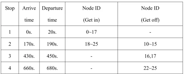
The third simulation environment is to imitate a bus route in the 3000×3000m2 area. This bus route has five bus stops and 26 mobile nodes which will get on and off the bus at the bus stops. The detail arrival and departure times of the bus and mobile nodes will get on and off at each stop are given in the following table.

Table 2. The bus simulation environment Stop Arrive time Departure time Node ID (Get in) Node ID (Get off) 1 0s. 20s. 0~17 - 2 170s. 190s. 18~25 10~15 3 430s. 450s. - 16,17 4 660s. 680s. - 22~25

5 880s. - - 0~9,18~21

Table 3、The parameters used in bus simulation Simulation time 900 s Number of node 26 Maximum speed 15 m/s Minimum speed 1 m/s Threshold1 (distance) 5 m Threshold2 (angle) 0.3 Threshold3 (velocity) 0.1 m/s δ 0.7 α 1/3 β 1/3

6.2 Metrics

We use the following two metrics to show the performance of our algorithm:

real correct

N

N

DetectRate



_{( 11)} Where N_correct is the number of nodes that are detected as a specific mobility group correctly while N_real is the number of nodes that belong to this group. The first metric reflects the proportion of the number of detection nodes to the number of real nodes. This value equal to 1 is the best.

real error

N

N

error

N is the number of nodes that are detected as this mobility group in error. The second metric reflects the proportion of the number of error detection nodes to the number of real nodes. This value equal to 0 is the best.

6.3 Simulation of Hypothesis Testing

The this simulation, we verify that the hypothesis testing is important. The value of γ are 0.1. We using the hypothesis testing to obtain the appropriate threshold is 1*threshold. Then we use 0.5*threshold, 1*threshold, 2*threshold and 4*threshold to calculate the confidence indexes. In following Fig. 14, 15, the equation for detect value is linear. In following Fig. 16, 17, the equation for detect value is exponential.

We first observed the detect rate. As show in Fig. 14, when the threshold is a half of the appropriate threshold, the best detect rate is 0.7 and the worst detect rate is 0.05. As show in Fig. 16, the detect rate of a half of the appropriate threshold is also bad. And the detect rate of the other thresholds is almost close to 1. It is because a half of the appropriate threshold is more rigorous than the other thresholds. Then we observed the error rate. As show in Fig. 15, 17, when the thresholds are bigger than the appropriate threshold, the error rate is higher. Therefore, if we can’t obtain the appropriate threshold, the detection will not be able to detect effectively.

Fig. 11、The detect rate with different threshold in first environment.

Fig. 13、The detect rate with different threshold in second environment.

6.4 Simulation of Centralized Mobility Group Detection

with Leader

First, we use the first and second environment to simulate the mobility group detection with leader. We comparing change of the detect rate and the error rate in different detect value calculation and γ. Where the value of γ are 0.1, 0.2 and 0.5. First we observed the detect rate in the first environment. In the following Fig. 18, when the equation is linear, the detect rate is 1. And when the equation is exponential, the detect rate is almost close to 1. It means that our method can detect all group members. Then we observed the error rate. As show in Fig. 19, the error rate is 0. It means that our method can clearly distinguish two groups when they mixed.

Fig. 15、The detect rate of centralized mobility group detection with leader in first environment.

Fig. 16、The error rate of centralized mobility group detection with leader in first environment.

We observed the detect rate and the error rate in the second environment. As show in Fig. 20, the detect rate is 1. In the following Fig. 21, the error rate is almost close to 0. It means that our method can clearly distinguish the group in the noise environment.

Fig. 17、The detect rate of centralized mobility group detection with leader in second environment.

Fig. 18、The error rate of centralized mobility group detection with leader in second environment.

Then, we use the third environment to simulate the mobility group detection with leader. The following table is the simulation result:

Table 4、The simulation result Time Mobile node ID belong to the same group 10~189 s. 0~17

190~449 s. 0~9, 16~25 450~679 s. 0~9, 18~25 680~900 s. 0~9, 18~21

The node 0 is the leader in this environment, so there is only one group. First, we collect the history data in time 0 to 9. At time 10, we start to detect the group. We use the linear equation and exponential equation to calculate the confidence indexes. The simulation results are the same. We observed the simulation result in the Table 4. Our

method can correct detect all of the mobile nodes which in the bus. It means that our method can clearly distinguish the group.

6.5 Simulation of Centralized Mobility Group Detection

without Leader

First, we use the first and second environment to simulate the mobility group detection without leader. In the case of no group lead, we comparing change of the error rate and the number of groups in different detect value calculation. Where the value of γ is 0.7. First we observed the error rate in the first environment. As show in Fig. 22, the error rate is 0. It means that we can distinguish the group when there is no leader’s information. Then we observed the number of groups in the first environment. As sow in Fig. 23, when the equation is linear, the number of groups is 2. When the equation is exponential, the average of number of groups is 3.02. It is bigger than the correct number. Because the exponential equation is more rigorous, the group may divided into a number of subgroups.

Fig. 19、The error rate of centralized mobility group detection without leader in first environment.

Fig. 20、The number of groups of centralized mobility group detection without leader in first environment.

We observed the error rate in the second environment. As show in Fig. 24, when the equation is linear, the error rate at beginning is 0.156 and reduced over time to 0.

When the equation is exponential, the error rate at beginning is 0.082 and reduced over time to 0. It is because we use the history to be reference. Then we observed the number of groups. As show in Fig. 25, the number of groups at beginning is smaller than 302 and increase over time to 302. It means that our method can clearly distinguish the group in the noise environment.

Fig. 21、The error rate of centralized mobility group detection without leader in second environment.

Fig. 22、The number of groups of centralized mobility group detection without leader in second environment.

We use the third environment to simulate the mobility group detection without leader. The following table is the simulation result:

Table 5、The simulation result

Time Mobile node ID belong to the same group 10~179 s. 0~17 18~25 180~189 s. 0~25 190~449s. 0~9, 16~25 10~15 450~679 s. 0~9, 18~25 10~15 16, 17 680~900 s. 0~9, 18~21 10~15

16, 17 22~25

First, we collect the history data in time 0 to 9. At time 10, we start to detect the group. We use the linear equation and exponential equation to calculate the confidence indexes. The simulation results are the same. There is no leader information in this environment, so we detect more than one group. We observed the simulation result in the Table 5. Our method can correct detect all of the mobile nodes which in the bus or moving together. It means that our method can clearly distinguish the group.

6.6 Distributed Mobility Group Detection

In the case of Distributed Mobility Group Detection, we comparing change of the detect rate and the error rate in different detect value calculation and γ. Where the value of γ are 0.1 and 0.5, the communication range is 100m. First we observed the detect rate in first environment. As show in Fig. 26, when the equation is linear, the detect rate is almost close to 1. When the equation is exponential, the average of detect rate is 0.861. It is because the exponential equation is more rigorous. Then we observed the error rate in first environment. As show in Fig. 27, the error rate is almost close to 0. When the equation is exponential and γ=0.5, the error rate at time=900 is 0.015 which is bigger than the other cases. It is because the value of γ is 0.5. The history information is much less.

Fig. 23、The detect rate of distributed mobility group detection in first environment.

Fig. 24、The error rate of distributed mobility group detection in first environment.

We observed the detect rate in second environment. As show in Fig.28, the average of detect rate by linear equation is big 0.124 than the average of detect rate by exponential equation. It is because the linear equation is much loose. Then we observed the error rate in second environment. As show in Fig.29, when the equation is linear, the average of error rate is 0.0014. When the equation is exponential andγ

=0.1, the average of error rate is 0.0006. When the equation is exponential andγ=0.5, the average of error rate is 0.0015. The error rate is lowest in exponential equation and γ=0.5. It is because that the exponential equation is rigorously.

Fig. 25、The detect rate of distributed mobility group detection in second environment.

Chapter 7: Conclusion

In the infrastructure based networks, the handoff procedure is closely related to the number of handoff message. If the number of handoff message is large, it may cause the handoff delay. In the non-infrastructure based networks, the efficiency of information dissemination is closely related to the routing. In order to improve the efficiency of handoff and information dissemination, it has to join the concept of group mobility.

This thesis proposed three methods that are to detect a set of nodes which is traveling together in the infrastructure based networks and non-infrastructure based networks. These three methods need the threshold to calculate the confidence index. Therefore, we use statistical hypothesis testing to get the appropriate threshold. In the infrastructure based networks, the problem can be classified into 2 classifications, the Centralized Mobility Group Detection with a group lead, the Centralized Mobility Group Detection without a group lead. The BS use difference method to detect the group in difference situation. In the non-infrastructure networks, MN can not obtain the global information. Therefore, each MN has to use the local information to detect the group member and exchange data to get more information. In our simulation, we can observe that use our method can achieve well detect rate and accuracy in wireless networks.

References:

[1] X. Hong, et al. , ”A Group Mobility Model for Ad Hoc Wireless Networks,” In Proceedings of the ACM International Workshop on Modeling and Simulation of Wireless and Mobile Systems, pp. 53-60, August 1999.

[2] JiunLong Huang, MingSyan Chen, WenChih Peng,” Exploring Group Mobility for Replica Data Allocation in a Mobile Environment,” In Proceedings of the ACM International Conference Information and Knowledge Management, pp. 161–168, 2003.

[3] K. H. Wang, B. L, “Group Mobility and Partition Prediction in Wireless Ad-Hoc Networks,” In Proceedings of IEEE International Conference on Communications, pp. 1017-1021, April 2002.

[4] B. Li.,”On Increasing Service Accessibility and Efficiency in Wireless Ad-Hoc Networks with Group Mobility,” Wireless Personal Communications, vol. 21, no. 1, pp. 105–123, April 2002.

[5] Peng Min, Lu Hancheng, Hong Peilin, Zhou Xiaobo, ”MODEL:A Framework for Mobility Detection with Local Information,” In Proceedings of the IEEE Vehicular Technology Conference, May 2008.

[6] Yan Zhang, Jim Mee Ng, “A Distributed Group Mobility Adaptive Clustering Algorithm for Mobile Ad Hoc Networks,” In Proceedings of IEEE International Conference on Communications, pp.189-202, May 2008.

[7] Wen-Tsuen Chen, Po-Yu Chen, ”Group Mobility Management in Wireless Ad Hoc Networks,” In Proceedings of the IEEE Vehicular Technology Conference, pp. 2202–2206, Fall 2003.

[8] A. B. McDonald and T. Zntai, “A Mobility Based Framework for Adaptive Clustering in Wireless Ad-Hoc Networks,” In IEEE Journal on Selected Areas in Communications, Vol. 17, No.8, pp. 1466-1487, 1999.

[9] W. Su, S.-J. Lee, and M. Gerla, “Mobility Prediction in Wireless Networks,” In Proceedings of IEEE Military Communications Conference, pp. 491-495, Oct. 2000.

[10] C. Tuduce and T. Gross, “A Mobility Model based on WLAN Traces and Its Validation,” In Proceedings of IEEE INFOCOM, vol. 1, pp. 664-674, March 2005.

[11] V. Vetriselvi and R. Parthasarathi, “Trace Based Mobility Model for Ad Hoc Networks,” In Proceedings of Third IEEE International Conference on Wireless and Mobile Computing, Networking and Communications, pp. 81-81, Oct. 2007. [12] J. M. Ng and Y. Zhang, "A Mobility Model with Group Partitioning for Wireless

Ad hoc Networks," In Proceedings of IEEE International Conference on Information Technology and Applications, pp.289-294, July 2005.

[13] L. Badia and N. Bui, “A group mobility model based on nodes’ attraction for next generation wireless networks,” In Proceedings of the International conference

on Mobile technology, applications & systems, Oct 2006.

[14] J. MacQueen, ”Some Methods for Classification and Analysis of Multivariate Observation,” In Proceedings of the Fifth Berkeley Symposium on Mathematical Statistic and Probability, vol. 1, pp. 281-297, 1967.

[15] Gianluigi Folino and Giandomenico Spezzano. “An adaptive flocking algorithm for spatial clustering,” In Proceedings of the Parallel problem solving from nature, pp. 924-933, 2002.

[16] T. Hara, ”Effective Replica Allocation in Ad Hoc networks for Improving Data Accessibility,” In Proceedings of IEEE INFOCOM, vol. 3, pp. 1568-1576, 2001. [17] H. DeGroot, J. Schervish, “Probability and Statistics,” Third Edition,