國
立
交
通
大
學
多媒體工程研究所
碩
士
論
文
基於視角的連續自我碰撞偵測以及在圖形處理
器上之加速
View-based Continuous Self-Collision Detection with
Graphics Hardware Acceleration
研 究 生:鄭游駿
指導教授:黃世強 教授
基於視角的連續自我碰撞偵測以及在圖形處理器上之加速
View-based Continuous Self-Collision Detection with Graphics Hardware
Acceleration
研 究 生 :鄭游駿
Student :Yu-Chun Cheng
指 導 教 授 :黃世強
Advisor :Sai-Keung Wong
國 立 交 通 大 學
多 媒 體 工 程 研 究 所
碩 士 論 文
A Thesis
Submitted to Institute of Multimedia Engineering College of Computer Science
National Chiao Tung University in partial Fulfillment of the Requirements
for the Degree of Master
in
Computer Science July 2011
Hsinchu, Taiwan, Republic of China
基於視角的連續自我碰撞偵測以及在圖形處理
器上之加速
研究生:鄭游駿
指導教授:黃世強 教授
國 立 交 通 大 學
多 媒 體 工 程 研 究 所
摘要
在這篇論文中,我們提出了一個新的基於視角的方法來對可變形物體進行連 續自我碰撞偵測,首先我們會利用一個點或是一條線段等簡單的幾何元件來當作 基準,這些基準元件會被放置於可變形物體的內部,在整個物理模擬過程中,我 們會確保它們不會穿過該可變形物體,接著,我們會利用這些基準元件來定義可 變形物體中所有三角形的方向,根據每一個三角形的方向將整個可變形物體的三 角形做分堆,放進不同的視角集合裡,這個過程稱為視角測試。如果所有的三角 形都朝向基準元件,則該可變形物體中是沒有自我碰撞存在的,否則,我們將會 對某些成對的視角集合做進一步地處理。視角測試的計算量遠小於傳統的方法, 使用我們的方法來偵測自我碰撞,整體的效能是比較快的。此外,由於我們的方 法適合於平行運算,所以我們進一步地利用圖形處理器來實作我們的方法,進而 加速及改進整體的效能,實驗的數據顯示,利用我們的方法來偵測可變形物體的 自我碰撞,其效能不管是在 CPU 上還是 GPU 上都是令人滿意的。View-based Continuous Self-Collision Detection
with Graphics Hardware Acceleration
Student: Yu-Chun Cheng
Advisor: Sei-Keung Wong
National Chiao Tung University
Institute of Multimedia Engineering
Abstract
In this thesis, we propose a novel view-based approach for continuous self-collision detection with deformable triangle meshes. At first, we compute a simple geometric prim-itive, such as a point or a line segment. The primitive is put inside the deformable object, and we assume that it does not penetrate the object during the simulation. Then, the prim-itive is employed to determine the orientation of all triangles of the object. The triangles are divided into several view sets according to their orientation each frame, and this proce-dure is called view test. If all triangles face the primitives, then the object is self-collision free. Otherwise, self-collision is detected for certain pairs of the view sets. The computa-tion of the view-based approach is lower than tradicomputa-tional methods, such as regular patches division and contour tests. Besides, our approach is suitable for parallel computing. We implement the view-based approach on GPUs with CUDA and improve the performance significantly. The experimental results show that the performance of the view-based ap-proach for continuous self-collision detection is satisfied on both CPUs and GPUs.
Acknowledgements
I would like to thank my advisor, Dr. Sai-Keung Wong, for his guidance, assistance, and inspirations. His suggestion is very helpful for me to obtain the idea and develop the framework of the thesis. In addition to support my work, he cared about our health and gave much useful advice of philosophy of life to us. I would also like to thank my thesis committee members, Dr. Ming-Te Chi and Dr. Wen-Chieh Lin, who evaluated my thesis. I would like to thank all the labmates for their comments and help. They are so kind and cute so that I can learn in a cheerful environment. Last but not the least, I thank my parents for their unconditional support and patient. I hope it's my turn to take care of them.
Yu-Chun Cheng July 2011
Contents
摘要 i
Abstract ii
Acknowledgements iii
Table of Contents iv
List of Figures vii
List of Tables x 1 Introduction 1 1.1 Motivation . . . 4 1.2 Overview . . . 4 1.3 Contribution . . . 6 1.4 Organization . . . 7 2 Related Work 8 3 View-based Scheme 11 3.1 View-based Models . . . 11
3.2 View Tests with a Point . . . 13
3.3 View Tests with a Line Segment . . . 17
3.5 View-Point Scheme . . . 29
3.6 View-Line Scheme . . . 32
3.7 Discussion . . . 34
3.7.1 View-based approach vs. traditional approach . . . 34
3.7.2 View-point vs. view-line . . . 35
4 Implementation on CPUs 37 4.1 Preprocessing . . . 37
4.1.1 Acceleration structure construction . . . 37
4.1.2 View primitives computation . . . 39
4.1.3 Feature assignments . . . 40
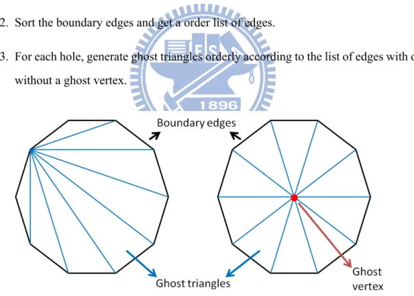
4.1.4 Ghost triangles generation . . . 40
4.2 View Tests . . . 42 4.2.1 View-point scheme . . . 42 4.2.2 View-line scheme . . . 42 4.2.3 Triangle clusters . . . 43 4.3 Boundary Handling . . . 44 4.4 Traversal . . . 44 4.5 Elementary Tests . . . 47 5 Implementation on GPUs 49 5.1 GPU Architecture . . . 49
5.2 Use of Data on GPUs . . . 52
5.2.1 Static data . . . 52
5.2.2 Dynamic data . . . 52
5.2.3 Global memory allocation in advance . . . 54
5.3 View Tests . . . 55
5.3.1 Vertex region determination . . . 56
5.3.2 Triangle type determination . . . 56
5.5 Traversal . . . 60
5.6 Elementary Tests . . . 68
6 Results and Discussion 70 6.1 Animation Benchmarks . . . 70
6.2 Results on CPUs . . . 77
6.3 Results on GPUs . . . 82
6.4 Differences of Each Step on CPUs and on GPUs . . . 84
6.5 Vertex Movement within a Frame . . . 88
6.6 Improvement with Triangle Clusters . . . 88
6.7 vBVHs Construction . . . 88
6.8 Discussion . . . 89
6.8.1 Closed and unclosed meshes . . . 89
6.8.2 Ghost triangles with or without ghost vertices . . . 90
6.8.3 Comparison between the view-point and view-line scheme . . . . 91
7 Conclusion and Future Work 94 7.1 Conclusion . . . 94
7.2 Future Work . . . 95
List of Figures
1.1 Two types of collision detection. Let ∆t be the time step. . . . 3
3.1 The view-based point model. . . 12
3.2 The view-based line segment model. . . 12
3.3 Triangle orientation determination with a view-point at a certain time. . . 13
3.4 Triangle orientation determination with a view-point over a time interval. 16 3.5 Triangle orientation determination with a view-line at a certain time. . . . 17
3.6 Triangle orientation determination with a view-line at a certain time when the triangle lies in multiple regions. . . 20
3.7 Triangle orientation determination with a view-line at a certain time when the triangle lies in multiple regions. . . 20
3.8 Triangle orientation determination with a view-line over a time interval when the triangle moves across multiple regions. . . 22
3.9 Triangle orientation determination with a view-line over a time interval when the triangle moves across multiple regions. . . 25
3.10 A 2D closed curve with a ray shot outward. . . 26
3.11 2D closed curves with self-intersection. . . 27
3.12 A 2D unclosed curve with self-intersection. . . 29
3.13 An example of handling unclosed objects. . . 29
3.14 Negatively oriented edges according to the view-point and view-line schemes. 36 4.1 Ghost triangles with and without a ghost vertex. . . 41
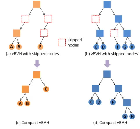
4.3 Marking process of vBVHs. . . 46
4.4 Skipped nodes in the vBVHs are adopted in order to compress the vBVHs. 47 5.1 Summary table of various GPU architecture. (The information is quoted from [NVI09].) . . . 51
5.2 Level-order node list of the BVH. . . 53
5.3 Preprocess the triangle type list before performing boundary handling. . . 59
5.4 The triangle type list. . . 63
5.5 Preprocess the triangle type list before performing traversal. . . 64
5.6 Examples for history lists. . . 66
5.7 History list with many redundant nodes and reasonable nodes. . . 66
5.8 PCPs array preprocessing. . . 69
6.1 A series of snapshots of Ani. one. The first row and the second row are viewed from different viewpoints. . . 72
6.2 A series of snapshots of Ani. two. The first row and the second row are viewed from different viewpoints. . . 72
6.3 A series of snapshots of Ani. three. . . 73
6.4 A series of snapshots of Ani. four. . . 73
6.5 A series of snapshots of Ani. five. . . 74
6.6 A series of snapshots of Ani. six. . . 74
6.7 The snapshots of Ani. one and two in wireframe. . . 75
6.8 The snapshots of Ani. three with ghost triangles. . . 75
6.9 The snapshots of Ani. five with ghost triangles. . . 76
6.10 The snapshots of Ani. six with ghost triangles. . . 76
6.11 The numbers of triangles of all kinds of view sets with the view-point scheme for the six benchmarks. . . 80
6.12 The numbers of triangles of all kinds of view sets with the view-line scheme for the six benchmarks. . . 81
6.13 Comparisons of the number of negatively oriented triangles without con-sidering violated triangles between the point scheme and the view-line scheme. . . 93 7.1 Boundary edges roll and lay down. . . 96
List of Tables
5.1 Salient features of device memory for devices of compute capability 1.x. The information is quoted from [NVI10a]. . . 50 6.1 Model complexities and information of ghost triangles for unclosed models. 71 6.2 Execution time (in ms) of each step with the view-point scheme on CPUs
for continuous self-collision detection. . . 79 6.3 Execution time (in ms) of each step with the view-line scheme on CPUs
for continuous self-collision detection. . . 79 6.4 Timing comparisons (in ms) between our view-based approach, AABB,
16-DOP, and ICCD for continuous self-collision detection. . . 79 6.5 Execution time (in ms) of performing traversal in the beginning to obtain
the initial history nodes. . . 82 6.6 Execution time (in ms) of each step with the view-point scheme on GPUs
for continuous self-collision detection. . . 82 6.7 Execution time (in ms) of each step with the view-line scheme on GPUs
for continuous self-collision detection. . . 83 6.8 Speed-up factors of each step with the view-point scheme using CPUs and
GPUs. . . 83 6.9 Speed-up factors of each step with the view-line scheme using CPUs and
GPUs. . . 83 6.10 Boundary handling with the view-line scheme by exact and inexact
6.11 Boundary handling with the view-line scheme by exact and inexact meth-ods on GPUs. . . 86 6.12 Execution time (in ms) of performing traversal on GPUs with the
view-line scheme for three different policies. . . 87 6.13 The number of vertices within a frame on average according to their
move-ment. . . 88 6.14 The numbers of vertices and clusters of the deformable objects in the six
benchmarks. . . 89 6.15 Execution time (in ms) of performing view tests in the view-line scheme
with triangle clusters. . . 89 6.16 The cost of marking all of the nodes in the preprocessing stage. . . 89 6.17 The numbers of triangles whose types are changed between two
consecu-tive frames on average with the view-line scheme. . . 90 6.18 Execution time (in ms) of boundary handling that the ghost triangles are
Chapter 1
Introduction
Collision detection is an important and popular technique, and it is applied to several areas, such as computer graphics, virtual reality, physics simulation, cloth simulation, and computer animation. In general, objects are composed of triangle meshes in 3D space. We can employ the technique to detect collision for interactions between all the triangles of objects. So the movement of objects is reasonable and realistic. According to the types of objects, the complexity of collision detection can be quite different. In the object-space, the cost of performing collision detection is proportional to the number of triangles of objects. For rigid objects, it is easy to detect collision by using the bounding boxes such that swept volumes of the objects are covered. But for deformable objects, the computation is more complicated and expensive. Besides, deformable objects, such as cloth, may have a lot of self-collisions. We propose a novel view-based approach to perform self-collision detection with deformable objects in order to improve the performance.
At first, we can employ view primitives inside the object to determine the orientation of all triangles of deformable objects. And then the triangles are divided into several view sets according to their orientation. There are four view sets described as follows.
1. V+: the triangles in V+face the view primitive. 2. V−: the triangles in V−are back to the view primitive.
frame.
4. Vv: the triangles in Vv are violated for unclosed meshes.
Note that we determine the triangles in V+to be positively oriented, and the triangles in
V− and V0 to be negatively oriented. If all triangles face the view primitive, i.e. they
are positively oriented, the deformable object is determined to be self-collision free. Oth-erwise, we can prove that there must be two triangles that one faces the view primitive and another is back to the view primitive, or these two triangle are both coplanar to the view primitive at the colliding position for a closed deformable object. So, we can detect self-collision for certain pairs of the view sets. On the other hand, we employ GPUs to improve the performance of self-collision detection because there are more processors on GPUs, and our approach is suitable to be performed in parallel.
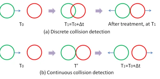
Collision detection can be classified into two types, discrete collision detection and continuous collision detection. For discrete collision detection, we do not consider the movement trajectories of objects. The cost of computation is lower, and it is faster than continuous collision detection. But some collisions may be missed, and objects may pass through each other within a frame. Therefore, discrete collision detection is inaccurate. For continuous collision detection, the movement trajectories of objects are considered. We interpolate the movement trajectories of objects between two frames. If the time step of the simulation between two frames is smaller, we can obtain more accurate contact time of two colliding objects. But the cost of computation is higher.
We illustrate the two types of collision detection in Figure 1.1: (a) discrete collision detection, and (b) continuous collision detection. In Figure 1.1(a), the green ball is moving toward the red ball at time T0. After a time step, we can obtain that the green ball and
the red ball are overlapping at time T1 by performing collision detection. Appropriate
treatment will be performed for the two balls at time T1. In fact, the collision has occurred
within the time interval [T0, T1]. In Figure 1.1(b), the green ball is moving toward the
red ball at time T0. We compute the movement trajectory of the green ball by using its
movement direction and velocity, and detect the collision between the two balls at time
Figure 1.1: Two types of collision detection. Let ∆t be the time step. treatment at time T′.
Collision detection between different objects is called inter-object collision detection. However, collision detection for an object itself is called intra(self)-object collision detec-tion. For rigid objects, suppose that they are independent, and there is no collision between themselves and the objects in the beginning. They may collide with or penetrate each other when moving. For deformable objects, such as cloth, collision occurs not only between the objects but also themselves. Therefore, self-collision detection should be handled for deformable objects. The computation of collision detection is quite expensive. A lot of techniques are developed to improve the performance of collision detection.
We can employ acceleration structures of objects to improve the performance of col-lision detection, such as bounding volume hierarchies (BVH). Each triangle is bounded by a bounding volume, and the acceleration structure is constructed by a top-down or a bottom-up manner. A leaf node of the BVH only contains a triangle. At the beginning of collision detection, we perform traversal for the BVHs of every two objects. The process of traversal is executed recursively by performing overlap tests of the bounding volumes until a pair of leaf nodes is reached. After that, we get a set of triangle pairs, called po-tentially colliding pairs. Finally, we perform elementary tests for the popo-tentially colliding pairs to obtain the actual colliding triangle pairs.
1.1
Motivation
Nowadays, computer graphics and animation are widely applied in video games, movies, mobile products, and smart phones. Collision detection is a primary technique to simulate activity of objects. And the performance of collision detection should be not only accurate but also interactive. In this thesis, our focus is on continuous self-collision detection for deformable objects. The deformable objects are cloth, such as clothes worn on a character. For cloth, there may be numerous self-collisions. Hence, the computation is quite expensive, and it is a challenge to improve the performance of self-collision de-tection for cloth. On the other hand, the development of graphics processing units (GPUs) is rapid. GPUs are very suitable for computation of vectors in computer graphics. In ad-dition, GPUs are employed for general purpose computation in recent years. Therefore, we employ GPUs to deal with a large number of computation of self-collision detection.
1.2
Overview
The main problem of self-collision is the high cost in checking the adjacent triangles. In fact, most adjacent triangles do not collide with each other. For the traditional method [VMT94], they compute normal cones and perform contour tests. A model is divided into several regular patches with hierarchical structures. The normal vectors of all triangles are bounded in each patch by computing a normal cone during the simulation phase. In the procedure, a lot of vectors and normalization are computed and the normal cones are bottom-up updated by merging the patches. Finally, contour tests are performed to check whether or not the model is self-collision free. Tang et al. [TCYM09] proposed a method to compute tightly bounded normal cones. However, the cost of normal cones computation is quite large due to computing additional vectors and normalization.
Hence, we want to eliminate the computation of normal cones and contour tests. We propose a novel view-based approach to perform continuous self-collision detection. Our method can be applied to deformable manifold triangle meshes, and we neither compute normal cones nor perform contour tests. Objects are determined whether or not they are
self-collision free by performing view tests. View tests are performed for all triangles by calculating dot products of the face normal vectors and the view-based vectors according to the view primitive and the triangles. The cost of performing view tests is much lower than computing the normal cones and performing contour tests. Our approach is suitable for column-liked models, such as dresses, pants, and shirts. In addition, the deformable objects should be closed. For unclosed triangle meshes, we can add some ghost triangles to enclose the boundaries. All edges are shared by two adjacent triangles for closed meshes. For unclosed meshes, there are some edges which only attach to one triangle. So, we can extract the boundary edges and generate the ghost triangles.
The view-based approach mainly has four steps, including view tests, boundary han-dling, traversal, and elementary tests. In the step of view tests, a deformable object is divided into several view sets based on their orientation related to a view primitive. The view primitive should be put inside the deformable object in the beginning, and we as-sume that it does not penetrate the deformable object during the simulation. All triangles of the deformable object are classified into three types include positive orientation, nega-tive orientation, and violation. For closed meshes, the triangles can be posinega-tively oriented and negatively oriented. For unclosed meshes, the triangles can be positively oriented, negatively oriented, and violated. If all triangles of an object are positively oriented, then the object is self-collision free. Otherwise, further checks should be performed for certain pairs of the view sets.
After performing view tests, traversal is performed to collect potentially colliding triangle pairs based on negatively oriented triangles and violated triangles. If the number of negatively oriented and violated triangles is few, the cost of performing traversal for them is low. Finally, elementary tests are performed for the potentially colliding pairs.
In recent years, the techniques of GPUs are getting mature and popular. Parallel computing is employed massively in computer graphics. Actually, our view-based ap-proach is suitable to be performed in parallel on GPUs. We use GPUs to accelerate our system with Compute Unified Device Architecture (CUDA). We evaluate our view-based approach with other methods. Our approach on CPUs outperforms other traditional
meth-ods, such as the approaches based on AABB [vdB99], K-DOP [KHM+98, MKE03], and
ICCD [TCYM09]. Besides, our approach implemented on GPUs is 12 times faster than the one on CPUs on average.
1.3
Contribution
Our major contributions of the thesis are described as follows.
1. A novel view-based approach for continuous self-collision detection with lower computation is proposed.
2. Partial BVHs for all kinds of view sets are employed to perform traversal. We do not construct new BVHs for the view sets but mark the nodes of the original BVH to ob-tain the partial BVHs. The cost of marking nodes is low, and the cost of performing traversal for these partial BVHs is low.
3. The view-based approach is implemented on GPUs with CUDA. We implement two versions: CPUs and GPUs.
4. It is easy to implement the view-based approach on both CPUs and GPUs. The concept of the view-based approach is simple and straightforward. A deformable object is divided into several view sets by performing view tests with computation of dot products.
5. Self-collision detection with triangle-based traversal is performed on GPUs. The de-gree of parallelism for performing traversal is higher with the triangle-based method. In other words, traversal is performed based on each triangle on GPUs.
6. The view-based approach is suitable for different kinds of models. Deformable objects are most suitable for column-liked objects, such as dresses, pants, bags, and shirts. Besides, a piece of cloth, which can form a sphere-liked or a cube-liked region, is also suitable for the view-based approach.
7. If an object is determined to be self-collision free after performing view tests, traver-sal is not required to be performed and the computation is reduced significantly. 8. The performance of self-collision detection using the view-based approach is
ac-ceptable for an object with a lot of self-collision. We can extract a set of triangles from an object by performing view tests that self-collision occurs at these triangles. On CPUs, traversal is performed for the partial BVHs of the different view sets respectively. On GPUs, traversal is performed with the triangle-based method.
1.4
Organization
The remaining chapters of the thesis are organized as follows. Chapter 2 reports the related work about collision detection, including implementing on CPUs and on GPUs. We present our based approach in Chapter 3. Chapter 4 and 5 present the view-based algorithms and their implementations. Chapter 6 presents the experimental results and discussion. Finally, Chapter 7 presents the conclusion and future work.
Chapter 2
Related Work
Collision detection is an important technique in physics simulation. A comprehensive overview of collision detection for deformable objects can be found in the survey paper [TKH+05].
By a brute force method, we can perform self-collision detection for all triangle pairs of an object. If the number of triangles of an object is n, then we need to execute(n2) elementary tests of all triangle pairs. A lot of techniques can be employed to improve the performance of self-collision detection, including bounding volumes, spatial partition-ing methods, and image-based methods. Boundpartition-ing volume hierarchies are AABB trees [vdB99], OBB trees [GLM96], k-DOP [KHM+98], and Sphere [PG95]. By using BVH, it
reduces the checking of triangle pairs that collision does not happen. The method employ-ing BVH uses many boundemploy-ing volumes with different sizes to bound an object. The entire object is enclosed with the largest bounding volume. Then, the object is divided into two similar parts and each part is bounded by another bounding volume. This is performed recursively until one or some triangles are enclosed with a bounding volume. BVH forms a structure of a tree. We can obtain a set of triangle pairs that every two triangles of a pair collide with each other by traversing the tree. Spatial partitioning includes octree [BT95] and BSP [Mel00]. The concepts of spatial partitioning and BVH are the same. The way of spatial partitioning is to partition the space into regular grids that bound the objects. The image-based methods rasterize meshes to framebuffer. The framebuffer includes stencil,
color, and depth buffer [BW02] [KP03] [VSC01].
Volino et al. [VMT94] proposed a breakthrough method for discrete self-collision detection. Originally, there is a lot of collision detection in checking adjacent triangle pairs. In general, most of adjacent triangles do not collide with each other. They di-vided a deformable object into several regular patches by computing normal cones, and performed contour tests to eliminate the collision check between adjacent triangle pairs. Provot [Pro97] extended the methods to handle continuous self-collision detection. After that, [WB05] [TCYM09] further improved the methods.
Recently, many parallel approaches were proposed for collision detection. Tang et al. [TMT09] proposed a parallel approach for collision detection with deformable models. The method performed incremental hierarchical computations and the hierarchies were built and updated each frame on multi-core CPUs. Kim et al. [KHH+09] combined the
techniques of CPUs and GPUs to improve the performance of continuous collision detec-tion. The main idea of the method is that traversal for BVHs is performed on CPUs, and elementary processing is performed on GPUs.
Due to the architecture of GPUs, they are more suitable than CPUs for performing parallel computation. Lauterbach et al. [LMM10] proposed an approach for rigid or de-formable models. The method proposed by Lauterbach was to perform parallel computa-tion for building, updating, and traversal of the hierarchies. Liu [LHLK10] implemented collision detection for massive moving rigid models. It changed the approach of Sweep and Prune (SaP) to the one of parallel SaP. And it reduced the number of false positives by using spatial subdivisions. Tang et al. [TMLT11] proposed a novel stream registration method to compute the triangle pairs that can have collision. And it reduced the overhead of the memory by using the deferred front tracking method.
Govindaraju et al. [GRLM03] used the technique of visibility-based culling to find out a potential collision set (PCS), and two-pass rendering algorithm to find out the part of collision. Due to the accuracy of image-based methods is affected by the resolution of images, Govindaraju et al. [GKJ+05] combined the method [GRLM03] with the technique
detection for deformable triangle meshes. Allard et al. [AFC+10] computed layered depth
images on GPUs, and then used the information to handle the contacts of models.
In addition to physics simulation, collision detection is also used for motion planning. Pan et al. [PM11] implemented cluster and collision-packet traversal on GPUs to improve the performance of collision detection for motion planning.
Chapter 3
View-based Scheme
The main concept of the view-based approach is to divide all triangles of a deformable object into several view sets according to their orientation related to a view primitive. We classify the triangles into four view sets and three types, including positively oriented, negatively oriented, and violated. If all triangles of the object face the view primitive, i.e. they are positively oriented, then the object is self-collision free. Thus traversal does not be performed. Otherwise, self-collision detection is performed for certain pairs of the view sets.
We use a point and a line segment to be the view primitives. So, there are two view-based schemes. We introduce the view-point model and the view-line model at first, then explain how to perform view tests according to the different view primitives. After that, two kinds of view-based schemes are described in details. Finally, we discuss the dif-ferences between the view-based approach and the traditional approach, and between the view-point scheme and the view-line scheme.
3.1
View-based Models
We use two kinds of view primitives to determine the orientation of all triangles, including a point and a line segment. The view primitives are put inside the deformable object in the beginning. Besides, we assume that the view primitives do not penetrate the
deformable object during the simulation.
The view-based point model is demonstrated in Figure 3.1. Suppose that q is the view-based point, and it is put at the center of the model.
Figure 3.1: The view-based point model.
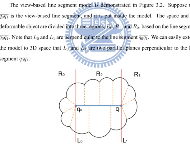
The view-based line segment model is demonstrated in Figure 3.2. Suppose that
q0q1 is the view-based line segment, and it is put inside the model. The space and the
deformable object are divided into three regions, R0, R1, and R2, based on the line segment
q0q1. Note that L0and L1are perpendicular to the line segment q0q1. We can easily extend
the model to 3D space that L0 and L1 are two parallel planes perpendicular to the line
segment q0q1.
Figure 3.2: The view-based line segment model.
The view-based point is called view-point, and the view-based line segment is called
3.2
View Tests with a Point
We determine the orientation of all triangles of a deformable object according to the view primitive by performing view tests. In this section, we introduce performing view tests with a view-point.
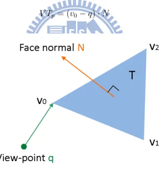
At a certain time
At first, we perform the view test of a triangle at a certain time. Assume that there is a triangle T (v0, v1, v2), and N = (v1− v0)× (v2− v0) is the normal vector of the triangle.
In addition, q is the view-point, as shown in Figure 3.3. We can choose any point of the triangle, for example vertex v0 is chosen, and obtain a vector v0− q. Then, the view test
is performed as follow.
V Tp = (v0− q) · N (3.1)
Figure 3.3: Triangle orientation determination with a view-point at a certain time.
Theorem 1. Suppose that there is a triangle T (v0, v1, v2), and N is the normal vector of
the triangle. q is a fixed view-point without intersecting with the triangle. If (v0−q)·N >
0, then for any point v of the triangle T , (v− q) · N is always greater than 0.
1. If∃ a point v′ such that (v′− q) · N = 0
⇒ v′− q and N are perpendicular
⇒ the triangle T and the point q are coplanar
This is a contradiction to (v0− q) · N > 0.
2. If∃ a point v′ such that (v′− q) · N < 0
Because the direction for normal vectors of all points of the triangle are the same, and (v0−q)·N > 0, there must be a point v′′of the triangle such that (v′′−q)·N = 0.
⇒ v′′− q and N are perpendicular
⇒ the triangle T and the point q are coplanar
This is a contradiction.
Based on that, the theorem is proved.
Corollary 1. Suppose that there is a triangle T (v0, v1, v2), and N is the normal vector of
the triangle. q is a fixed view-point without intersecting with the triangle. Then, for all points of the triangle T , the results of view tests are the same.
By Corollary 1, we can classify the type of a triangle by performing view tests with any point of the triangle according to the view-point. Then, by Theorem 1 and Equa-tion 3.1, we have three conclusions. For any point of a triangle T ,
• If V Tp > 0, then the triangle faces the view-point. • If V Tp < 0, then the triangle is back to the view-point. • If V Tp = 0, then the triangle is coplanar to the view-point.
Over a time interval
We perform the view test of a triangle over a time interval [0, ∆t], where ∆t is the time step of the simulation. During the simulation, all vertices move with linear velocities within a frame. Therefore, the position of a vertex v in [0, ∆t] should be vt = vbgn+ V t, where vbgnis the initial position of v, vtis the new position of v, V is the linear velocity of v, and t∈ [0, ∆t].
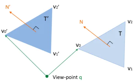
Assume that there is a triangle T (v0, v1, v2), and N = (v1 − v0)× (v2 − v0) is the
normal vector of the triangle in the beginning. After the time step ∆t, the triangle T moves to T′(v0′, v′1, v2′), and N′ is the normal vector of the triangle T′. In addition, q is the view-point, as shown in Figure 3.4. We can choose any point of the triangle T , for example vertex v0 is chosen, and perform the view test as follow.
V Tp(t) = v0(t)· N(t) (3.2)
V Tp(t) is a cubic function in the time domain, N (t) is the time normal vector of the triangle
T with quadratic form in the time domain, and v0(t) is a linear function in the time domain.
Hence, we want to compute v0(t) and N (t). Suppose that the velocities of vertices
v0, v1, and v2in [0, ∆t] are V0, V1, and V2. As mentioned above, the position of v0, v1, and
v2 at a certain time in [0, ∆t] are
vt0 = v0+ V0· t, t ∈ [0, ∆t]
vt1 = v1+ V1· t, t ∈ [0, ∆t]
vt2 = v2+ V2· t, t ∈ [0, ∆t]
• V1(t) and v2(t) are similar to the result of v0(t).
v0(t) = (v0− q) + ((v0t− q) − (v0− q)) = (v0− q) + ((v0+ V0· t − q) − (v0− q)) = (v0− q) + ((v0− q) + V0· t − (v0− q)) = (v0− q) + V0· t • Let Bs = v1− v0, Bt= V1− V0, Cs= v2− v0, Ct= V2− V0. N (t) = (v1t− v0t)× (vt2− v0t) = ((v1+ V1· t) − (v0+ V0· t)) × ((v2+ V2· t) − (v0+ V0· t)) = ((v1− v0) + (V1− V0)· t) × ((v2− v0) + (V2− V0)· t) = (Bs+ Bt· t) × (Cs+ Ct· t) = (Bs× Ct)· t2+ (Bt× Cs+ Bs× Ct)· t + Bs× Cs
Figure 3.4: Triangle orientation determination with a view-point over a time interval.
Theorem 2. Suppose that there is a triangle T , which moves from (v0, v1, v2) to (v′0, v1′, v2′)
in [0, ∆t], and N (t) is the time normal vector of the triangle T . q is a fixed view-point without intersecting with and passing through the triangle T in [0, ∆t]. If v0(t)·N(t) > 0,
then for any point v of the triangle, v(t)· N(t) is always greater than 0 in [0, ∆t]. Proof. We prove it as follows.
If the triangle T does not pass through the view-point q, and v0(t)· N(t) > 0, then the
triangle T always faces the view-point q in [0, ∆t]. By Theorem 1, all the vertices of the triangle face the view-point q. Therefore, for any point v of the triangle, v(t)· N(t) is always greater than 0 in [0, ∆t].
Corollary 2. Suppose that there is a triangle T , which moves from (v0, v1, v2) to (v′0, v1′, v2′)
in [0, ∆t], and N (t) is the time normal vector of the triangle T . q is a fixed view-point without intersecting with and passing through the triangle T in [0, ∆t]. Then, for all points of the triangle T , the results of view tests are the same in [0, ∆t].
By Corollary 2, we can classify the type of a triangle by performing view tests with any point of the triangle over a time interval according to the view-point. Then, by The-orem 2 and Equation 3.2, we have three conclusions. For any point of a triangle T in [0, ∆t],
set V+
p .
• If V Tp(t) < 0, then the triangle is back to the view-point, and it is assigned to the view set Vp−.
• If V Tp(t) contains both positive and negative values, then the triangle is coplanar to the view-point at a certain time in [0, ∆t], and it is assigned to the view set Vp0.
3.3
View Tests with a Line Segment
In this section, we introduce performing view tests with a view-line.
Figure 3.5: Triangle orientation determination with a view-line at a certain time.
At a certain time
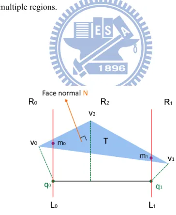
At first, we perform the view test of a triangle at a certain time. Assume that there is a triangle T (v0, v1, v2), and N = (v1− v0)× (v2− v0) is the normal vector of the triangle.
In addition, q0q1is the view-line, as shown in Figure 3.5. We can choose a vertex v of the
triangle T and obtain a vector v− vp, where vp is the check point on the view-line q0q1.
Then, the view test is performed as follow.
vp has three types according to the location of v.
1. If v ∈ R0, then vp = q0.
2. If v ∈ R1, then vp = q1.
3. If v ∈ R2, then vp = the projective point of v on the view-line q0q1.
Therefore, view tests based on the view-point model and the view-line model are different. For the view-line model, we divide space and deformable objects into three regions, and the check points are different with respect to different vertices. Hence, before performing view tests of a triangle, we determine the regions for three vertices of a triangle. For a vertex v of the triangle T , the projective point of v on the view-line q0q1 should
be vp = q0+ u× (q1− q0). −−→ q0q1 · (vp− v) = (q1 − q0)· (vp − v) = (q1 − q0)· ((q0+ u× (q1− q0))− v) = (q1 − q0)· (q0− v) + u × ((q1− q0)· (q1− q0)) = 0 ⇒ u = (v− q0)· (q1− q0) (q1− q0)· (q1− q0)
Then, we can determine the regions for the vertex v based on the value of u. • If u < 0, then v ∈ R0.
• If u > 1, then v ∈ R1.
• If u ∈ [0, 1], then v ∈ R2.
Theorem 3. Suppose that there is a triangle T (v0, v1, v2), and N is the normal vector of
the triangle. q0q1 is a fixed view-line without intersecting with the triangle. Then, for all
vertices of the triangle T , the results of view tests are the same. Proof. We prove it as follows.
• Case 1: For any two vertices, if they are in the same region, R0 or R1, then it is
proved by Corollary 1.
• Case 2: For any two vertices, if they are in the same region, R2, then suppose that
v0 and v1 are chosen, and v0p and v1pare the projective points of v0 and v1 on the
view-line q0q1.
A = (v0− v0p)· N
B = (v1− v1p)· N
C = (v0 − v1p)· N
D = (v1− v0p)· N
By Corollary 1, we have the following results.
The results of A and D are the same according to the fixed point v0p.
The results of B and C are the same according to the fixed point v1p.
The results of A and C are the same according to the fixed point v0.
The results of B and D are the same according to the fixed point v1.
Therefore, the results of V Tv0 = (v0− v0p)· N and V Tv1 = (v1− v1p)· N are the same.
• Case 3: For any two vertices, if one vertex belongs to R0 and the other belongs to
R2, then suppose that v0 and v1 are chosen that v0 ∈ R0 and v1 ∈ R2, as shown in
Figure 3.6. We can find a point m of the triangle that the projective point of m on the view-line q0q1 is q0. The results of V Tv0 and V Tm are the same by case1. The results of V Tm and V Tv1 are the same by case2. So, the results of V Tv0 and V Tv1 are the same.
• case4: For any two vertices, if one vertex belongs to R1, and the other belongs to
R2, then the result is similar to case3.
• case5: For any two vertices, if one vertex belongs to R0 and the other belongs to
R1, then suppose that v0 and v1 are chosen that v0 ∈ R0 and v1 ∈ R1, as shown in
Figure 3.6: Triangle orientation determination with a view-line at a certain time when the triangle lies in multiple regions.
Figure 3.7: Triangle orientation determination with a view-line at a certain time when the triangle lies in multiple regions.
the projective points of m0 and m1on the view-line q0q1are q0 and q1. The results
of V Tv0 and V Tm0 are the same, and the results of V Tm1 and V Tv1 are the same by case1. The results of V Tm0 and V Tm1 are the same by case2. So, the results of
V Tv0 and V Tv1 are the same.
According to the above results, it is proved. Hence, for all vertices of the triangle T , the results of view tests are the same.
Therefore, we can classify the type of a triangle by performing view tests with any point of the triangle according to the view-line. In addition, the chosen vertex belongs to only one region at a certain time, so view tests are performed for just one time. By Theorem 3 and Equation 3.3, we have three conclusions. For any point of a triangle T ,
• If V Tl > 0, then the triangle faces the view-line.
• If V Tl < 0, then the triangle is back to the view-line.
• If V Tl = 0, then the triangle is coplanar to the view-line.
Over a time interval
Next, we perform view tests of a triangle over a time interval [0, ∆t], where ∆t is the time step of the simulation. During the simulation, all vertices move with linear velocities within a frame. Therefore, the position of a vertex v at a certain time in [0, ∆t] should be
vt= v
bgn+ V t, where vbgnis the initial position of v, vtis the new position of v, V is the linear velocity of v, and t∈ [0, ∆t].
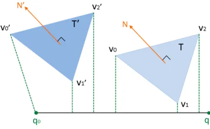
Assume that there is a triangle T (v0, v1, v2) and N = (v1 − v0)× (v2 − v0) is the
normal vector of the triangle in the beginning. After the time step ∆t, the triangle moves to T′(v0′, v1′, v2′), and N′ is the normal vector of the triangle T′. In addition, q0q1 is the
view-line, as shown in Figure 3.8.
Before performing view tests of a triangle, we determine the regions that the triangle belongs to because the triangle can spread and move across multiple regions in [0, ∆t]. The regions for a triangle are determined by its three vertices. We compute the regions
Figure 3.8: Triangle orientation determination with a view-line over a time interval when the triangle moves across multiple regions.
for three vertices, then the regions for the triangle are the union of the regions for its three vertices.
Suppose that there is a vertex of the triangle, which moves from v to v′ in [0, ∆t]. Then, the projective points of v and v′ on the view-line q0q1 should be vp = q0 + ubgn× (q1−q0) and vp′ = q0+ uend×(q1−q0). Because the vertices move linearly, [ubgn, uend] is also linear. We can determine the regions that the vertices move across in [0, ∆t] according to the values of ubgnand uend.
Let Rv0, Rv1, and Rv2 are the regions that the three vertices v0, v1, and v2move across in [0, ∆t]. So, the regions for the triangle are Rv0∪ Rv1 ∪ Rv2. Note that the check points are different based on different vertices of the triangle. Actually, view tests are performed based on the vertices. Suppose that v is one of the vertices of the triangle T . Then, the view test is performed as follow.
V Tl(t) = v(t)· N(t) (3.4)
V Tl(t) is a cubic function in the time domain, N (t) is the time normal vector of triangle T with quadratic form in the time domain, and v(t) is a linear function in the time domain for the vector variation from the vertex to the check points in [0, ∆t]. Note that we compute v(t) separately according to the region for the vertex. For example, if a vertex v
moves from R0to R2in [0, ∆t], then the check point is variable. So, the function of vector
variation from the vertex to the check point is not linear. We should compute n kinds of
v(t), where n is the number of regions for the vertex in [0, ∆t].
Suppose that the velocities of vertices v0, v1, and v2 in [0, ∆t] are V0, V1, and V2. As
mentioned above, the positions of v0, v1, and v2at a certain time in [0, ∆t] are
vt0 = v0+ V0· t, t ∈ [0, ∆t]
vt1 = v1+ V1· t, t ∈ [0, ∆t]
vt2 = v2+ V2· t, t ∈ [0, ∆t]
Then, v(t) and N (t) are computed as follows.
• For any vertex v, v moves across R0 or R1in [0, ∆t].
v(t) = (v− vq) + ((vt− vq)− (v − vq)) = (v− vq) + ((v + V · t − vq)− (v − vq)) = (v− vq) + ((v− vq) + V · t − (v − vq)) = (v− vq) + V · t
vqis q0or q1 according to the location of v.
• For any vertex v, v moves across R2 in [0, ∆t].
v(t) = (v− vq0) + ((vt− vqt)− (v − vq0)) = (v− vq0) + ((v + V · t − vqt)− (v − vq0)) = (v− vq0) + (v− vqt) + V · t − (v − vq0) = (v− vqt) + V · t
vq0 is the projective point of v in the beginning, and vqtis the projective point of v at a certain time in [0, ∆t].
• Let Bs = v1− v0, Bt= V1− V0, Cs= v2− v0, Ct= V2− V0 N (t) = (v1t− v0t)× (vt2− v0t) = ((v1+ V1· t) − (v0+ V0· t)) × ((v2+ V2· t) − (v0+ V0· t)) = ((v1− v0) + (V1− V0)· t) × ((v2− v0) + (V2− V0)· t) = (Bs+ Bt· t) × (Cs+ Ct· t) = (Bs× Ct)t2+ (Bt× Cs+ Bs× Ct)t + Bs× Cs
Theorem 4. Suppose that there is a triangle T , which moves from (v0, v1, v2) to (v′0, v1′, v2′),
and N (t) is the time normal vector of the triangle T . q0q1is a fixed view-line without
in-tersecting with and penetrating the triangle in [0, ∆t]. Then, for all vertices of the triangle T , the results of view tests are the same in [0, ∆t].
Proof. We prove it as follows.
• Case 1: For any two vertices, if they move in the same region in [0, ∆t], then the results of view tests are always the same by Theorem 3.
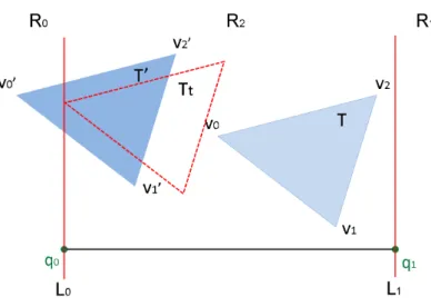
• Case 2: For any two vertices, if they move across multiple regions in [0, ∆t], the proof is described as follows. For example, in Figure 3.9, v0moves from R2to R0,
and v1 and v2 move inside R2 in [0, ∆t]. Suppose that the triangle T moves to Tt at time t, where t ∈ [0, ∆t]. In [0, t], all vertices move in the same region and the results of view tests are the same by Theorem 3. On the other hand, in (t, ∆t], We can always find a point mtthat the projective point of mton the view-line q0q1 is
q0. So, the results of view tests of v0 are equal to the point mtin (t, ∆t]. And the results of view tests of v1and v2are equal to the point mtin (t, ∆t]. Therefore, the results of view tests of v0, v1, and v2 are the same.
By Case 1 and Case 2, it is proved. Hence, for all vertices of the triangle T , the results of view tests are the same in [0, ∆t].
Therefore, we can classify the type of a triangle by performing view tests with any point of the triangle over a time interval according to the view-line. View tests are per-formed for nr times, where nr is the number of regions that the chosen vertex moves
Figure 3.9: Triangle orientation determination with a view-line over a time interval when the triangle moves across multiple regions.
across in [0, ∆t]. By Theorem 4 and Equation 3.4, we have three conclusions. Suppose that the result of view tests for a triangle T is V Tl(t) = ∪V Tli(t), where V Tli(t) are the results of view tests according to region Ri, i = 0, ..., n− 1, and 1 ≤ n ≤ 3. For any point of a triangle T in [0, ∆t],
• If ∀V Tli(t) > 0, then V Tl(t) > 0. So, the triangle faces the view-line, and it is assigned to the view set Vl+.
• If∀V Tli(t) < 0, then V Tl(t) < 0. So, the triangle is back to the view-line, and it is assigned to the view set Vl−.
• If V Tli(t) contain both positive and negative values, then the triangle is coplanar to the view-line at a certain time in [0, ∆t], and it is assigned to the view set V0
l .
3.4
View-based Self-Collision Detection
If a deformable object has self-collision, then there are some properties for the trian-gles at the colliding position. Let's take a look on a 2D closed curve, for example. Suppose that there is a 2D closed curve, and there is no self-intersection. In fact, the curve is called a Jordan curve, as shown in Figure 3.10. By the Jordan curve theorem, the curve divides
the 2D space into two regions, an interior region and an exterior region. For example, in Figure 3.10, the interior region is indicated by green color, and the exterior region is indicated by blue color.
Figure 3.10: A 2D closed curve with a ray shot outward.
Now, we shoot a ray from a fixed point P in the interior region to any point in the exterior region, as shown in Figure 3.10. We can observe that the ray must intersect with the curve for odd number of times. Initially, the ray lies in the interior region. After the first time the ray intersects with the curve, the ray lies in the exterior region. However, when the ray intersects with the curve again, the ray must lie in the interior region. In short, after the ray intersecting with the curve, the ray lies in the different region.
Suppose that the normal vectors of the curve point to the exterior region. And there is a ray R with direction d shot from the point P to the exterior region and intersected with the curve at P0, P1, and P2 orderly, as shown in Figure 3.10. P0 is the first intersection
point. In this case, d· NP0 ≥ 0, where NP0 is the normal vector of the point P0. So, we can determine that the point P0 faces the point P . Next, P1 is the second intersection
point. In this case, d· NP1 ≤ 0, where NP1 is the normal vector of the point P1. So we can determine that the point P1 is back to the point P . Finally, P2 is the third intersection
point. In this case, d· NP2 ≥ 0 again, where NP2 is the normal vector of the point P2. So, we can determine that the point P2 faces the point P .
For a 2D closed curve with no self-intersection, we can now conclude that if a ray shoots from a point P inside the curve and intersects with some points on the curve. When
an intersection occurs between the ray and the curve, the regions that the ray lies and the orientation of the intersection points according to P are opposite.
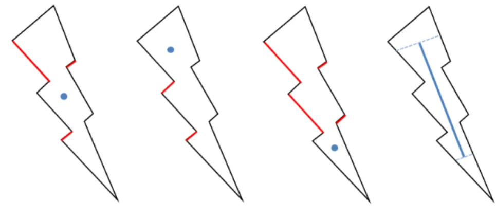
Now, for a 2D closed curve with self-intersection, suppose that the colliding point is called pc. A ray is shot from the point P in the interior region to pc, as shown in Figure 3.11. At the colliding position, the ray should intersect with the curve for greater than or equal to two times. Therefore, there are at least two points that one faces P and another is back to P at the colliding position. In addition, there is a special case. At the colliding position, the normal vectors of the points are perpendicular to the direction of the ray, i.e. d·Ni = 0, where i is the number of points at the colliding position.
Figure 3.11: 2D closed curves with self-intersection.
Theorem 5. Suppose that there is a 2D closed curve with self-intersection. A point P is put in the interior region of the curve. Then, at the colliding position, there are two points px and py that (d· Nx)· (d · Ny) < 0 or both Nxand Ny are perpendicular to d, where d
is the direction of a ray shot from the point P to the exterior region of the curve, and Nx
and Ny are the normal vectors of pxand py.
Proof. If we shoot a ray from the point P to the colliding position, then there are two
points at least at the colliding position. By the Jordan curve theorem, the location, which the ray passes through, should be change when the ray intersects with the curve, and the orientation should be opposite for any two consecutive intersection points. Now, we have two points, suppose they are pxand py, at least at the colliding position, so, the orientation
of px and py are opposite according to P , and (d · Nx)· (d · Ny) < 0. Besides, for the special case, Both Nxand Ny can be perpendicular to d.
We can extend the results to a 2D closed curve with a line segment in the interior region. We divide the space and the curve into three regions. Originally, we create a ray shot from the point P in the interior region to the exterior region. Now, we create a ray shot from the check point on the line segment to the curve. The check point is determined by the region that the curve belongs to. We can further extend the results to 3D closed triangle meshes with a point or a line segment inside the meshes.
Corollary 3. Suppose that there is a 3D closed model with triangle meshes, and a point q lies inside the meshes. If self-collision occurs, then there are at least two triangles at the colliding position that one faces the point q, and another is back to the point q, or the normal vectors of these two triangles are both perpendicular to the vector from q to themselves.
Corollary 4. Suppose that there is a 3D closed model with triangle meshes, and a line segment q0q1lies inside the meshes. If self-collision occurs, then there are at least two
tri-angles at the colliding position that one faces the line segment q0q1, and another is back to
the line segment q0q1, or the normal vectors of these two triangles are both perpendicular
to the vector from the check points to themselves.
Handling unclosed meshes
The view-based approach is suitable for closed meshes. For unclosed meshes, there are some modification of the view-based approach. For example, for a 2D unclosed curve, the boundaries of the curve may roll, as shown in Figure 3.12. We can observe that the edges a and b both face the view-point q, and they collide with each other at point pc. This is a contradiction to Theorem 5. So, we collect the edges which are determined to be violated. Similarly, for a 3D model, we collect the triangles which do not conform to Corollary 3 and 4. These triangles are called violated triangles.
Figure 3.12: A 2D unclosed curve with self-intersection.
Figure 3.13: An example of handling unclosed objects.
For example, suppose that there is a 2D unclosed curve with a gap in the beginning, as shown in Figure 3.13. The curve is composed of several line segments. We create a ghost edge to enclose the gap, which is indicated by green color. The edges, which collide with the ghost edge, are indicated by red color. We collect these red edges into a violated view set Vv. Finally, the view set Vv contains the red edges and orange edges. In other words, Vvcontains the edges which overlap with or pass through the ghost edge.
3.5
View-Point Scheme
For the view-point scheme, we divide the triangles of a deformable object into three view sets at first, including V+
p , Vp−, and Vp0. In addition, there is an additional view set,
Vv
p, for unclosed meshes. We classify the types of all triangles according to the method de-scribed in section 3.2. For all triangles, view tests are performed by V Tp(t) = v(t)· N(t), where v(t) is a linear function in the time domain according to the movement trajectory of one of the vertices, and N(t) is the time normal vector with quadratic form in the time domain.
Triangles in V+
p are determined to be positively oriented. Triangles in Vp−and Vp0are determined to be negatively oriented. Triangles in Vpv are determined to be violated.
Theorem 6. Suppose that there is a deformable object Mcand a point q. The
view-point is put inside the object in the beginning, and we assume that the view-view-point does not pass through the deformable object during the simulation. If all triangles of Mcare
positively oriented according to the view-point in [0, ∆t], then Mcis self-collision free.
Proof. We prove it as follows.
If self-collision occurs at a certain time in [0, ∆t]. Then, at the colliding position, there are two triangles at least that one faces the view-point q, and another is back to the view-point
q, or the normal vectors of these two triangles are both perpendicular to the vectors from
the view-point q to themselves. If a triangle is back to the view-point, then V Tp(t) < 0. If a triangle is coplanar to the view-point, then V Tp(t) = 0. This is a contradiction because the results of view tests of all triangles are V Tp(t) > 0. So, if all triangles of Mc are positively oriented according to the view-point q, then Mcis self-collision free.
If a deformable object is determined to be self-collision free after performing view tests, then we do not perform traversal. Otherwise, we perform traversal for certain pairs of the view sets. By Corollary 3, for closed meshes, we observe that triangles in V+
p and Vp−may collide with each other. And triangles in Vp0 may collide with all triangles. Because that, for any triangle T in V0
p, when T faces the view point at a certain time, it may collide with triangles which are back to the view point. When T is coplanar to the view point at a certain time, it may collide with other coplanar triangles. When T is back to the view point at a certain time, it may collide with the triangles which face the view point. Actually, there are several triangles at a colliding position, and two positively oriented triangles may collide with each other, or a positively oriented triangle may collide with a coplanar triangle. We just need to detect the collision with two triangles but not all colliding triangle pairs at the colliding position. We have proved that there must be two triangles at least that one faces the view point, and another is back to the view point, or the normal vectors are both perpendicular to the vectors from the view point to themselves.
So, if a deformable object is not self-collision free, we perform traversal for the following pairs to collect potentially colliding pairs.
• (V+
p , Vp−) • (U, V0
p)
U is the union set of all triangles of the deformable object. For unclosed meshes, after
performing view tests, we divide all triangles into three view sets. After that, violated triangles are collected by performing boundary handling. We pick out violated triangles from the three view sets. In other words, violated triangles are special and independent, and they may collide with all triangles. We perform further checks for the following pairs to collect potentially colliding pairs.
• (Vp+′, Vp−′) • (U′, V0 p ′) • (U, Vpv) V+ p ′ = V+ p − Vpv, Vp− ′ = V− p − Vpv, Vp0 ′ = V0
p − Vpv, and U′ = U − Vpv. Note that
V+ p ′ ∩ V− p ′∩ V0 p ′∩ Vv p = ϕ.
The view-point scheme
1. Compute a point inside the deformable object Mcin the preprocessing stage.
2. Divide all triangles of the deformable object into three view sets, including V+
p , Vp−, and Vp0. For unclosed meshes, there is an additional view set, Vpv.
3. If all triangles are in the set V+
p , then the deformable object Mcis self-collision free. 4. Otherwise, we need to perform further checks for the pairs of (V+
p , Vp−) and (U, Vp0). For unclosed meshes, we need to perform further checks for the pairs of (Vp+′, Vp−′), (U′, V0
p
′), and (U, Vv p).
3.6
View-Line Scheme
For the view-line scheme, we divide the triangles of a deformable object into three view sets at first, including Vp+, Vp−, and Vp0. In addition, there is an additional view set,
Vv
l , for unclosed meshes. We classify the types of all triangles according to the method described in section 3.3. For all triangle, view tests are performed by V Tl(t) = v(t)·N(t), where v(t) is a linear function in the time domain according to the movement trajectory of one of the vertices, and N(t) is the time normal vector with quadratic form in the time domain.
Triangles in Vl+are determined to be positively oriented. Triangles in Vl−and Vl0are determined to be negatively oriented. Triangles in Vlv are determined to be violated.
Theorem 7. Suppose that there is a deformable object Mc and a view-line q0q1. The
space and the object are divided into three regions, R0, R1, and R2. The view-line is put
inside the object in the beginning, and we assume that the view-line does not penetrate the deformable object during the simulation. If all triangles of Mcare positively oriented
according to the view-line in [0, ∆t], then Mcis self-collision free.
Proof. We sketch our proof as follows.
Suppose that we divide the triangles into three sets, S0, S1, and S2 according to the three
regions, R0, R1, and R2. We can show the triangles in each set Si are self-collision free. Then, we can show that it is collision free between two sets of the sets.
Consider that there are triangles in one set, which have collision. Then assume that these two triangles are T0 and T1. We can show that this is not possible as there must be
the third triangle which is negatively oriented with respect to the view-line according to the Jordan curve theorem. This is a contradiction to our assumption.
Consider that there are two triangles collide between two sets. Assume that these two triangles are T0 and T1. Then T0 is a triangle in one set, and T1 is a triangle in another
set. However, T0and T1must also belong to the same set as there is at least one vertex of
a triangle belong to both set; otherwise, these two triangles cannot collide. However, we have already shown that it is collision free in a set.
If a deformable object is self-collision free, then we do not perform traversal. Other-wise, by Corollary 4, we perform further checks for the following pairs to collect poten-tially colliding pairs.
• (Vl+, Vl−) • (U, Vl0)
U is the union set of all triangles of the deformable object. For unclosed meshes, we
perform further checks for the following pairs to collect potentially colliding pairs. • (Vl+′, Vl−′) • (U′, V0 l ′) • (U, Vlv) Vl+′ = Vl+ − Vv l , Vl− ′ = V− l − V v l , Vl0 ′ = V0
l − Vlv, and U′ = U − Vlv. Note that
Vl+′ ∩ Vl−′∩ V0
l
′∩ Vv l = ϕ.
The view-line scheme
1. Compute a line segment inside the deformable object Mcin the preprocessing stage.
2. Divide all triangles of the deformable object into three view sets, including Vl+, Vl−, and Vl0. For unclosed meshes, there is an additional view set, Vlv.
3. If all triangles are in the set Vl+, then the deformable object Mcis self-collision free. 4. Otherwise, we need to perform further checks for the pairs (Vl+, Vl−) and (U, V0
l ). For unclosed meshes, we need to perform further checks for the pairs of (Vl+′, Vl−′), (U′, V0
l
′), and (U, Vv l ).