基於最佳權重預測法之九宮格式差值擴張資訊隱藏技術

全文

(1)國立高雄大學資訊工程學系碩士論文. 基於最佳權重預測法之九宮格式差值擴張資訊隱藏技術 Difference Expansion of Data Hiding Based on The Prediction of Optimal Weights of 3×3 Box Filter. 研究生：林坪亨撰指導教授：陳建源博士. 中華民國一百年六月.

(2) 基於最佳權重預測法之九宮格式差值擴張資訊隱藏技術指導教授：陳建源博士（教授）國立高雄大學資訊工程學系. 學生：林坪亨國立高雄大學資訊工程學系. 摘要. 在本研究中，我們提出新的演算法來增強差值擴張的偽裝影像品質。我們的演算法引入了最佳化權重及九宮格式，來改良原差值擴張資訊隱藏技術。根據九宮格式的特性，可偵測更多方向的變動，可適用於複雜的影像。而最佳化權重的設定，使預測差值的產生盡可能朝最多差值為零的個數去收斂，使得偽裝影像保持低失真度。實驗結果顯示，在一樣的嵌入量的前提下與其他方法相比，針對複雜影像，平均 PSNR 增加 6.89%。因此，我們的方法有利於將機密資訊藏入複雜影像的同時，亦能兼顧偽裝影像的品質。. 關鍵詞：最佳化權重、九宮格式、差值擴張。.

(3) Difference Expansion of Data Hiding Based on The Prediction of Optimal Weights of 3×3 Box Filter Advisor(s): Dr.(Professor) Chien-Yuan Chen Department of Computer Science and Information Engineering National University of Kaohsiung. Student: Ping-Heng Lin Department of Computer Science and Information Engineering National University of Kaohsiung. ABSTRACT. In this research, we present a new method to improve the quality of stego image. We improve the difference expansion method by using optimal weights and 3×3 box filter. The 3×3 box filter is suitable for complicated image because 3×3 box filter can detect more direction of each pixel. The optimal weights keep high PSNR of the stego image because optimal weights generate more zero-difference. Experiment shows that our method arises 6.89% PSNR than the presented method for complicated image. Therefore, our method hide secret bits with high PSNR for the complicated image.. Keywords：Optimal Weight, 3×3 Box Filter, Difference Expansion.. ii.

(4) Content Content..................................................................................................................................... iii Content of Figure ......................................................................................................................iv Content of Table.........................................................................................................................v Acknowledgement ....................................................................................................................vi 1. Introduction ....................................................................................................................1 2. Related Work..................................................................................................................5 2.1 Use of Rhombus Pattern Prediction .......................................................................5 2.2 Use of Histogram Shift Scheme .............................................................................7 2.3 Use of Sorting ........................................................................................................7 2.4 Use of Overflow and Underflow Problem .............................................................8 2.4.1 Encoder Testing..........................................................................................8 2.4.2 Decoder Testing .........................................................................................9 2.5 Instance ..................................................................................................................9 2.5.1 Instance of Encoder..................................................................................10 2.5.2 Instance of Decoder .................................................................................11 3. Our method ..................................................................................................................14 3.1 3×3 Box Filter ......................................................................................................14 3.2 The Predictive Method of Optimal Weights ........................................................15 3.3 Local Varience .....................................................................................................18 3.4 Algorithm .............................................................................................................19 3.4.1 Definition of Symbols ..............................................................................19 3.4.2 Algorithm of Encoder ..............................................................................21 3.4.3 Instance of Encoder..................................................................................23 3.4.4 Definition before Decoder Algorithm ......................................................25 3.4.5 Algorithm of Decoder ..............................................................................25 3.4.6 Instance of Decoder .................................................................................27 4. Experiments and Discussion ........................................................................................29 5. Conclusion ...................................................................................................................34 References................................................................................................................................35. iii.

(5) Content of Figure Fig. 1. Prediction pattern............................................................................................................5 Fig. 2. Distribution of orignal image’s pixel............................................................................10 Fig. 3. Distribution of stego image’s pixel...............................................................................10 Fig. 4. Distribution of recovery image’s pixel. ........................................................................13 Fig. 5. 3×3 box filter. ...............................................................................................................14 Fig. 6. Distribution of orignal image’s pixel............................................................................23 Fig. 7. Distribution of stego image’s pixel...............................................................................23 Fig. 8. Distribution of recovery image’s pixel. ........................................................................28 Fig. 9. Experiment curve of Lena ............................................................................................30 Fig. 10. Experiment curve of Peppers......................................................................................30 Fig. 11. Experiment curve of Baboon ......................................................................................31 Fig. 12. Experiment curve of Boat...........................................................................................31 Fig. 13. Experiment curve of Airplane.....................................................................................32. iv.

(6) Content of Table Table 1. The encoder processing step by step..........................................................................11 Table 2. The decoder processing step by step..........................................................................12 Table 3. The encoder processing step by step..........................................................................24 Table 4. The decoder processing step by step..........................................................................27 Table 5. The five 512×512 grayscale images for experiment. .................................................29 Table 6. The enhanced ratio of average PSNR ........................................................................32. v.

(7) Acknowledgement 首先，我要先感謝指導老師陳建源教授這兩年來細心的指導，每一次的報告中，老師都能提出不一樣的見解，使我思考解決問題的各種不同可能，令研究不再枯燥乏味。老師雖然身兼主任，卻很肯花時間撥空與我討論，這令我十分的感激。接著，我也要感謝願意擔任我的口試委員的章定遠教授與吳俊興助理教授，兩位老師在口試中給的建議，不管是章老師對小細節的敏銳觀察，以及吳老師對實驗設計的假設，的確是使我論文趨於完備的方針。兩年的碩士生涯匆匆即逝，與實驗室的成員：鈺峰學長、筱凌學姐、宇哲、柏豪、昱瑄、能寅、士倫、俊欽，閒暇時的糾團吃飯、打球、跑團、嘴砲，如今歷歷在目，也推翻我以往對研究生不愛玩的刻板印象。最後，我要感謝我的母親以及一直支持我的父方親人，沒有你們的支持，我無法完成碩士學業。還有，我想感謝在天堂的父親，小時候我最討厭的科目是數學，是父親利用很多有趣的例子，令我迷途知返愛上數學。今天的我是接受多方的幫助才有今天的成就，以後我當飲水思源，幫助更多的人以回饋彼此，成就彼此，讓大家的生活都能進一步提昇。林坪亨 2011.07.26. vi.

(8) 1. Introduction Internet has become a new bridge of communication between people, as the maturity of network technology and the popularity of computer. On internet, the problems, such as network security and data protection, must be conquered when people pass message or multi-media. To solve the previous problems, scholars have proposed information hiding techniques [1, 2, 3, 4, 5, 6, 7, 8, 9, 10, 11]. The information hiding techniques hide secret data in a cover image to generate a stego image. If the cover image could be reconstructed from the stego image, we call this reversible technique; otherwise, the technique is irreversible. Because reversible information hiding techniques support multi-layer embedding, many experts and scholars paid attention on these techniques. Reversible information hiding techniques can be roughly divided into three categories [9]: Histogram, Vector quantization, and Difference expansion. Because difference expansion method overcomes the other two methods with high payload (0.5bpp ~ 1bpp), many scholars presented the related study [1, 2, 3, 4, 5, 7]. Difference expansion method was first proposed by Tian [1] in 2003. Tian's method divides the image into pairs of pixels, and then uses some pairs for hiding secret data. For each pair of pixels, we can generate two parameters, average and difference, to determine where we can embed secret data. Therefore, Tian's embedding capacity is at best 0.5 bpp(Celik et al. [10] is 0.35bpp at the same PSNR). However, Tian’s method needs a location map of large size. Without a location map, the decoder cannot fetch secret data exactly because we do not know which pairs were modified. Thus, how to reduce the size of the location map is one of the key goals in this field. The simple method aims at compressing 1.

(9) location map. And following scholars implement variant improvement on Tain’s method [1]. Alattar et al. [3] proposed a smaller location map method. Thodi et al. [4] proposed a novel difference generation method. Sachnev et al. proposed a sorting order method base on Kamstra et al.’s method [7]. Alattar [3] presented a cell concept to reduce the size of the location map. Alattar has defined one cell as triplet pixels to hide two bits. A cell is the unit of pixels in which the data will be embedded. Alattar’s location map covers all triplets instead of pairs. Thus, the uncompressed location map size is decreased from one-half of the image resolution (Tian’s method) to one-third of the resolution (for triplets). Obviously, Alattar’s method has advantages over Tian’s method, since the cell can hide data even if the location map is not compressed whereas it is not possible in Tian’s method. If the location map is compressed, Alattar’s method significantly outperforms Tian’s method. Thodi et al. [4] proposed a histogram shift method to reduce location map. Thodi et al. use a threshold to divde the histogram of predictive difference into two set, shift set and expansion set. Only in expansion set, we can embed secret bit. However, Thodi et al.’s method causes ambiguous problem when processing algorithm of decoder side. Because decoder does not know whether stego pixel is modified or not. To solve ambiguous problem, Thodi et al. implement a different location map. The location map is used Sachnev et al.’s predictive method to only record all ambiguous cells which can not be recoverable. The number of ambiguous cells is lower than the size of Tain’s location map. Sachnev et al. utilized sorting and prediction to present a reversible algorithm [5]. They enhanced Kamstra et al. [7]‘s sorting technique to process cells based on magnitude of local variances. And they also present a rhombus pattern’s predictive method which allows us to embed secret data in multilayer. Sorting predictive differences were used to embed more data into the image with less distortion. But Sachnev et al.’s predictive method just handle 2.

(10) horizontal and vertical directions. The Sachnev et al.’s predictive method’s property only suits smooth image. Lin et al. [6] presented 3×3 box filter to hide secrets in complicated image. Lin et al. [11] propose the 3×3 box filter to enhance Sachnev et al.’s method [5]. Lin et al. consider that rhombus pattern is not suitable for complicated image. Therefore, Lin et al. present the 3×3 box filter to improve rhombus pattern’s drawback. The 3×3 box filter has two advantage for difference expansion. First, 3×3 box filter makes the prediction more accurately (lower magnitude of difference ). Second, the pattern of 3×3 box filter influences the processing order, the lower magnitude of local variance gets the higher processing weight. So, Lin et al.’s method has higher capacity and lower distortion. Difference expansion losses its advantages when most predictive differences are not equivalent to zero. This drawback infers not only less capacity, but high distortion. It motivates us to present new data hiding method based on the prediction of optimal weights of 3×3 box filter. In this paper, we utilize Lin et al.’s method [6] to enhance predictive method by choosing neighbor pixels. Not only simple image but also complicated image is suited to prediction of Lin et al.’s method. Besides, we also propose a concept of optimal weight to gernerate more accurate. The optimal weights are the dominated constants which make the linear combination between neighbor pixels and original pixel for most cell. Our method offers the low distortion and high capacity ability by 3×3 box filter and optimal weights. In the condition of same capacity, the average PSNR enhances 2.27% (smooth image, e.g. Lena), 9.67% (complicated image) with our method versus Sachnev et al.’s method [5]. The organization of this paper is as follow: Section 2 reviews the related work. Our predictive methods, 3×3 box filter and optimal weights are proposed in section 3. Section 4 describes the encoder and decoder algorithm of the proposed method. In Section 5, we 3.

(11) present the experimental results and discussion. Finally, we concludes the paper.. 4.

(12) 2. Related Work Sachnev et al.’s method [5] includes four components: use of rhombus pattern prediction, use of sorting, use of histogram shift scheme and, use of overflow and underflow problem.. 2.1 Use of Rhombus Pattern Prediction. .  i 1, j. . .  i , j 1  .  i, j v  i 1, j .  i , j 1  .   . v. v. u. v. Fig. 1. Prediction pattern. In order to predict the pixel value of position u i , j in Fig. 1, a rhombus pattern, four neighboring pixel values( i.e. vi , j 1 , vi 1, j , vi , j 1 , and vi 1, j ), should be used. The five pixels including u i , j comprise a cell which is used to hide one bit of secret data. All pixels of the image are divided into two sets: the “Cross” set and “Dot” set ( see Fig. 1). If predictive value computed by Dot set and Cross set used for embedding secret data, we called the processing Cross embedding scheme. On the contrary, we called the processing Dot embedding scheme. Dot embedding scheme executes when Cross embedding scheme over. The encoder of the Cross embedding scheme for a single cell is by: The center pixel u i, j of the cell can be predicted from the four neighboring pixels vi , j 1 , 5.

(13) vi 1, j , vi , j 1 , and vi 1, j . The predictive value u i , j is computed as follows:.  vi 1, j  vi , j 1  vi 1, j  vi , j 1  ui' , j   . 4  . (1). Based on the predicted value ui' , j and original value u i , j , the predictive difference d i , j is computed by d i , j  u i , j  u i' , j .. (2). This predictive difference can be expanded to hide information like the difference expansion algorithm proposed by Tian [1] as follows: Di , j  2d i , j  b,. (3). where Di , j is the predictive difference after expansion and b is the secret bit. We called Di , j modified predictive difference. Note that Di, j is modified according to the histogram. shift method, which will be described later (see Section 2.2). After embedding secret data, the original pixel value is changed to U i , j as. U i , j  Di , j  ui' , j .. (4). The performance of the embedding scheme depends on the shape of the histogram. The predictive differences generally form a Laplacian distribution. The shape of the distribution is determined by the mean and variance. In general, the mean is zero(predictive method more effiently), so the variance essentially determines the shape of the histogram. The smaller the variance values(predictive difference d i , j is clustered in zero-area), the better the performance of the data hiding scheme.. 6.

(14) 2.2 Use of Histogram Shift Scheme. The histogram shift encoding algorithm modifies predictive differences d i , j as follows:. Di , j. 2d i , j  b, if d i , j  [ N ; P]   d i , j  P  1, if d i , j  P and P  0 . d  N , if d i , j  N and N  0  i, j. (5). In this scheme [5], two threshold values N and P are used, where N is the negative threshold value, and P is the positive threshold value. Expandable set E is defined as the predictive differences in [ N , P ] that can be expandable according to Formula (3) without causing underflow or overflow differences in the spatial domain. The predicted differences not belonging to [ N , P ] will be shifted to make room for the expansion . The shifted differences form the shiftable set S .. 2.3 Use of Sorting To hide more data with less visual degradation, the order to hide data into the cells needs to be changed. Thus, the cells can be rearranged by sorting according to their local variances. Local variance  i, j for each cell can be computed from the neighboring pixel values vi , j 1 , vi 1, j , vi , j 1 , vi 1, j as follows:. i, j . 1 4 vk  vk 2 ;  4 k 1. (6). where v1  vi , j 1  vi 1, j , v 2  vi 1, j  vi , j 1 , v3  vi , j 1  vi 1, j , v 4  vi 1, j  vi , j 1 , v k  v1  v 2  v3  v 4  / 4 . The local. variance i, j has two features. First, this. value remains unchanged after data hiding. Second, this value is proportional to the 7.

(15) magnitude of predictive difference d i , j of the cell. Note that, the smaller predictive difference d i , j is selected to embed secret bit with high priority.. 2.4 Use of Overflow and Underflow Problem Overflow and underflow problem must arise after processing histogram shift method. The predictive difference causing overflow and underflow problem should be excluded. The following formula. 0  ui' , j  Di , j  255.. (7). is used to check such problematic cell, where Di , j is the modified difference after data hiding. The problematic cell stays unchanged since it cause overflow and underflow difference after data hiding. Besides, modified difference may overlap with the problematic cell’s difference. The situation leads to another problem, ambiguous cell. Assume that S p is the set of all problematic cells, and S op is the set of overlapping cells with S p after data hiding. The overlapping problem can be easily resolved by using a location map. The location map would assist the decoder in recognizing ambiguous cell.. 2.4.1 Encoder Testing According to the rules of the histogram shift method, each cell should be checked by encoder testing to avoid overflow and underflow problem. Encoder testing includes two-pass testing, each pass testing attempts to embed a test bit. The test bit should be the extreme situation for embedding, i.e., “1” for positive d values and “0” for negatives d . Each cell 8.

(16) of the pass testing should satisfy Formula (7). Three possible cases may arise after processing the encoder testing (ET). ET(a). If the current cell is modifiable twice, the cell is not marked in location map.. ET(b). If the current cell is modifiable first time, but second time is fail, this cell is marked as “0” in the location map.. ET(c). If the current cell is not modifiable even once, the cell cannot be used to embed secrect bit. This cell is marked as “1” in the location map.. 2.4.2 Decoder Testing Decoder side employs decoder testing(DT) to get the stego cell in which embedding type. DT just tests stego cell one pass to make sure that location map is necessary or not. The threshold of DT is equal to threshold of ET, we can recognize DT as a one pass ET on Decoder side. According to Formula (7), two possible cases may arise after processing the DT: DT(a). If the current cell is modifiable once, the cell does not need to survey the location map. The phase of cell is ET(a).. DT(b). If the current cell is not modifiable once, the cell need to survey the location map to recognize which embed type it is. The phase of cell is either ET(b) or ET(c).. 2.5 Instance We show the instance of encoder side and decoder side on the following sub-section.. 9.

(17) 2.5.1 Instance of Encoder v 0 ,1. 249. 249. 249. v 0, 0. 249. 249. v1, 0. u v1, 2 u v1, 4  1,1  1,3 249 249 249 251 249 v 2 ,1 u 2, 2 v 2,3 249 249  249 249 249 v 3, 0 u v 3, 2 u v 3, 4  3,1  3, 3 249 252 249 254 249 v 4 ,1 v 4,3 249 249 249 249 249 Fig. 2. Distribution of original image’s pixel.. We can realize the elements of set S0 are u1,1 , u1,3 , u2, 2 , u3,1 and u3,3 (see Fig. 2). Assume the positive threshold P is 1, test bit is 1 and the secret bit is 1. We can compute evaluate predictive value u 'i , j for each cell by section 2.1. Table 1. shows the encoder processing step by step. Then we output the stego image (see Fig. 3) and location map (binary ‘0’ ‘1’) to decoder side. 249. v 0 ,1 249. 249. v0,0 249. 249. v1, 0. U v1, 2 U v1, 4  1,1  1,3 249 250 249 253 249 v 2 ,1 U 2, 2 v 2 ,3  249 249 249 250 249 v 3, 0 U v 3, 2 U v 3, 4  3,1  3, 3 249 254 249 254 249 v 4 ,1 v 4 ,3 249 249 249 249 249. Fig. 3. Distribution of stego image’s pixel.. 10.

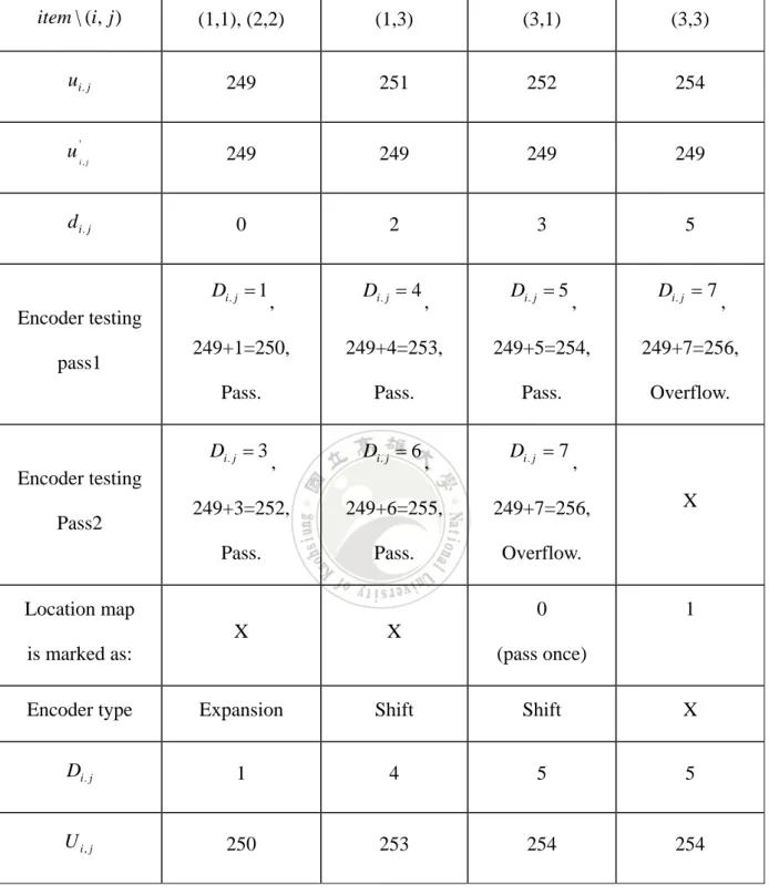
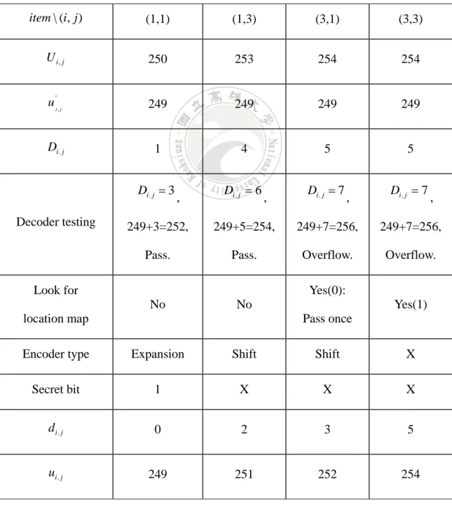
(18) Table 1. The encoder processing step by step.. item \ (i, j ). (1,1), (2,2). (1,3). (3,1). (3,3). ui . j. 249. 251. 252. 254. u 'i , j. 249. 249. 249. 249. d i. j. 0. 2. 3. 5. Di. j  1 Encoder testing pass1. Di. j  4. ,. Di. j  5. ,. Di. j  7. ,. 249+1=250,. 249+4=253,. 249+5=254,. 249+7=256,. Pass.. Pass.. Pass.. Overflow.. Di. j  3 Encoder testing Pass2. ,. ,. Di. j  6. ,. Di. j  7. ,. 249+3=252,. 249+6=255,. 249+7=256,. Pass.. Pass.. Overflow. 0. Location map X. X. 1. X (pass once). is marked as: Encoder type. Expansion. Shift. Shift. X. Di. j. 1. 4. 5. 5. U i, j. 250. 253. 254. 254. 2.5.2 Instance of Decoder Now we can fetch secret bit stream and recover original image by stego image (see Fig. 3) and auxiliary information (e.g. positive threshold P = 1). Table 2. shows the decoder 11.

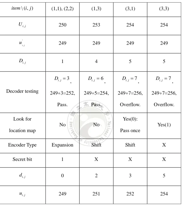
(19) processing step by step. Table 2. The decoder processing step by step.. item \ (i, j ). (1,1), (2,2). (1,3). (3,1). (3,3). U i, j. 250. 253. 254. 254. u 'i , j. 249. 249. 249. 249. Di. j. 1. 4. 5. 5. Di. j  3 Decoder testing. ,. Di. j  6. ,. Di. j  7. ,. Di. j  7. ,. 249+3=252,. 249+5=254,. 249+7=256,. 249+7=256,. Pass.. Pass.. Overflow.. Overflow.. Yes(0):. Look for No. Yes(1). No Pass once. location map Encoder Type. Expansion. Shift. Shift. X. Secret bit. 1. X. X. X. d i. j. 0. 2. 3. 5. ui . j. 249. 251. 252. 254. 12.

(20) 249. v 0 ,1 249. 249. v 0, 0 249. 249. v1, 0. u v1, 2 u v1, 4  1,1  1,3 249 249 249 251 249 v 2 ,1 u 2, 2 v 2,3 249 249  249 249 249 v 3, 0 u v 3, 2 u v 3, 4  3,1  3, 3 249 252 249 254 249 v 4 ,1 v 4,3 249 249 249 249 249 Fig. 4. Distribution of recovery image’s pixel.. 13.

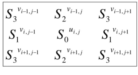
(21) 3. Our method Difference expansion loss its advantages when most predictive differences are not equivalent to zero. This drawback infers not only less capacity, but high distortion. It motivates us to represent our method to avoid this drawback. In our method, we proposed the optimal weight through 3×3 box filter [6] to enhance Sachnev et al.’s prediction [5]. First, we introduce 3×3 box filter, which is used to decrease the noise effect. Second, we present a predictive method, that computes the optional weights to increase the number of zero differences by using the least square technique in linear algebra [11]. And we must correct the definition of local variance in the end. We explain 3×3 box filter, optimal weight and local variance in detail as the following sub-section.. 3.1 3×3 Box Filter As mentioned previously, 3×3 box filter, including cross direction, makes the prediction more accurately in complicated image. We illustrate 3×3 box filter in the following Fig. 5. v. S 2 i1, j u S0 i, j. vi 1, j 1. S2. S 3 i1, j 1 v S1 i , j 1 S3. v. S 3 i1, j 1 v S1 i , j 1. v. vi 1, j. S3. vi 1, j 1. Fig. 5. 3×3 box filter.. All the pixels in the z  z image must be classified into four sets, S0 , S1 , S 2 , S 3 such that. S n   u i , j i % 2   2   j % 2   n  ; 2  i, j  z  1 . The 3×3 box filter cell is. composed. of. original. pixel. value. and. ui, j 14. its. eight. neighbor. pixel-values.

(22) vi 1, j 1 , vi 1, j ,, vi 1, j 1 .. 3.2 The Predictive Method of Optimal Weights Predictive pixel value ui' , j can be written as a linear combination of the eight neighbor pixel-values vi 1, j 1 , vi 1, j ,, vi 1, j 1 : u 'i, j  w1  vi1, j 1  w2  vi1, j  w3  vi1, j 1  w4  vi, j1  w5  vi1, j 1  w6  vi1, j  w7  vi1, j1  w8  vi, j 1 ,. (8). where wk are weights of u 'i , j , for k = 1 to 8. Then, the predictive difference d i , j is computed by d i , j  u i , j  u i' , j .. (9). Our predictive method aims at d i , j  0 by choosing adaptive weights wk .To simplify the representation of symbols, we use the vector ai , j to represent u i , j ’s neighbor pixel-values as:. ai, j＝[vi1, j1 , vi1, j , vi1, j 1 , vi, j1 , vi1, j1 , vi1, j1 , vi1, j , vi1, j 1 , vi, j 1 ] 18 .. (10). And we use the vector x to represent eight weights as:. x＝[w1 , w2 , w3 , w4 , w5 , w6 , w7 , w8 ]T18 .. (11). Then, we rewrite Formula (8) with assuming ui' , j  ui , j for zero difference as: ai , j x  u i , j .. According to the above formula, we get the weight vector x for one cell. 15. (12).

(23) However, the weight vector x should be suitable to neighbor pixel-values for each cell. Obviously, no weight vector x exists such that the predictive difference d i , j  ai , j x  ui , j is zero for each cell. Therefore, we try to search the optimal weight vector x such that the numbers of the zero predictive difference is the most. For. 5102 4. instance,. assume. the. set. has. S0. m. (with. 512 × 512. image,.  65025  m  8 ) cells to be predicted. Let the vector b denote the elements of S0 .. Then, we have. b＝[ui, j , ui, j 2 , ui, j 4 , ui, j6 ,]T1 m . And the matrix A. represents the set of neighbor vector. (13). ai , j according to each cell. as. A＝[ai, j , ai, j 2 , ai, j4 , ai, j8 ,]T8 m .. (14). Here we assume that each cell has the zero predictive difference. Then, we get the following equation as. Ax  b,. (15). from Formula (12). However, linear algebra [11] shows that we can not expect in general to find a vector. x  R 8 for which Ax equals b . Because A is an m  8 ( m >8) matrix, the inconsistent dimensions cause overdetermined system. Instead, we can look for a vector x such that Ax is “closest” to b . Given a system of equations Ax  b , where A is an m  8 matrix and b  R m , then for each x  R 8 we can compute a residual r  x  ,. 16.

(24) r x   b  Ax.. (16). The distance between b and Ax is given by b  Ax  r  x  ,. (17). We wish to find a vector x  R 8 for which r  x  will be minimum. A vector xˆ with the minimum r  x  is said to be a optimal weight to the system Ax  b . The optimal weight xˆ will be a solution to the least square problem Ax  b if and. only if p  Axˆ is the vector in the column space of A ( R( A) ) that is closest to b . The vector p is said to be the projection of b onto R( A) . It follows from Theorem 5.3.1 in linear algebra [12] that b  p  b  Axˆ  r xˆ . (18). must be an element of R( A)  . Thus xˆ is a solution to the least squares problem if and only if r xˆ   R A . . (19). The key to solving the least squares problem is provided by Theorem 5.2.1 [12], which states that.  . R  A   N AT . . (20). A vector xˆ will be a least squares solution to the system Ax  b if and only if r  xˆ   N AT . (21). 0  AT r  xˆ   AT  b  Axˆ .. (22). or, equivalently,. Thus, to solve the least squares problem Ax  b , we must solve the normal equations as 17.

(25) AT Axˆ  AT b.. (23). If A is an m  8 matrix of rank 8, the normal equations have a unique solution xˆ  AT A AT b. 1. (24). and xˆ is the optimal weight to the system xˆ  AT A AT b . 1. We define the predictive pixel values u 'i , j as the element of projection vector p p  [u i' , j , u i' , j  2 , u i' , j  4 , u i' , j 6 ,...] 1Tm .. (25). . (26). The projection vector p  Axˆ  A AT A. . 1. AT b. is the element of R  A that is closest to b in the least squares sense. Now we can realize that the optimal weight xˆ is a least squares solution of m ( number of cells)  8 overdetermined system Ax  b . After obtaining the optimal weight xˆ , we use xˆ to compute predictive pixel value for each cell u i' , j  ai , j xˆ. ui' , j by following formula. (27). Then we can compute predictive difference d i , j by Formula (8). We hope the number of the zero predictive difference d i , j will be the most.. 3.3 Local Variance Because the 3×3 box filter is different with Rhombus Pattern [5], so the local variance.  i, j must be corrected by Formula (28). 18.

(26)  i, j . 1 8 vk  vk 2 ,  8 k 1. (28). Here vk is.  v1  v2  v3 v  4.  v5  vi1, j 1  vi1, j   v6  vi 1, j  vi 1, j 1   v7  vi 1, j 1  vi , j 1 v  v  v i , j 1 i 1, j 1 .  8.  vi 1, j 1  vi 1, j  vi 1, j  vi 1, j 1  vi 1, j 1  vi , j 1  vi , j 1  vi 1, j 1. When the local variance’s value is small, the predictive difference d i , j might be small. Sorting local variance  i, j to determine the computation order of cell d soort makes the stego image maintain low distortion. Next section ,we exploit 3×3 box filter and optimal weight to implement the new algorithm.. 3.4 Algorithm To hide secret bits in cover image, we define the processing order of encoder as S 0 , S1 , S 2 , S 3 . After performing encoder algorithm, we generate a stego image. To fetch secret bits. from the stego image legitimately, we perform decoder algorithm by the processing order: S 3 , S 2 , S1 , S 0 . Once getting secret bits, we can recover the original cover image. Before. describing our algorithm, we give the definition of symbols in our algorithm.. 3.4.1 Definition of Symbols. A. Processing Table Tprocess. T process is constructed by sorting local variance 19.  i, j in ascending order. The first 34.

(27) elements of Tprocess contains the locations of auxiliary information. B. Auxiliary Information. We have to construct the extra 34 bits , auxiliary information, and pass it in the stego image, because decoder need this information. Auxiliary information is composed of 7 bits for positive threshold P , 7 bits for negative threshold N and 14 bits for S k ’s payload size PSk , where 0  k  3 . The auxiliary information provides us to fetch secret bits and to. recover cover image accurately. Insteading of sending the auxiliary. information, we hide. it in the table Tprocess .. C. d sort. According to Tprocess , we compute the predictive differences d i , j of each cell. D. Stream LSB. Stream LSB is composed of LSB of the first 34 elements in d sort . Stream LSB is appended to payload PSk ’s tail as new PSk . We hide Stream LSB for recovering cover image. E. Location Map L. L is used to record the ambiguous result of encoder testing, e.g. ET(b) or ET(c). F. Expandable Set E. E contains cells whose d i , j can be expandable through N and P . G. Shiftable Set S S contains cells whose d i , j can be shiftable through N and P .. 20.

(28) H. Special Set Special. The exception will occur when d i , j belongs to difference expansion and ET(b).. We. should move this cell from E to Special . I. Payload PS0 , PS1 , PS2 , PS3. Secret bits would be parted into 4 uniform sets: PS0 , PS1 , PS2 , PS3 . The set PSi means the payload of. subset S i , for i = 0, 1, 2 and 3.. 3.4.2 Algorithm of Encoder We only introduce encoder algorithm for S0 . For S1 , S 2 and S 3 , we have the similar encoder algorithms. Input: cover image O , payload PS0 (now just secret bits). Output: stego image C , optimal weight xˆ . Step.1). Compute local variance  i , j of each cell in S0 . Construct the processing table Tprocess by sorting  i , j in ascending order.. Step.2). Construct Stream LSB by collecting LSB of ui , j that is located in the first 34 indices of Tprocess . Append Stream LSB to PS0 ’s tail as a new PS0 .. Step.3). Compute optimal weight xˆ according to payload size PS0 and Tprocess .. Step.4). Utilize xˆ to compute predictive value ui' , j , and predictive difference d i , j .. Step.5). Use PS0 and d sort to set threshold P and N . 21.

(29) Step.6). Create a location map L . Set the index k of L to be 0.. Step.7). From the 35th sorted cell in Tprocess , use encoder testing(ET) to check the overflow problem. If check result belongs to ET(a), nothing to do. If check result belongs to ET(b), set L[k ] := 0 and k +1. If check result belongs to ET(c), set L[k ] := 1 and k +1.. Step.8). If the cell belongs to difference expansion method and ET(b), we must move it from E to Special . It means that this cell do not provide a space to hide secret bit.. Step.9). If all cells in S0 are checked such that E < ( L + PS0 ), the gap [ N , P ] must be broadened by 1 ( P := P + 1, N := N - 1).. Step.10) Use Formula (5) to compute modified difference Di , j . If cells belong to E , its d i , j allows to embed secret bit ( PS0 and L ).. Step.11) Compute modified pixel value U i , j by Formula (4) . U i , j substitutes for original pixel value ui , j . Step.12) Auxiliary information substitutes for the LSB of ui , j that is located in the first 34 indices of Tprocess . Step.13) Notice that this stego image C will be input image of the next encoder algorithm for S1 .. 22.

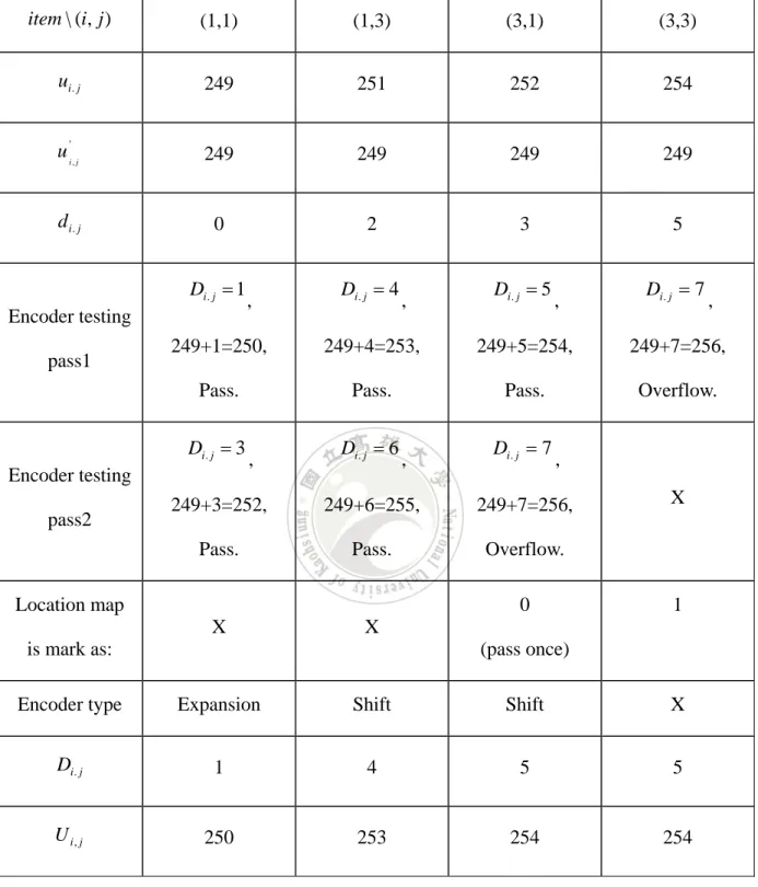
(30) 3.4.3 Instance of Encoder v0 , 0. v0 ,1 249. v1, 0. v0 , 2 249. u1,1. 249 v2,0 249 v3, 0 249 v4,0 249. v0, 0 249. v1, 2. S0 249 249 v 2 ,1 v2, 2 249 249 u 3,1 v3, 2 S0 252 249 v 4 ,1 v4,0 249 249. v0 , 4 249. u1,3. 249 v1, 4. S0 251 249 v2,3 v2, 4 249 249 u 3, 3 v3 , 4 S0 254 249 v4,3 v4, 4 249 249. Fig. 6. Distribution of original image’s pixel.. To realize our algorithm, we give the image in Fig. 6 to explain our algorithm. From Fig. 6, we can obtain the set S0 whose elements are u1,1 , u1,3 , u3,1 and u3,3 . Assume the positive threshold P is 1, test bit is 1 and the secret bit is 1. Assume optimal weight xˆ is computed by pre-processing. We use xˆ to evaluate predictive value u 'i , j for each cell, the assuming result including encoder testing (ET) shows in Table 3. Then we output the stego image (see Fig.7), optimal weight xˆ (pass by another channel) and location map (binary ‘0’ ‘1’). v0 , 0. v0 ,1 249. v1, 0. v0 , 2 249. U 1,1. 249 v2 , 0 249 v3, 0 249 v4 , 0 249. v0 , 0 249. v1, 2. S0 250 249 v2 ,1 v2 , 2 249 249 U 3,1 v3, 2 S0 254 249 v4 ,1 v4 , 0 249 249. v0 , 4 249. U 1,3. 249 v1, 4. S0 253 249 v2 , 4 v2 , 3 249 249 U 3, 3 v3, 4 S0 254 249 v4 , 3 v4 , 4 249 249. Fig. 7. Distribution of stego image’s pixel.. 23.

(31) Table 3. The encoder processing step by step.. item \ (i, j ). (1,1). (1,3). (3,1). (3,3). ui . j. 249. 251. 252. 254. u 'i , j. 249. 249. 249. 249. d i. j. 0. 2. 3. 5. Di. j  1. Encoder testing pass1. Di. j  4. ,. Di. j  5. ,. Di. j  7. ,. 249+1=250,. 249+4=253,. 249+5=254,. 249+7=256,. Pass.. Pass.. Pass.. Overflow.. Di. j  3. Encoder testing pass2. ,. ,. Di. j  6. ,. Di. j  7. ,. 249+3=252,. 249+6=255,. 249+7=256,. Pass.. Pass.. Overflow.. Location map. 0 X. X. 1. X. is mark as:. (pass once). Encoder type. Expansion. Shift. Shift. X. Di. j. 1. 4. 5. 5. U i, j. 250. 253. 254. 254. 24.

(32) 3.4.4 Definition before Decoder Algorithm. A. The Size of Location Map L. After performing decoder testing(DT), we check that cells are ambiguous or not . Move the ambiguous cells from set E or set S to ambiguous set A , and L increase by 1. B. Recovery of Predictive Difference d i , j Di, j / 2, if Di, j [2N;2P 1]  di, j  Di, j  Pp 1, if Di, j  2P 1and P  0 , D  N, if Di, j  2N and N  0  i, j. (29). C. Fetch The Secret Bit b. b  Di, j % 2, if Di, j [2N;2P  1] ,. (30). D. Recovery of Pixel Value ui , j. ui , j  ui, j  di , j ,. (31). 3.4.5 Algorithm of Decoder We only introduce decoder algorithm for S3 . For S 2 , S1 and S0 , we have the similar encoder algorithms. Input: stego image C , optimal weight xˆ . Output: cover image O , payload PS3 (pure secret bits). 25.

(33) Step.1). Compute local variance  i , j of each cell in S3 . Construct the processing table Tprocess by sorting  i , j in ascending order.. Step.2). Reconstruct auxiliary information by fetching LSB of the first 34 U i , j of Tprocess . We discover the secret bits from the first 35th cell in Tprocess .. Step.3). Utilize xˆ to compute predictive value ui' , j and modified difference Di , j .. Step.4). Use auxiliary information to classify cells into expandable set E and shiftable set S.. Step.5). Use decoder testing (DT) to find ambiguous cells (DT(b)). Decoder testing. terminates. Step.6). if E  ( L + PS3 ).. Use Formula (29) to recover unambiguous cells’ predictive difference d i , j . According to d i , j and Formula (30), we can get PS3 and location map L .. Step.7). L is used to recover ambiguous set’s d i , j .. Step.8). Compute original pixel value ui , j by Formula (31), and substitute for the same index’s pixel value.. Step.9). Fetch Stream LSB from the last 34 elements of PS3 . Then Stream LSB substitutes for first 34 U i , j s’ LSB in Tprocess .. Step.10) Output cover image O , PS3 and location map L .. 26.

(34) 3.4.6 Instance of Decoder Now we can fetch secret bit stream and recover original image by stego image (see Fig. 7) and auxiliary information (e.g. positive threshold P = 1, optimal weight xˆ ). We use xˆ to evaluate predictive value u 'i , j for each cell, the assuming result including decoder testing (DT) shows in Table 2. Table 4. The decoder processing step by step.. item \ (i, j ). (1,1). (1,3). (3,1). (3,3). U i, j. 250. 253. 254. 254. u 'i , j. 249. 249. 249. 249. Di. j. 1. 4. 5. 5. Di. j  3. Decoder testing. ,. Di. j  6. ,. Di. j  7. ,. Di. j  7. ,. 249+3=252,. 249+5=254,. 249+7=256,. 249+7=256,. Pass.. Pass.. Overflow.. Overflow.. No. No. Look for. Yes(0):. location map. Yes(1) Pass once. Encoder type. Expansion. Shift. Shift. X. Secret bit. 1. X. X. X. d i. j. 0. 2. 3. 5. ui . j. 249. 251. 252. 254. 27.

(35) Then we output the recovery (see Fig.8) image and secret bit (binary ‘1’). And the instance of our method have completed right now. v0 , 0. v0 , 2. v0 ,1 249. v1, 0. u1,1. 249 v2 , 0 249 v3, 0 249 v4 , 0 249. v0 , 0 249. 249 v1, 2. v0 , 4 249. u1,3. 249 v1, 4. S0 S0 249 249 251 249 v2 , 2 v2 ,3 v2 ,1 v2 , 4 249 249 249 249 u3,1 v3, 2 u3, 3 v3, 4 S0 S0 252 249 254 249 v4 ,1 v4 , 0 v4 , 3 v4 , 4 249 249 249 249. Fig. 8. Distribution of recovery image’s pixel.. 28.

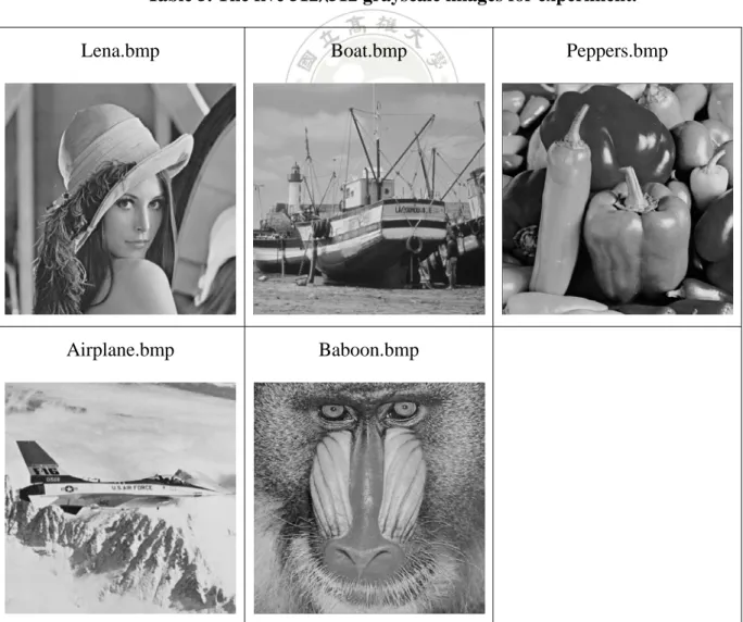
(36) 4. Experiments and Discussion This section compares the experiment results of Sachnev et al.’s method [5], Lin et al.’s method [11] and our method. We choose five images, Lena, Peppers, Baboon, Boat and Airplane, shown as Table 5. The experiment results are shown in Fig. 9 to Fig. 13. The horizontal and vertical axis of the figure denotes payload(bit per pixel) and distortion(Pixel Signal Noise Ratio), respectively. In the same payload condition, the enhanced ratio of average PSNR is shown in Table 6. Table 5. The five 512×512 grayscale images for experiment.. Lena.bmp. Boat.bmp. Airplane.bmp. Baboon.bmp. 29. Peppers.bmp.

(37) Fig. 9. Experiment curve of Lena. Fig. 10. Experiment curve of Peppers 30.

(38) Fig. 11. Experiment curve of Baboon. Fig. 12. Experiment curve of Boat 31.

(39) Fig. 13. Experiment curve of Airplane. Table 6. The enhanced ratio of average PSNR. Compares with. Compares with. Sachnev et al.’s. Lin et al.’s. method [5]. method [11]. Lena. 2.27%. 1.14%. Peppers. 4.10%. 0.11%. Baboon. 9.67%. 1.04%. Boat. 3.31%. 2.17%. Airplane. 1.93%. 1.61%. Our PSNR. method enhanced Ratio. Tested. image. 32.

(40) We can observe the improvement of PSNR at Fig. 3 (Lena) and Table 5. Lena’s row, enhance 1.14% on average. We consider about the worse case(minimum and maximum payload) at Fig. 3, and propose following explanation. In minimum payload, our method embedding 4×34 bit auxiliary information is more than rhombus pattern (2×34 bit). In maximum payload, the embedding order is determine by local variance  i , j , so embedding index do not reuse again. The property leads sparse cell with big difference to be chose, and influence PSNR decrease rapidly. The another advantage of our method is suitable for complex image, like Peppers and Baboon. Our method respectively enhances the PSNR ratio 4.10% with Peppers, 9.67% with Baboon in the condition of same payload. Because optimal weights and 3×3 box filter not only refer to direction of horizontal and vertical, but also refer to direction of skew cross. Optimal weights and 3×3 box filter generate more small difference. Obviously, our method improves the difference expansion.. 33.

(41) 5. Conclusion In this thesis, we use optimal weights and 3×3 box filter to enhance Sachev et al.’s method. In the condition of same payload, experiments show that our method provide better image quality in complex image(5.69%). Optimal weights and 3×3 box filter are efficient to detect noise in surrounding pixel, and compute the appropriate predictive difference for difference expansion method. Generally, the small values of predictive difference generate the stego image with imperceptible changes. Our method can recognize that an accurate prediction contributes obvious performance (such as high capacity, low distortion) to data hiding. Therefore, our method gives the solution of predicting both smooth image and complex image.. 34.

(42) References [1] J. Tian, “Reversible Data Embedding Using A Difference Expansion,” IEEE Trans. Circuits Syst. Video Technol., vol. 13, no. 8, Aug. 2003, pp. 90–896. [2] H. J. Kim, V. Sachnev, Y. Q. Shi, J. Nam, and H. G. Choo, “A Novel Difference Expansion Transform For Reversible Data Embedding,” IEEE Trans. Inform. Forensics Security, vol. 3, no. 3, Sep. 2008, pp. 456–465. [3] A. M. Alattar, “Reversible Watermark Using The Difference Expansion Of A Generalized Integer Transform,” IEEE Trans. Image Processing, vol.13, no. 8, Aug. 2004, pp. 1147–1156. [4] D. M. Thodi and J. J. Rodriguez, “Expansion Embedding Techniques For Feversible Watermarking,” IEEE Trans. Image Procesing., vol. 16, no. 3, Mar. 2007, pp. 721–730. [5] V. Sachnev, H. J. Kim, and J. Nam, S. Suresh, Y. Q. Shi, “Reversible Watermarking Algorithm Using Sorting And Prediction, ” IEEE Trans. Circuits Syst. Video Technol., vol. 19, no. 7, Jul. 2009, pp. 989–999. [6] 林士倫, 鄭宇哲, 陳建源, 施能寅, “九宮格式直方圖的可逆資訊隱藏技術”, TANET 2009 台灣網際網路研討會, 2009, pp.B-94 - B-100. [7] L. Kamstra and H. J. A. M. Heijmans, “Reversible Data Embedding Into Images Using Wavelet Techniques And Sorting,” IEEE Trans. Image Process., vol. 14, no. 12, Dec. 2005, pp. 2082–2090. [8] Z. Ni, Y. Q. Shi, N. Ansari, and W. Su, “Reversible Data Hiding,”IEEE Trans. Circuits Syst. Video Technol., vol. 16, no. 3, pp. 354–362,Mar. 2006. [9] 楊政興, 蔡孟璇, 黃正達, “以棋盤式預測法改善直方圖可逆資訊隱藏技術,” 第十九屆資訊安全會議, 2009. [10] M. U. Celik, G. Sharma, A. M. Tekalp, and E. Saber, “Reversible Data Hiding,” in Proc. Int. Conf. Image Processing, vol. II, Sept. 2002, pp.157–160. [11] 林坪亨, 陳建源, 黃健峯, 林士倫, “基於九宮格式預測法之差值擴張可 35.

(43) 逆資訊隱藏技術,” 2010 資訊安全技術創新應用研討會, 2010, pp.266 – 272. [12] Steven J. Leon, Linear Algebra with Applications, 7th Edition, Pearson Education, Limited, 2006.. 36.

(44)