AN IDENTIFICATION METHOD FOR ESTIMATING THE INERTIA PARAMETERS OF A MANIPULATOR

Institute of Control Engineering National Chiao Tung University Hsinchu 30050, Taiwan, ROC

Received November 29, 1990; accepted June 21, 1991

This article presents an off-line identification method to estimate the minimal knowledge of the inertia parameters for determining the dynamic model of a manipulator. A new approach is proposed to find a set of the minimal knowledge of the inertia parameters. This set is recursively estimated by moving one joint at a time. The off-line identification procedure also provides a sufficient condition for a persistently exciting trajectory. A simulation example of Stanford arm illustrates the validity and simplicity of the identifi- cation procedure.

1. INTRODUCTION

The dynamic system of a manipulator is a nonlinear, coupled multivariable system. Conventionally, each joint of a manipulator is controlled by an inde- pendent PD algorithm.' Because of the nonlinearity and coupling, the propor- tional derivative (PD) algorithm is only justified for some nominal trajectories. On the other hand, the computed torque control uses the inverse dynamics to compensate for the nonlinearity so that the tracking error in the whole work- space can be reduced t o zero.2 Recently, many advanced control for manipulators are all based on the computed torque method. However, good Journal of Robotic Systems 9(4), 505-528 (1992).

506

Journal of Robotic Systems-1 992 performance of these control schemes can be ensured only if the inverse dy- namics of manipulators are known.

Some algorithms based on the efficient recursive Newton-Euler formulation9 satisfied the sampling rate criterion for computing the manipulator inverse dynamics on a multiprocessor systemlo or on a single processor.lI We are then asked if we can get the exact values of the inertia parameters (mass, center of mass, and inertia tensor) required for the recursive Newton-Euler formulation. Armstrong et a1.I2 used a mechanical method to measure the inertia parameters of PUMA 560. Their approach is tedious and requires to disassemble the ma- nipulator. Therefore, a lot of identification methods are proposed for the inertia parameters of manipulators. Atkeson et al.13 showed that the actuator forces of a manipulator are linear functions of the inertia parameters. All works dealing

with the inertia parameter identification tried to or i m p l i ~ i t l y ~ ~ ~ ~ ~ ~ ' formulate the linear equations. Some regrouping rules are also p r e ~ e n t e d ' ~ + ' ~ - ~ ~ to make the number of inertia parameters appearing in the linear equations

minimum since it is found that not all inertia parameters are required to deter- mine the actuator forces. On the other hand, Craig et al.23 developed an identifi- cation algorithm for a parameter-adaptive control scheme.

Among these identification methods, Khosla and KanadeI8 exploited the property that the actuator force of joint i is dependent merely on the inertia parameters of link

i

to link n. They then proposed an off-line identification method by letting only one joint (from joint n to 1) move at a time such that the combinations of the inertia .parameters required in the symbolic dynamic equa- tions are estimated recursively from link n to link l. However, it is cumber- some to form the symbolic dynamic equations and difficult to regroup the terms in the symbolic equations, especially for a robot with six joints.

In this article, we present a new off-line identification method to estimate the inertia parameters for determining the dynamic model of manipulators. A new approach to finding the minimal knowledge of the inertia parameters of a ma- nipulator is proposed, although the result is substantially equivalent to the earlier ones.22,24-28 An identification procedure is then to estimate the minimal knowledge of the inertia parameters. Although the off-line identification method is also to move one joint at a time, only the first rotational joint is required to move in the largest part of the identification procedure. An analytic method is presented to investigate the linear independence of the columns in the linear equations of the dynamic model while only one rotational joint or one translational joint of a manipulator moves. This analysis provides us with the persistently exciting trajectories for identifying the minimal knowledge of the inertia parameters. Another advantage of the present method is that it does not require the symbolic dynamic equations.

The next section introduces the inertia constants of composite bodies, which are found to be able to constitute a set of the minimal knowledge of the inertia parameters for determining the dynamic model of manipulators. In Section 3, we let one rotational joint or one translational joint move alone and relate the actuator forces to the minimal knowledge of the inertia parameters. The analy- sis of these relations allows us to establish an off-line identification procedure.

Definition.

over R"

if

there exist constants ai, i = 1,

.

. .

,

n , not all zero such that

A set of columns a i ( 0 ) : R" + R" is said to be linearly dependent

Zfai are all zero, the set is said to be linearly independent over R".

2. BACKGROUND

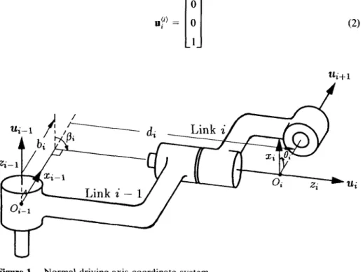
We consider a manipulator with n low-pair joints (i.e., connections with a single degree of freedom), which are labeled as joint 1 to n outward from the base. Assign a body-fixed frame on each joint (i.e., frame Ei is fixed on joint i ) in accord with the normal driving-axis coordinate system."-29 The distance from the origin of Ei to that of Ej is designated as i s , and that to the center of mass of link i as c i .

In the normal driving-axis coordinate system (see Fig. l), the z-axis of a body-fixed frame is the driving axis of the corresponding link, i.e., the unit vector along joint i is

E

"j')=

[8]

f

508 Journal of Robotic Systems-1 992 where superscript (i) denotes the representation of a vector with respect to frame E ; . The distance from the origin of frame E;-l to frame E; is shown to be

where SO; = sin O ; , C8; = cos O i , and b i ,

di,

p i ,

and 8; are the geometrical parameters of the coordinate system and shown in Figure 1. Note, d; = d f

+

q i , 8; = O f ifjoint i is a translational joint; otherwise, d; = dl!, 8; =

el! +

q ; , where q i is the displacement of joint i . That means

df

and 8,: are the null-position values of d; and 8;, respectively. The coordinate transformation matrix from E j - l to Ei is then

CO; -SO;

(4)

O

I

SpiSOi SpiCO;

cpi

CpjSO; CpjCOi -Sp;

The composite body i is defined as the union of link i to link n. Let the mass of the composite body i and the first moment of the composite body about the origin of E; be denoted as m; and

e;,

respectively, which are

m

where mi is the mass of link j . According to Huygeno-Steiner formula,30 the inertia tensor of the composite body i about the origin of frame

Ei

is

where 1)') is the representation of the inertia tensor of link j , about the center of mass, with respect to frame E j , and [ax] denotes a skew-symmetric matrix representing the vector multiplication, i.e., [axlb = a x b. In the context, the overhead symbol A is used to denote the inertia parameters (mass, first moment,

and inertia tensor) of composite bodies. We introduce the following notation

1 for rotational joint i 0 for translational joint i K * = (1 - K i ) =

where hmi is the ( m , i)th entry of the inertia matrix, (.);j denotes the

(i,

j)t h

entry of a matrix, does the x-component of a vector, and

is the acceleration of the origin of frame Ei due to a unit joint acceleration of joint m if joint m is a rotational joint.

The gravitational force of the composite body i is k i g acting at the center of mass of the composite body, where g is the gravitational acceleration. The gravity term of the actuator force (denoted by 7 8 ) applied on joint

i

is to resist

the gravitational forces exerted on joint i by link i along the direction of joint

i,

i.e.

Lemma 1.

be divided into the constant (ki, Ui) and varying

(ti,

Vi) parts as

Thefirst moments and the inertia tensors of composite bodies can

kj

+

t i (12)

51 0

where

Journal of Robotic Systems-1 992

k, = rn,c$)

e,

= 0

v,

= 0 and i f i

<

n

f o r translational joint i

+

1 (i.e., K;+l = 1).

Note that

'+:Rb

is the third column of the coordinate transformation matrix

'+;.R

and

This lemma can be straightforwardly proved by the principle of mathematical induction, for which we refer to Lin.35 For convenience, we name hi, ki and Ui

inertia constants of the composite body i.

Theorem 2. For a manipulator with n low-pairjoints in which joint r is thejirst

rotational joint counting f r o m the base and joint s is the nearest rotational joint not parallel to joint r, a sufficient knowledge of the inertia parameters f o r determining the actuator forces T is the information of the set 9 consisting of

51 2 Journal of Robotic Systems-1 992 4. K;(k;), , K;(ki), , Ki(kJz for s

<

i 5 n

and

where S j = 0 f o r the case that U,//uk//& Vk

<

j

<

s, and i s is zero or parallel to

ur f o r every rotationaljoint m , r 5 m

<

j ; otherwise, Sj = 1; and u; = 0 f o r the

case of ui//ur, r

<

i

<

s ; otherwise ui = 1 .

Proofi We recognize that the dynamic equations of a manipulator with n joints are

H(q, x)q

+

7'(q, q, x)

+

7g(q, x) = 7 (29)

where q E R" consists of the joint displacements, x E R'O" consists of the 10n inertia parameters, 7 E R" consists of the actuator forces, H(q, x) : R"+P +

R""" is the symmetric inertia matrix, 7g(q,

x)

: Rll" + R" consists of the

gravitational forces, T E R" consists of the actuator forces, and F ( q , q, x) : R1*" + R""" consists of the Coriolis, centrifugal forces, which can also be related to the inertia matrix with Christoffel symbols (Cijk)33:

where T ? is the ith element of 7 c , q; is that of q, and hij is the (i, j)th entry of H.

According to (30)-(32), the knowledge of the inertia parameters for determining H is sufficient to determine T ~Thereafter, we just need to investigate the .

inertia parameters in (9) and (1 1).

According to (12), (19), and (23), 4; and then

a!'

can be calculated with the x- and y-components of Kj*kj and Kjmj, j = i

+

1,

.

. .

, n , i.e.

where a i j k , bijk, and Cijk are some appropriate functions.

We can rewrite (25) for translational joint i

+

1 in the form of

where

Equations (21) and (36) reveal that Vi is independent of KjUj, j

>

i, and is a function of Kjmj, Kj$j), the x- and y-components of K:kj and the (3,3)th, (1,2)th, (1,3)th, (2,3)th entries and the difference of the (1,l)th and (2,2)th entries of Kj*Uj, j

>

i.

We examine (9) and (1 1) and find that hrni and T ; are not explicitly related to

the z-component of

t?)

and that only one column, the third column, of KTJy’ is required in calculating the inertia matrix. The observations for (9), ( l l ) , (21), and (36) allow us to conclude that the knowledge of

are sufficient to determine the inertia matrix and gravity load. However, we can still eliminate some elements for link i, i

<

s.

For the case of i

<

r, there are only translationaljoints. Equations (9) and (1 1) are reduced to

51 4 Journal of Robotic Systerns-1992

i

<

r (38)

which implies that Jy) and

g f ) ,

i

<

r, are unnecessary in determining the inertia matrix and the gravity load, nor are U; and kj necessary.

The rotational joints remaining in front of s are parallel to one another. Thus, u:) = [ O , 0, 1IT for rotational joints m and i, r 5 m

<

i

<

s. If joint m is a

rotational joint and joint i is a translational joint, r 5 m

<

i

<

s, u:) = u!) is

constant since the body-fixed frame on a translational joint is invariant to the motion of the nearest rotational joint in front of the translational joint. Equation (9) is then reduced to

T g = -

Equations (1 1) and (39) allow us to delete k, of any rotational joint j , r I j

<

s out of the sufficient knowledge of the inertia parameters if u,//uk//g, V k

<

j

<

s, and i s is zero or parallel to u, for every rotational joint m , r 5 m

<

j. Instead of

k; for translational joint

i,

r

<

i

<

s, a combination of

is sufficient since u;) is constant. Besides, we only need the (3,3)th entry of Jp) for the rotational joints, which contains some Uj and kj, j 2 i.

Suppose that joints i and m , i

<

m 5 s, are rotational joints and joints k,

i

<

m- I

since

implies that the third row of TR is (uj“’) T . (Vi)33 is independent of Urn because

of u:”’ = [0, 0, I I T and it additionally contains the constants

-(u!k’),[(U!k))x(kk)+

+

(~!~’)y(kdyl

+

[I

-

(~!~’)Zl(kk), (43) Note that u,//uj. Therefore, only one entry, the,(3,3)th entry, of K ; U j , r 9 j

<

s, and the combination (43) of the components of kk for translational joint k , r 5 k

<

s, should be included in the sufficient knowledge of the inertia parameters. However, the two combinations (40) and (43) of the components of ki for any translational joint i remaining between joints r and s are unnecessary if the translational joint is parallel to joint r since the x- and y-components of u!’ are

zero in this case. This completes the proof. rn

Remark: In the literature, Gautier et al.22324325 and Mayeda et a1.2c28 investi- gated the minimal knowledge of the inertia parameters for the manipulator dynamic model. The inertia constants listed in Theorem 2 are substantially equivalent to the results of Gautier et al. and Mayeda et al., although some minor terms are different since the set of the minimal knowledge of the inertia parameters is not unique. Another difference is that our approach does not say the inertia constants in Theorem 2 are the minimal knowledge of the inertia parameters for the dynamic model. However, an off-line identification method for estimating these inertia constants will be presented in the next section. Since these inertia constants are all identifiable, they form a set of minimal knowledge of the inertia parameters for determining the dynamic model. The off-line identification method requires an algorithm to compute

ti

and

V i ,

which is proposed as follows.

51 6 Journal

o f

Robotic Systems-1 992 Algorithm 1. To compute

tj

and V j , j 2 r.

Step 1: L e t

4,

= 0 and V,, = 0. I f j = n , g o to step 5 ; otherwise, go to step 2 Step 2: I f joint n is a rotational joint

f o r n - 1 2 s or step 4 for n - 1

<

s.

Otherwise

If

j = n

-

1 , g o to step 5 ; otherwise, let i =: n - 2 and go to step 3

for i 2 s or step 4 for i

<

s.

Step 3: Compute

ti

and

V i

using (19) and (21) ifjoint i

+

1 is a rotational joint. Ifjoint i

+

1 is a translational joint, compute

ti,

i?$+ll) and Vi

Step 4:

Step 5:

using (23), (12), and (36). I f j = i , g o to step 5 ; otherwise, let i =: i -

1 and d o step 3 again for i L s or g o to step 4 for i

<

s.

If

joint i

+

1 is a rotational joint, compute

ti

using (19), otherwise using (23). I f joint i is a rotational joint, in addition compute (Vi)33 using (41). If j = i , g o to step 5 ; otherwise, let i =: i - 1 and do step 4

again.

Vj

and t j , j

<

r , are not required in determining the inertia matrix and the gravity load.

3. OFF-LINE IDENTIFICATION

We intend to identify all the inertia constants listed in Theorem 2 by rotating/ translating one joint at a time. The identification method is backward recursive. The inertia constants

of

the composite body n are first estimated and then used as known values to estimate those of the composite body n

-

1. Finally, all required inertia constants are recursively estimated. The identification proce- dure requires the linear equations. The linear independence of the columns of the matrix in the linear equations implies that the inertia constants in the linear equations are identifiable. In the following, we derive the linear equations for the motion of only one joint and investigate the columns of the matrix in the equations.

Suppose that joints i and j ,

i

<

j , are rotational joints, and joints k , i

<

k

<

j ,

are translational joints. We lock joints j

+

1 to n so that the composite body j

can be seen as a rigid body. Applying Newton-Euler equations, we obtain the inertia force fV and torque tV of the composite body j , acting at the center of mass of the composite body j, as follows

= f < A h ( j ) J J + m(.i) J ( f j j ) m j j ) ) (45)

where

ij

is the inertia tensor of the composite body j about the center of mass of the composite body j , i.e.

and mj and bj are the angular velocity and acceleration of link j , respectively. Let

The dynamic equilibrium states that the force f E j and torque tEj applied by joint

j on link j is in equilibrium with the inertia force and torque and the gravity force of the composite body j , i.e.

51 8 Journal of Robotic Systems-I 992

since

c x [ w x ( 0 x c)] = -(c

-

0 ) ( 0 x c)

+

[c * ( 0 x c ) ] 0

= (0 * c)(c x 0 ) - [ 0

.

(c x 0 ) l c

= - 0 x [c x (c x o)] ₍₅₀₎

3.1. Rotating One Rotational Joint

We rotate joint i but lock all other joints. Under such a condition, the com- posite body k or j can be seen as a rigid body. The actuator force of joint j due to the motion of joint

i

is the component oft$ along the direction of the joint,

i.e.

Similarly, we also get the equation for the actuator force of every trans tionaljoint k, i

<

k

<

j , in the form of

i 1)

a-

( 5 2 )

where qi is the displacement of joint

i.

Substituting (53)-(55) into (51) and (52) yields

r j =

Note that ujk) is invariant since joint k is a translational joint. We are also interested in the actuator force of joint i, which is

since wj‘) =

uj‘)g.

I ? bj‘) =

uj‘)gi

and aj‘) = 0.

The next effort is devoted to examining the linear independence

of

the coeffi- cients on the right sides of (56)-(58). We remark that the x- and y-components of g”’ are linear independent if rotational joints i and j are not parallel to each other since these two components are linearly independent for the case that joint j is not parallel to the gravity direction. If ui is neither parallel nor perpen- dicular to u,, the three components of uij) are nonzero. However, ( ~ j j ) ) ~ = 0 for ui

I

u j , whereas (u(’))~ =

( ~ j j ) ) ~

= 0 for u i / / u j . Thus, we conclude the following.

520 Journal of Robotic Systems-I992

Property 1. Rotating joint i and locking all other joints.

1. Actuator force of rotational joint j , i.e., (56).

(a) The coefficients in (56) are linearly independent over

(4;

, c j i , q j } C R 3 (b) The coefficient of (Uj),, is zero; the other coefficients are linearly (c) Only the coefficient of (Uj)33 is nonzero if u j / / u i / / g and { s / / u ; . (d) Only the coefficients of (UJ)33, (kj), , and (kj),, are nonzero and linearly

if joint j is neither parallel nor perpendicular to joint i.

independent if uj I u;.

independent if uj//ui but uixg or :Sx(Ui.

2 . Actuator force of translational joint k, i.e., (57). (a) kk has no effect on Tk if uk//ui.

(b) The coefficients, q; and

4:,

are linearly independent if ukx(ui. (a) The coefficients in (58) are linearly independent over {q;

,

gi}

C R if 3. Actuator force of rotating joint i, i.e., (58).

u;xg. Otherwise, only the coefficient of (Uj)33 is nonzero.

3.2. Moving One Translational Joint

We now consider another case that all joints except a translational joint k , i

<

k

<

j , are locked. Since only a translational joint is in motion, there is no angular velocity and acceleration. The velocities and accelerations of the links remaining behind joint k are all Ukqk and Ukqk, respectively. Analogous to (51)

and (52), we get the actuator forces of joint j and joint k in the forms of

(60) If joint k is not parallel to joint j , the x- and y-components of up' are linearly independent; otherwise, they are zero.

( k ) ]

rk = &k[qk - (g >z

Property 2. Moving translational joint k and locking all other joints.

1. Actuator forces of rotational joint j , i.e., (59).

(a)

The coefficients in

(59)

are linearly independent over

{ q k

, q j } C R Z if (b) The coefficients in (59) are zero if u j / g and Ujluk.

(a) The coefficient in (60) is nonzero if qk is nonzero. either ujxg or ujXuk.

2. Actuator forces of moving joint k, i.e., (60).

3.3. Off-Line lndentification Procedure

For a rotational joint j , j 2 s, there exists at least one rotational joint, say

joint r, in front of joint j such that joint j is not parallel to it. If the two joints are also not perpendicular to each other, item l(a) in Property 1 implies that there exists a persistently exciting trajectory of qi and q, such that the columns of the matrix in the linear equations formed by (56) are linearly independent. Since

ti

and Vi can be calculated by Algorithm 1 if the inertia constants of links j

+

1 to

n are known, the inertia constants listed in item 2 of Theorem 2 can be esti- mated recursively by using the standard least-squares method.36 If joint j is perpendicular to joint r , we can rotate joint j alone to identify (Uj)33 by using (58), while the other inertia constants are still estimated, according to item I(b) of Property I , in the same way as for the above case.

For a translational joint k, k

>

s, we rewrite (57) in the form of

We denote any two nonparallel rotational joints in front of joint k as joints i and j, i

<

j. There are at least two nonzero components of ujj) for some configura- tions according to (4) and (42). Since ujk) = i R u:” and i R is an orthogonal matrix, there are also at least two nonzero components of uik) for some configu- rations. It is then possible to rotate joint j to find two

or

more configurations in which at least two components of ujk) are nonzero. Under such configurations, the coefficients on the right side of (61) are linearly independent. Therefore, kk for any translational joint k, k

>

s, can be estimated by rotating joint i under at least two such configurations and using (61). This shows that the inertia con- stants listed in item 4 of Theorem 2 are identifiable.

Equation (57) and item 2(b) of Property 1 imply that the inertia constants

listed in item 5 of Theorem 2 are identifiable by rotating joint r.

At last, we consider the rotational joints remaining in front of joint s. In this case, all rotational joints are parallel to one another. However, (Uj>33 for rota- tional joint j , j

<

s, is still identifiable by rotating joint r according to items l(c),

l(d), and 3(a) of Property 1. Item l(d) of Property 1 also indicates that the x-

and y-components of

kj

are identifiable by rotating a rotational joint i, i

<

j , for the case that u,Xg

or

$Xui, whereas item l(a)

of

Property 2 reveals that these components for the case of uj//u,//g//is for any rotational joint i remaining in front of joint j can still be estimated by moving a translational joint k , which remains in front ofjoint j and is not parallel tojoint j , if it exists. This completes

522

Journal of Robotic Systems-1 992

Theorem 4. The inertia constants listed in Theorem 2 are a set of the minimal knowledge of the inertia parameters f o r determining the dynamic model of a manipulator.

Proofi Since the inertia constants in Theorem 2 are all identifiable and are linearly independent, the claim is true.

The proof of Lemma 3 provides us with an off-line identification procedure. Algorithm 2. Off-line identijication procedure.

Step 1: Move one translational joint at a time for every translational joint and use (60) to estimate m k for every translational joint k.

Step 2: Do the following substeps recursively from joint n to joint s . 2.1. For rotational joint j , we compute V j and 4, using Algorithm 1.

Let joint j be neither parallel nor perpendicular to joint r. Under such condition, find three or more configurations of q j such that the components of up) are all nonzero and the first two are not equal. For each of such configurations, we rotate joint Y alone

and measure the values of r j 7

G r ,

and

d r .

These values are substituted into (56) to form the linear equations. Applying the least-squares method, we then estimate [(Uj)l, - (U,)221, ( U ~ ) U ,

If joint j is always perpendicular to joint r , the above method cannot estimate (U,)33. We additionally rotate joint j alone to estimate this value by using (58).

2.2. For translational joint j , we also compute V j and

t j

using Algo- rithm l . We rotate joint s to find two or more configurations such that at least two components of up) are nonzero. For each of such configurations, we rotate joint r alone and measure the values of r j ,

i r ,

and q r . These values are substituted into (61) to form the linear equations. Applying the least-squares method, we then estimate the three components of kj.

Step 3: Do the following substeps recursively from joint s - 1 to joint Y . (Uj>l,, (ujl13 9 (ujl23 9 (kj1.x 9 and ( k j ) y *

3.1. If joint j is a rotational joint, compute (Vj)33 and

( t ) j

using

Algorithm 1.

(a) If u,X(g, we rotate joint r alone and use (56) to estimate (b) If u,/g and there exists a rotational joint i in front of joint j

from which the distance to joint j (i.e., {s) is nonzero and not parallel to joint j , we rotate joint i alone and use (56) again to estimate (Uj),, , (kj)x, and (kj)y.

(c) If u r / g and any rotational joint i in front of joint j satisfies { s / u j , we still rotate joint r and use (56) to estimate (Uj),,

.

However, we check if there is a translational joint

k

in front of joint j that is not parallel to joint j. If there is, we move ( U j h 7 (kj1.x 7 and (kj)y

Mass Center of Mass (m)

(kg) (c:").. (c:")~ (c:")~

9.29 0. 0.1105 0.0175

3.2. Ifjoint j is a translational joint, compute

t j

using Algorithm 1. We rotate joint r alone and apply (57) and the least-squares method to estimate -(utj))z[(u~))x(kj),

+

( ~ ~ ) ) , ( k ~ ) ~ ]

+

[l - (u?)f I(kj)z and -(u?), (kj1.r

+

(uv))x(kj)y.

Inertia Tensor (kg mZ)

(I:i>)i~ (I;<i>)zz (I;<'>)=

0.276 0.255 0.71

The off-line identification procedure is not a unique method. However, it is simple because we rotate joint r alone in the most part of the identification procedure. Since the joint acceleration cannot be very accurately measured in comparison with the joint displacement and velocity, the allowance of one joint in motion at a time in the above procedure can reduce the identification error to some extent. Link (Type) 1 (R) 2 (R) 3 (T) 4 (R) 5 (R) 6 (R) 4. ILLUSTRATIVE EXAMPLE

The Stanford arm has five rotational joints and one translational joint, The normal driving-axis coordinate system16 and the kinematic and dynamic param- eters of the Stanford arm are shown in Figure 2. We assume that the inertia parameters are unknown, and want to use the off-line identification procedure to estimate the minimal knowledge of the inertia parameters.

0 P b d (m) (m) 41 0. 0. 0. qz +90° 90' 0. 0.1529 0. 90" 0. 43 tO.6447 44 0. 0. 0. 45 -90' 90' 0. 0. 4s 90' 0. 0. Y O

::

-0i0541 5.01

1

%_

0.108 0.018 0.1 4.25 -0.6447 2.51 2.51 0.006 1.08 0.0092 0.0054 0.002 0.001 0.001 0.63 -0.0566 0. 0.003 0.003 0.0004 0.51 0. 0. 0.1554 0.013 0.013 0.0003 Figure 2. arm.

524 Journal of Robotic Systems-I 992 The first rotational joint is joint 1, and joint 2 is the nearest rotational joint not parallel to joint 1, i.e., r = 1 and s = 2. Note, joint 1 is parallel to the gravita- tional direction. According to Theorem

2,

the minimal knowledge of inertia parameters is the set of

Although m3 can be estimated individually according to step 1 in Algorithm 2, it can also be identified together with k3 by using step 2.2 in Algorithm 2. For convenience, we skip step 1 of Algorithm 2 and use step 2 to estimate the inertia constants of the composite bodies remaining behind joint 1.

It is easy to find some persistently exciting configurations described in step 2 of Algorithm 2. For example, the following configuration satisfies the require- ment of Algorithm 2

9 = 0.7

where q = [ q l ,

. .

.

, q6IT. The values of u?, j = 2, 3 , 4 , 5, 6, are listed in the

first row of Table I. The other two configurations to form persistently exciting configurations for estimating the inertia constants of composite bodies 2, 4, 5, and 6 are selected the same as (62) except that the corresponding joint displace-

Table I.

three individual exciting configurations. Representations

of uI with respect to the body-fixed frames in

-

-

u(2) .(3) (4) u(’) ( 6 ) I 1 I I 1 1

[

- 0 y ] 0.7648

[

-()0&9]

[

::::a]

2 [ 0 . 7 ]

[

-0.6442 0.

]

[00:);]

[

;:!):;]

[

-0.8624 0.30221

[

0.7648 0.

] [

-0.49271 0.5850 0.6442 0.6442 0.4927 - 0.8624 0.7648 0.7648 0.5850 - 0.8696 - 0.4060 -0.8620

0.7 0.7 0. 0.7 0.7 0.7

. .

0.7 0.7 0. 0.7 0.7 -0.6

. .

, q = 0.7 0.7 0. 0.7 0.7 -0.7 ,

-Another configuration for estimating the inertia constants of composite body 3 is that the displacement of joint 2 is changed to -0.7 while the other joint displacements are kept the same as (62). The values of up) for the second and third configurations of the individual identification process are also listed in Table I.

Under each of the above configurations, we rotate joint 1 from the displace- ment of 0.7 to 1.223 rad (i.e., a rotation of 30"). We assume there is a controller installed in the power driver of the actuator on joint 1 such that the response of the joint angle to a step input is a second-order critically damping with damping time constant l/cr = 1/1Os, i.e.

We arbitrarily select three sets of the values of T ~ , q l , and q I , say at r = 0 . 2 , 0 . 3 , and 0.4, and substitute them into (56) and (57) to form the linear equations. Using a package of the least-squares method, we then estimate the inertia constants of composite bodies 2, 3, 4, 5, and 6. Since joint 2 is perpendicular to joint 1, (U2)33 is not yet identified. We rotate joint 2 alone, take one set of the

values of T~ and

&,

and use (58) to estimate (U2)33. (u1)33 is also estimated in the

same manner. The identified values of the minimal knowledge of the inertia parameters of the Stanford arm are shown in Table 11.

It should be remarked that the example is performed in a computer simula- tion. The actuator forces are calculated by a software of the recursive Newton- Euler formulation when the joint displacements, velocities, and accelerations are given. We also write a program, which uses the identified values of the minimal knowledge of the inertia parameters and sets the inertia constants of

526

Journal of Robotic Systems-1 992 Table 11.

Composite

Identified values of inertia constants of the composite bodies.

Body i 1 2 3 4 5 6 -0.oooO1 0.0099 ki -

[

2.7400

]

[

8:

]

[ o . o y ]

-2.7400 (u;)ll-(u;)22 - 4.3850 - -0.0235 - 0.00003 - - 0 .00005 - -0.00003 - 1.0144 4.4053 - 0.0044 (Ui133 (Ui112 (ui)l3 (ui)23 0. 0. - 0. - [-o!i49]

E]

0.0270 0. 0.0277 0.0003 0. 0. 0. 0. 0. 0.

composite bodies other than those in Theorem 2 to zero, to compute the inertia matrix and the gravity load by using (9) and (11)-(13). We find the results are the same as those using another method presented in Lin.32 This verifies our theorems and the off-line identification procedure.

5. CONCLUSION

We have presented a new approach to finding a set of the minimal knowledge of the inertia parameters for determining the manipulator dynamics. An identifi- cation procedure is only to estimate the inertia constants in the minimal knowl- edge of the inertia parameters. The central topic of this article is then to de- velop such an off-line identification method. The identification procedure demands only to move one joint (the first rotational joint in the most part of the procedure) at a time for recursively estimating the minimal knowledge of the inertia parameters. A simulation example of the Stanford arm verifies the off- line identification procedure. The main advantage of our method is that the identification procedure does not require the symbolic dynamic equations.

Finding a persistently exciting trajectory is always a difficult problem in the identification. A r m ~ t r o n g ~ ~ addressed a method of generating the optimal iden- tification trajectory, whereas trial and error methods are widely used in the literature. 1 3 3 1 5 , 1 7 On the contrary, our off-line identification procedure provides

a sufficient condition for a persistently exciting trajectory and allows the identi- fication method to be easily implemented.

This article was supported by the National Science Council, Taiwan, under Grant No. NSC80-0404-E-009-3 1.

References 1.

2.

J. Y. S. Luh, “Conventional controller design for industrial robots-a tutorial,” IEEE Trans. Systems, Men, Cybern., SMC-13, 298-316 (1983).

B . R. Markiewicz, “Analysis of the computed torque drive method and compari- son with conventional position servo for a computed-controller manipulator,” Tech. Memo. 33-601, Jet Propulsion Lab., Pasadena, CA, 1973.

4. 5. 6. 7. 8. 9. 10. 1 1 . 12. 13. 14. 15. 16. 17. 18. 19. 20. 21. 22. 23. 24.

E. G. Gilbert and I. J. Ha, “An approach to nonlinear feedback control with applications to robotics,” IEEE Trans. Systems, Man, Cybern., SMC-14,879-884 ( 1984).

S. K. Lin, “Simulation study of PD robot Cartesian control,” Proc. of 1989 IEEE

Int. Conf. on Robotics and Automation, 1989, pp. 1221-1226.

G. L. Luo and G. N. Saridis, “L-Q design of PID controllers for robot arms,” M. W. Spong and M. Vidyasagar, “Robust linear compensator design for nonlin- ear robotic control,” IEEE J . Robo. Auto., RA-3, 345-351 (1987).

C. W. Wampler and L. J. Leifer, “Applications of damped least-squares methods to resolved-rate and resolved-acceleration control of manipulators,” Trans.

ASME J . Dynamic Systems, Meas., Control, 110, 31-38 (1988).

J. Y. S. Luh, M. W. Walker, and R. P. Paul, “Online computational scheme for mechanical manipulators,” Trans. ASME J . Dynamic Systems, Meas., Control,

H. Kasahara and S. Narita, “Parallel processing of robot-arm control computation on a multi-microprocessor system,” IEEE J . Robo. Auto., RA-1, 104-113 (1985).

S. K . Lin, “Microprocessor implementation of the inverse dynamic system for industrial robot control,” Proc. of 10th IFAC World Congress on Automatic Con-

trol, Munich, FRG, July 27-31, 1987, pp. 332-339.

B. Armstrong, 0. Khatib, and J. Burdick, “The explicit dynamic model and iner- tial parameters of the PUMA 560 arm,” Proc. of I986 1EEE Conf. on Robotics and

Automation, San Francisco, CA, 1986, pp. 510-518.

C. G. Atkeson, C. H. An, and J . M. Hollerbach, “Estimation of inertial parame- ters of manipulator loads and links,” I n f . J . Robo. Res. 5(3), 101-119 (1986). M. Gautier, “Identification of robot dynamics,” Proc. of IFAC Symp. on Theory of Robotics, Vienne, 1986, pp. 351-356.

M. Gautier and W. Khalil, “On the identification of the inertial parameters of robots,” Proc. of 1988 IEEE Conf. on Decision and Control, 1988, pp. 2264-2269. M. Gautier and W. Khalil, “Identification of the minimum inertial parameters of robots,” Proc. of 1989 IEEE Conf. on Robotics and Automation, 1989, pp. 1529- IEEE J . Robo. Auto., RA-1, 152-159 (1985).

102, 69-76 (1980).

1534.

I. J. Ha, M. S. KO, and S. K. Kwon, “An efficient estimation algorithm for the model parameters of robotic manipulators,” IEEE Trans. Robo. Auto., 5, 386-394 (1989).

P. K. Khosla and T. Kanade, “Parameter identification o f robot dynamics,” Proc. of IEEE Conf. on Decision and Control, 1985, p p . 1754-1760.

A. Mukerjee and D. H. Ballard, “Self-calibration in robot manipulations,” Proc.

of 1985 lEEE Conf. on Robotics and Automation, 1985, pp. 1050-1057.

H. B. Olsen and G. A. Bekey, “Identification of parameters in models of robots with rotary joints,” Proc. of 1985 IEEE Conf. on Robotics and Automation, 1985,

pp. 1045-1049.

H. B. Olsen and G. A. Bekey, “Identification of robot dynamics,” Proc. of 1986

IEEE Conf. on Robotics and Automation, San Francisco, CA, 1986, pp. 1004- 1010.

M. Gautier and W. Khalil, “A direct determination of minimum inertial parame- ters of robots,” Proc. of 1988 IEEE Conf. on Robotics and Automation, 1988, p p . J . J . Craig, P. Hsu, and S. S. Sastry, “Adaptive control of mechanical manipula- tors,” Int. J . Robo. Res., 6(2), 16-28 (1986).

M. Gautier and W. Khalil, “Direct calculation of minimum set of inertial parame- ters of serial robots,” IEEE Trans. Robo. Auto., 6, 368-373 (1990).

528

Journal of Robotic Systems-I 992 25. 26. 27. 28. 29. 30. 31. 32. 33. 34. 35. 36. 37.

M. Gautier, F. Bennis, and W. Khalil, “The use of generalized links to determine the minimum inertial parameters of robots,” J. Robo. Systems, 7,225-242 (1990). H. Mayeda, K. Yoshida, and K. Osuka, “Base parameters of manipulator dy- namics models,” Proc. of 1988ZEEE Conf. on Robotics andAutomation, 1988, pp. 1367-1372.

H. Mayeda, K . Yoshida, and K. Osuka, “Base parameters of dynamics models for manipulators with rotational and translational joints,” Proc. of 1989 ZEEE Conf. on Robotics and Automation, 1989, pp. 1523-1528.

H. Mayeda, K. Yoshida, and K. Osuka, “Base parameters of manipulator dy- namics models,” ZEEE Trans. Robo. Auto., 6 , 312-321 (1990).

J. J. Craig, Introduction to Robotics: Manipulation and control. Addison-Wesley, Reading, MA, 1986.

J. Wittenburg, Dynamics of Systems of Rigid Bodies, B. G. Teubner, Stuttgart, 1977, p. 36.

J. W. Burdick, “An algorithm for generation of efficient manipulator dynamic equations,” Proc. of 1986 ZEEE Znt. Conf. on Robotics and Automation, San Francisco, CA, 1986, pp. 212-218.

S. K. Lin, “A new composite body method for manipulator dynamics,” J . Robo. Systems, 8, 197-219 (1991).

N. Renaud, “An efficient iterative analytical procedure for obtaining a robot ma- nipulator dynamic model,” in Robotics Research, M. Brady and R. Paul, Eds., MIT Press, Cambridge, MA, 1984, pp, 749-764.

N. Renaud, “A near minimum iterative analytical procedure for obtaining a robot manipulator dynamic model,” in Dynamics of Multibody Systems, G. Bianchi and W. Schiehlen, Eds., Springer-Verlag, Berlin, 1986, pp. 201-212.

S. K. Lin, “Identification of the inertia parameters of an industrial robot,” NSC Project Report NSC80-0404-E-009-3 1 , 1991.

C. H. Lawson and R. J. Hanson, Solving Least Squares Problems, Prentice Hall, Englewood Cliffs, NJ, 1974.

B. Armstrong, “On finding exciting trajectories for identification experiments in- volving systems with nonlinear dynamics,” Znt. J. Robo. Res., 8(6), 28-48 (1989).