信賴區間與模擬研究-對於穩定表現型的遺傳解釋比例

國

立

交

通

大

學

統計學研究所

碩

士

論

文

信賴區間與模擬研究

-對於穩定表現型的遺傳解釋比例

Confidence Interval and Simulation Studies for

the Proportion of Heritability Explained by

Endophenotypes

研 究 生：謝志強

指導教授：黃冠華 博士

信賴區間與模擬研究

-對於穩定表現型的遺傳解釋比例

Confidence Interval and Simulation Studies for the Proportion of

Heritability Explained by Endophenotypes

研 究 生：謝志強 Student :

Chin-Chiang Hsieh

指導教授：黃冠華 Advisor :

Dr. Guan-Hua Huang

國 立 交 通 大 學

統計學研究所

碩 士 論 文

A Thesis

Submitted to Institute of Statistics

College of Science

Nation Chiao-Tung University

in partial Fulfillment of the Requirements

for the degree of Master

in

Statistics

June 2006

Hsinchu, Taiwan, Republic of China

信賴區間與模擬研究

-對於穩定表現型的遺傳解釋比例

學生 : 謝志強 指導教授 : 黃冠華博士

國立交通大學統計學研究所

摘 要

在生物學上，穩定表現型(endophenotype)和疾病有著相同的

遺傳路徑，但穩定表現型卻比診斷上的表現型(phenotype)更為接

近其相關的基因，這也顯示穩定表現型在複雜疾病上基因研究的

重要性，在這篇報告裡，針對一個由穩定表現型所發展的指標，

即穩定表現型的遺傳解釋比例，我們透過模擬提供其相關意義，

同時，我們也提供此指標的信賴區間，藉此執行統計檢定和統計

推論，除外，透過信賴區間和模擬的結果，建構一些準則，以幫

助我們找尋有用的穩定表現型。

關鍵字：穩定表現型；遺傳率；基因分析

Confidence Interval and Simulation Studies for the Proportion of

Heritability Explained by Endophenotypes

Student :

Chin-Chiang Hsieh

Advisor :

Dr.Guan-Hua Huang

Institute of Statistics

National Chiao Tung University

Abstract

Endophenotypes, which involve the same biological pathways as

diseases but presumably are closer to the relevant gene action than

diagnostic phenotypes, have emerged as an important concept in the

genetic studies of complex diseases. In this report, we give some

patterns about the developed index, the proportion of heritability

e x p l a i n e d ( P H E ) b y t h e e n d o p h e n o t y p e s f o r v a l id a t i n g

endophenotypes. Besides, we provide a relevant confidence interval

of PHE to perform a statistical test and to make some statistical

inference. Using the relevant confidence interval of PHE, we

construct some criteria to help us search a useful endophenotype.

誌 謝

CONTENTS

ABSTRACT(in Chinese) i

ABSTRACT(in English) ii

ACKNOWLEDGEMENTS(in

Chinese)

iii

CONTENTS

iv

LIST OF TABLES

v

LIST OF FIGURES vi

1 Introduction………1

2 Literature review………3

2.1 Statistical validation of surrogate endpoints………..3

2.2 Statistical framework in genetic epidemiology………..4

3 Method………9

3.1 Model……….9

3.2 Estimation……….13

3.3 Hypothesis Test………19

4 Simulation studies….………19

4.1 Study design……….19

4.2 Result………22

4.2.1 PHE……….22

4.2.2 The accuracy of the estimators of the standard error of

PHE……….23

4.2.3 Test of PHE………24

5 Discussion……….27

Appendix………30

Reference………34

LIST OF TABLES

Table 1.Genetic components of variance assuming mating……….. 8

Table 2.The covariance compnonts for relative pairs…………...15

Table 3.The derivative of covariance compnonts for relative pairs..17

Table 4.Parameter setting under scenario II (1)………21

Table 5.Parameter setting under scenario II (2)………21

Table 6.Simulation results based on scenario I (1)………...37

Table 7.Simulation results based on scenario I (2)………...38

Table 8.Simulation results based on scenario I (3)………...39

Table 9.Simulation results based on scenario I (4)………...40

Table 10.Simulation results based on scenario II with P>E (1)……41

Table 11.Simulation results based on scenario II with P>E (2)……42

Table 12.Simulation results based on scenario II with P>E (3)……43

Table 13.Simulation results based on scenario II with P>E (4)……44

Table 14.Simulation results based on scenario II with P<E (1)……45

Table 15.Simulation results based on scenario II with P<E (2)……46

Table 16.Simulation results based on scenario II with P<E (3)……47

LIST OF FIGURES

Figure 1.A surrogate endpoint versus an endophenotype in the disease

process………..49

Figure 2.Two scenarios verified in the simulation studies………….50

Figure 3.Scenario I histogram with family 200………..51

Figure 4.Scenario I histogram with family 500……….……….52

Figure 5.Scenario I histogram with family 200 & ρ

=0.5…………..53

Figure 6.Scenario I histogram with family 500 & ρ

=0.5…………..54

Figure 7.Scenario II histogram with family 200 & P>E …..……….55

Figure 8.Scenario II histogram with family 500 & P>E …..……….56

Figure 9.Scenario II histogram with family 200 & P>E & ρ

=0.5…57

Figure 10.Scenario II histogram with family 500 & P>E & ρ

=0.5..58

Figure 11.Scenario II histogram with family 200 & P<E ………….59

Figure 12.Scenario II histogram with family 500 & P<E ………….60

Figure 13.Scenario II histogram with family 200 & P<E & ρ

=0.5...61

Figure 14.Scenario II histogram with family 500 & P<E & ρ

=0.5...62

Figure 15.Scenario I mean LOD-score curve with family 200……..63

Figure 16.Scenario I mean LOD-score curve with family 500……..64

Figure 17.Scenario I mean LOD-score curve with family 200 &

Figure 18.Scenario I mean LOD-score curve with family 500 &

ρ

=0.5……….66

Figure 19.Scenario I mean LOD-score curve with family 200 &

P>E………..67

Figure 20.Scenario I mean LOD-score curve with family 500 &

P>E……….68

Figure 21.Scenario I mean LOD-score curve with family 200 &

P>E & ρ

=0.5.……….69

Figure 22.Scenario I mean LOD-score curve with family 500 &

P>E & ρ

=0.5 .………70

Figure 23.Scenario I mean LOD-score curve with family 200 &

P<E……….71

Figure 24.Scenario I mean LOD-score curve with family 500 &

P<E……….72

Figure 25.Scenario I mean LOD-score curve with family 200 &

P<E & ρ

=0.5.……….73

Figure 26.Scenario I mean LOD-score curve with family 500 &

P<E & ρ

=0.5.………74

1

INTRODUCTION

In diseases with classic or Mendelian genetics as their distal causes, genotypes are usually indicative of phenotypes. However, this degree of genetic certainty does not exist for complex disease [Gottesman and Gould, 2003]. These “complex” diseases are influenced by multiple genes, environmental factors and their interactions on phenotypes. It leads the direct relation-ship between phenotype and genotype disrupted because that the same genotype may give rise to different phenotypes or the same phenotype may have arisen from different genotypes. To facilitate the identification of influential genetic markers of complex diseases, the endopheno-type approach has been advocated. Other synonymies of endophenoendopheno-type, such as intermediate phenotype, biological marker, sub-clinical trait, vulnerability marker, and phenotypic uncer-tainty, have been used interchangeably with slightly different implications. Gottesman and Gould [2003] provided a means of endophenotyps for identifying the “downstream” traits or facets of clinical phenotypes, as well as the “upstream” consequences of genes, and suggested the following five useful criteria for identification of endophenotypes:

1. The endophenotype is associated with illness in the population. 2. The endophenotype is heritable.

3. The endophenotype is primarily state-independent (manifests in an individual whether or not illness is active).

4. Within families, endophenotype and illness co-segregate.

5. The endophenotype found in affected family members is found in non-affected family members at a higher rate than in the general population.

Hence, the endophenotype is closer to the underlying gene than the phenotype in the course of disease’s natural history. Endophenotype-based genetic analysis is more likely to succeed than phenotype-based one in terms of search for the susceptibility genes; nevertheless, there are emerging needs of systematic statistical methods for endophenotype-based analysis.

On the other hand, surrogate endpoints have been frequently utilized in clinical research, especially in chronic diseases, when the primary endpoint is costly or time-consuming to obtain. A good deal of statistical research in the evaluation of surrogate endpoints have been undertaken for decades. Prentice [1989] presented a landmark definition of surrogate endpoints. Freedman et al. [1992] introduced “the proportion of treatment effect on the primary endpoint explained”(P T E) by the surrogate to supplement Prentice’s criteria.

Conceptually, an endophenotypes is a “downstream” biomarker for detection of heritable biological underpinning and a surrogate endpoint is an “upstream” biomarker for evaluation of treatment effect as illustrated in Figure 1. Noticeably, the causal pathway of intervention-surrogate endpoint-primary endpoint in intervention-surrogate analysis can be seen as an analogy of the pathway of genotype-endophenotype-phenotype in endophenotypes-based analysis. Both en-dophenotypes and surrogate endpoints lie in a biological pathway, but with two important differences: (i) the endophenotype is expected to be closer to the upstream genotype to in-crease the chance of identifying it, though the surrogate endpoint intends to substitute the downstream primary endpoint, and (ii) when the purpose of the study is to identify responsi-ble genes for the phenotype, genotype information is usually unknown, whereas treatment in validating a surrogate is known.

Huang et al. [2005] defined an endophenotype to be “a trait for which a test of null hypothesis of no genetic heritability implies the corresponding null hypothesis based on the phenotype of interest” and developed a formal statistical methodology for accessing the util-ity of endophenotypes, motivated by the conditioning strategy used for surrogate endpoints commonly seen in clinical research. The methodology is especially useful for the situation where underlying genotype is unknown in that researchers use endophenotypes to increase opportunities of finding susceptible disease genes, not to verify whether a specific gene is the cause of disease. Similar to validating surrogate endpoints, various indices can be provided to use to validate endophenotypes. One of the indices is the proportion of heritability explained (P HE) by the endophenotype, similar to P T E introduced by Freedman et al. [1992].

Several authors had pointed out the major difficulty of using P T E: the confidence interval of P T E is generally too wide to convey any useful information. That is, the true P T E might

be anywhere from zero to well over 100% or be negative. To avoid the confidence interval of P HE far too wide to be of practical relevance, we provided a relevant confidence interval of P HE. Futhermore, for P HE, we perform a statistical test or to establish some criteria for determining whether there is an endophenotye. Also, extensive simulation studies were performed to verify the usefulness of P HE.

2

LITERATURE REVIEW

2.1

In most clinical researches, the primary endpoint is too difficult or costly or time-consuming to obtain, particularly in chronic diseases. It may force the investigators to use a substitute or “surrogate”, instead of true endpoint. Surrogate endpoints have been of clinical interest for decades, but it was not until Prentice published a seminal paper in 1989 that formal statistical investigation started. Prentice defined a surrogate endpoint to be “a response variable for which a test of null hypothesis of no relationship to the treatment groups under comparison is also a valid test of the corresponding null hypothesis based on the true (clinical) endpoint”. Prentice’s definition can be written as

f (S _{| X) = f (S) ⇐⇒ f (T | X) = f (T )} (1)

where T denotes the status of a primary endpoint, S denotes the status of a surrogate end-point, X is the treatment variable, f(S) is the distribution of S, and f(S|X) is the conditional distribution of S given X. Validation of Prentice’s definition involves the following two criteria:

f (T _{| S) 6= f (T ) and f (T | S, X) = f (T | S)} (2)

[Prentice, 1989; Freedman et al., 1992; Buyse and Molenberghs, 1998]. The first criterion states that the surrogate endpoint must be correlated with the primary clinical endpoint, and the second criterion is that the surrogate endpoint should fully capture the treatment effect on the primary endpoint.

The surrogate endpoint described by Prentice mediates all of the effect of treatment on the primary endpoint, that is

X _{→ S → T}

A more complex, but more likely, situation arises when treatment has a direct effect on the primary endpoint that is not mediated through the surrogate [De Gruttola et al., 2001]:

X _{→ S → T}

Freedman et al.[1992] proposed to focus on the proportion of the treatment effect mediated through the surrogate. A good surrogate is one that explains a large proportion of that effect. The proposal can be made in the content of generalized linear models [McCullagh et al., 1989]. The net effect of X on T can be assessed through the regression coefficient β_T in the generalized linear model

g [E (T )] = αT + βTX (3)

where g (•) is the link function connecting the mean response and covariates, and the effect of X on T after inclusion of S is the regression coefficient βT S in the following generalized linear model

g [E (T )] = αT S+ βT SX + γT SS (4)

The proportion of the treatment effect (on the primary endpoint) explained (P T E) by the surrogate is given by

P T E = 1₋βT S

β_T (5)

The 100 (1 − α) % confidence limits of P T E can be calculated using Fieller’s theorem or the delta method [Buyse and Molenberghs, 1998]. Using Fieller’s theorem is generally preferable the 100 (1 − α) % confidence limits of PTE [Herson, 1975].

2.2

First, consider a genetic locus defined by two alleles. If we assume two allelic variants, Q and q with frequencies of pQ and (1 − pQ) at a given quantitative-trait locus(QT L), the

genotype-specific means are given by μQQ= μ+a, μQq = μ+d, and μqq = μ−a. The genotypic mean values can be reparameterized in terms of μ0

QQ = a, μ0Qq = d, and μ0qq = −a, so that the mean, μ0_{, is p}2

Qa + 2pQ(1− pQ) d + (1− pQ)2(−a) and the variance about the mean, σ2g, is p2 Q ¡ μ0 QQ− μ0 ¢2 + 2pQ(1− pQ) ¡ μ0 Qq− μ0 ¢2 +(1 − pQ)2 ¡ μ0 qq− μ0 ¢2

. The variance about mean can be decomposed as σ2_g = σ2_a+ σ2_d (6) where σ2_a = 2pQ(1− pQ) £ pQμ0QQ+ (1− 2pQ) μ0Qq− (1 − pQ) μ0qq ¤2 (7) = 2pQ(1− pQ) [a + d (1− 2pQ)] 2

is called the additive component of variance, and

σ2_d = ©pQ(1− pQ) £

μ0_{QQ− 2μ}0_Qq+ μ0_qq¤ª2 (8)

= [2pQ(1− pQ) d]

is called the dominance component of variance [Duggirala et al., 1997].

Let Gi and Gj represent the genotype of two individuals i and j. In general, under Hardy-Weinberg equilibrium and no inbreeding, the genetic covariance can be expressed as

cov (Gi, Gj) = 2φijσ2a+ ∆ijσ2d (9)

where, φ_ij , the coefficient of kinship ,or coefficient of coancestry, is defined as the probability of randomly drawing a single allele in individual i that is identical by decent (ibd) to a single allele at the same locus randomly drawn from individual j, and ∆ij , the fraternity coefficient, is defined as the probability that both alleles at a locus are shared ibd by individuals i and j [Duggirala et al.,1997].

After all, it is not very realistic. The involvement of several loci in the determination of the trait may be considered. Assume that there are m QT Ls to influence the actual trait. If

the effects of single loci are independent, the covariance can be written as

cov (Xi, Xj) = 2φijσ 2

A+ ∆ijσ2D (10)

where Xi and Xj represent, respectively, the actual trait of individuals i and j, σ2A=

Pm

k=1σ 2 ak is the total additive genetic variance, σ2D =

Pm

k=1σ 2

dk is the total dominance genetic variance and σ2

ak and σ2dk , are the additive and dominance genetic variance due to the kth locus, respectively [Iachine, 2004].

Besides, to describe the residual variation of the trait when the genotype is fixed, the so-called environmental effects may be introduced. Suppose the effects of genes and environment are additive. Under the additional assumption of independence between genotypic effects and environmental effects, the covariance can be written as

cov (Xi, Xj) = 2φijσ 2

A+ ∆ijσ2D+ V ar (XE,ij) (11)

where XE,ij is environmental effect between individual i and individual j [Iachine, 2004]. In particular, this implies the following structure of the trait variance:

V ar (Xi) = σ2A+ σ 2

D+ V ar (XE,i) (12)

where XE,i is environmental effect of individual i. If we further assume, that we have the same the environmental variance V ar (XE) and total variance σ2 for all family members, the structure of the trait variance can be written as

σ2 = σ2_A+ σ2_D+ V ar (XE) (13)

A study point for many scientists investigating disease aetiology has often been to study the heritability of a particular trait. Formally, the heritability of a continuous trait is defined as the proportion of its total variance (σ2_{) that is attributable to genetic factors in a} particu-lar population. Narrow-sense heritability is defined as σ2

(σ2A+ σ2D) /σ2. Usually, it is of interest to know the broad-sense heritability because its value can be used to predict the effect of searching for genes [Iachine, 2004; Burton and Tobin, 2003]. Let us decompose V ar (XE) into σ2C and σ2E ,where σ2C is called the shared environ-mental component of variance and σ2

E is called the non-shared environmental component of variance,i.e.

σ2 = σ2_A+ σ2_D+ σ2_C+ σ2_E (14)

In some practical problems, it is often assumed that the dominance component of variance is negligible(i.e. σ2D = 0), leading to the so-called ACE model.

As in mainstream epidemiology, many of the relevant models may helpfully be viewed as being generalized linear mixed models [Breslow and Clayton, 1993.]. Here,we will consider the structure of one such GLMM.

A general model with wide applicability may be written as

g¡μij ¢ = ηij = α + β T zij + ξij, (15) Yij ∼ f ¡ μ_ij, ¢ ξ_{ij ∼ N}¡0,£σ2_A+ σ2_D+ σ2_C¤¢ cov¡ξij, ξik ¢

[j _{6= k] = 2φ}ij,ikσ2A+ ∆ij,ikσ2D+ λij,ikσ2C

where Yij is the observed phenotype in the jth member of the ith family, μij is the its expected value, and f (•) denotes an error distribution which may incorporate a nuisance parameter denoted [Burton and Tobin, 2003]. The expected value of the phenotype is predicted via a link function g (•) applied to a linear predictor ¡ηij

¢

comprising a baseline mean (α), a vector of observed covariates (zij), a corresponding vector of unknown regression parameters (β) and subject-specific random effects ξij with an appropriate covariance structure. The components σ2

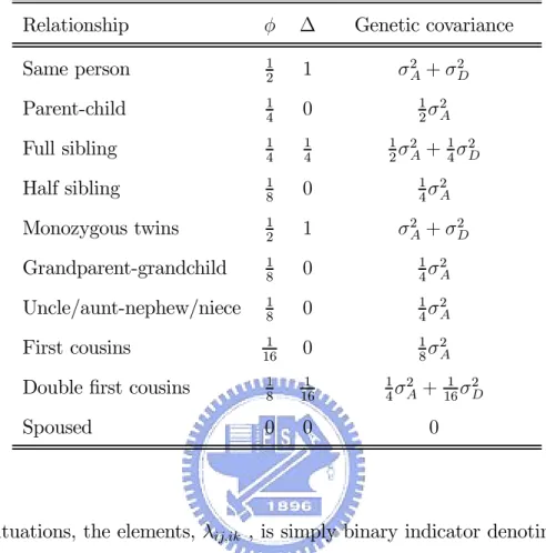
A, σ2D and σ2C represent, respectively, the variances arising from polygenic additive effects, polygenic dominance effects and shared environmental effects [Hopper, 2002]. The terms φ_ij,ik and ∆ij,ik denotes, respectively, the kinship coefficient and fraternity coefficient between individuals ij and ik. Table 1 details the φij,ik and ∆ij,ik values for selected relative pairs and

the total genetic variances that these imply [Burton and Tobin, 2003].

Table 1. Genetic components of variance assuming mating

Relationship φ ∆ Genetic covariance

Same person 1 2 1 σ 2 A+ σ2D Parent-child 1₄ 0 1₂σ2 A Full sibling 1₄ 1₄ 1₂σ2 A+ 1 4σ 2 D Half sibling 1₈ 0 1₄σ2 A Monozygous twins 1₂ 1 σ2 A+ σ2D Grandparent-grandchild 1₈ 0 1₄σ2A Uncle/aunt-nephew/niece 1 8 0 1 4σ 2 A First cousins 1 16 0 1 8σ 2 A

Double first cousins 1_{8 16}1 1₄σ2

A+ 1 16σ 2 D Spoused 0 0 0

In many situations, the elements, λij,ik , is simply binary indicator denoting whether two individuals live together (λij,ik = 1) or apart (λij,ik = 0). However, the effect of shared envi-ronment may be modelled in a more sophisticated manner by adding some factors related to length of cohabitation and to time spent living apart [Hopper, 2002].

Furthermore, we are generally interested in examination of one or a few QT Ls at a time. Having established the presence of genetic effects on the trait, we would like to investigate how much of this genetic variation can be attributed to genetic variation at a specific chromosome. That is, genetic effects are due to a specific locus and residual genetic effects. Assume that the quantitative trait X is influenced by the genetic loci L1,L2,¦¦¦,Lm located on this chromosome. For example, if we are focusing on the analysis of the qth QT L,we can absorb the effects of all of the remaining QT Ls in residual components of covariance. The covariance can be expressed as

cov (Xi, Xj) = πqσaq2 + k2qσ2dq+ 2φijσ 2

where πq is the probability of a random allele being ibd at the qth QT L, k2q is the probability that both alleles at a locus are shared ibd at the qth QT L,σ2

A∗ represents the residual additive genetic variance, σ2

D∗ represents the residual dominance genetic variance, and XE,ij is envi-ronmental effect between individual i and individual j. For any given chromosome location, π and k2 can be estimated from genetic marker data and information on the genetic map [Almasy and Blangero, 1998]. Similarly,it implies the following structure of the trait variance:

V ar (Xi) = σ2aq + σ 2 dq + σ 2 A∗ + σ2D∗+ σ2C + σ 2 E (17) where σ2

C is environmental component of variance and σ2E is non-shared environmental com-ponent of variance.

In linkage analysis, there is a tradition for using LOD-score from the null hypothesis H0 of no linkage. This so-called LOD-score is defined as

LOD =_{− log}10 L³bθ2

´ L³bθ1

´ (18)

where bθ2 is the parameter estimate corresponding to the smaller model ( σ2A , σ2D , σ2C , σ2E be estimated in (14) ) and bθ1 is the parameter estimate corresponding to the larger model ( σ2aq , σ2

dq , σ2A∗ , σ2D∗ , σ2C , σ2E be estimated in (17) ). Usually, the values of the LOD-score larger than 3 are interpreted as evidence of linkage.

3

Method

3.1

Endophenotypes are useful for theorizing about clinical phenotypes and can mark the path between the genotype and the phenotype. Verification of existence of the pathway genotype-endophenotype-phenotype is the key of validating endophenotypes. Analogous to Prentice’s definition [1989] that surrogate endpoint to be “a response variable for which a test of null hypothesis of no relationship to the treatment groups under comparison is also a valid test

of the corresponding null hypothesis based on the true (clinical) endpoint”, Huang et al. [2005] define an endophenotype to be “a trait for which a test of null hypothesis of no genetic heritability implies the corresponding null hypothesis based on the phenotype of interest”. More specifically, suppose P is the phenotype of interest, E is the selected endophenotype, and G represents an underlying genetic structure that fulfills the specified assumptions in calculating heritability, then the proposed definition is:

f (E _{| G) = f (E) ⇒ f (P | G) = f (P ) .} (19)

The definition has two important features [Huang et al. 2005]. First, “imply” replaces “if and only if” statement in Prentice’s definition of surrogate endpoints in avoidance of a problematic implication arisen in Begg and Leung [2000]. This change places endophenotype in higher upstream of the pathway from genotype to phenotype, instead of in the position that keeps the same distance with genotype as with phenotype. Second, genetic heritability is used as the measure of association with an underlying genetic structure. Heritability represents the proportion of variability attributable to genetic factors and can be obtained in a variance component approach [Hopper, 2002]. This is a perfect fit to our situation since it does not require knowledge of specific culprit genes and allows the likelihood of multiple gene influences. The following is development of obtaining operational criteria of the proposal definition [Huang et al. 2005]. By definition, we have

f (P _{| G) =} Z

f (P, E _{| G) dE =} Z

f (P _{| E, G) f (E | G) dE} (20)

By (19), since f (E | G) = f (E) ,we can obtain

f (P _{| G) =} Z

f (P _{| E, G) f (E) dE} (21)

If the condition

holds, then

f (P | G) = Z

f (P | E) f (E) dE = f (P ) (23)

In pursuing a feasible approach, Huang et al. [2005] take (22) in a variance component model as the operational criterion for proposed endophenotype definition. It then requires heritability of phenotype becomes null, conditioning on candidate endophenotype, and implies genetic heritability of phenotype is captured by endophenotype.

Given a phenotype of continuous measurements, significance of (22) can be judged through the following variance component analysis for quantitative traits [Almasy and Blangero,1998 and Huang et al. 2005]:

Pij = αH+ γHEij + τHZij + Gij + ij, (24) ij ∼ Normal ¡ 0, σ2_R¢ Gij ∼ Normal ¡ 0,£σ2A+ σ2D+ σ2C ¤¢

cov (Gij, Gik) = 2φij,ikσ2A+ ∆ij,ikσ2D+ λij,ikσ2C , j 6= k

where Pij is the observed phenotype in the jth member of the ith family, Eij is his/her corre-sponding specified endophenotye, Zij is his/her other covariates. ij is the residual error term representing the effect of non-family factors. Gij is the random effect for the underlying genetic structure. The components σ2

A , σ2D and σ2C represent the variance arising from polygenic ad-ditive effects, polygenic dominance effects and shared environmental effects, respectively. The (broad sense) heritability of Pij , conditional on Eij is

h = σ 2 A+ σ2D σ2 A+ σ2D+ σ2C + σ2R (25)

The significance of rejecting the hypothesis h = 0 indicates the fulfillment of (22).

For a discrete phenotype of ordinal scale, the liability threshold model can be used in the preceding variance component setting[13][14]. The model postulates the existence of an unobserved continuous trait (i.e., liability Lij), and a set of thresholds t1, t2, . . . , tK−1 that

partition the liability distribution into intervals corresponding to distinct phenotypic states: Pij = ⎧ ⎪ ⎪ ⎪ ⎪ ⎪ ⎪ ⎪ ⎨ ⎪ ⎪ ⎪ ⎪ ⎪ ⎪ ⎪ ⎩ 1, if Lij < t1 2, if t1 < Lij < t2 .. . ... K, if t_K−1 < Lij

The liability Lij is then assumed to follow the same distribution as the Pij in model (24) and heritability can be obtained based on the liability.

The endophenotype described above mediates all of the effect of genotype on phenotype, that is

G_{→ E → P}

This situation rarely happens. A more complex, but more likely, situation arises when genotype has a direct effect on phenotype that is not mediated through endophenotype:

G_{→ E → P}

If the more complex situation happens, (22) might be difficult to be satisfied in practice. This situation arises for most diseases. Huang et al. [2005] have provided some indices to evaluate the validation of endophenotypes. One of the important indices is the proportion of heritability explained (P HE) by the endophenotype defined as

P HE = 1₋ h

hN E

(26)

where hN E is the heritability calculated from the variance component analysis (24) without including the endophenotype Eij with any other covariates. A good endophenotype is one that explains a large proportion of heritability, thus, the greater the P HE value, the more likely Eij an endophenotype.

3.2

Variance component analysis (24) can be performed using the SOLAR computer package [Almasy and Blangero, 1998]. As a result, P HE (26)can be estimated, that the estimators by of h and hN Ewere obtained from the results of using the SOLAR computer package. Hence, we will focus on deriving the confidence limits of P HE or the estimator of the standard deviation of P HE. First, we we redefine (25) as

h_{≡ h}(1)_A + h(1)_D where h(1)_A = σ 2 A σ2 A+ σ2D+ σ2C + σ2R , h(1)_D = σ 2 D σ2 A+ σ2D+ σ2C + σ2R Similarly, we redefine hN E ≡ h (2) A + h (2) D

P HEbeing the ratio of two parameter, its confidence limits can be calculated using Fieller’s theorem or the delta method [Buyse and Molenberghs, 1998]:

Method1(F ieller0_{s theorem [Buyse and Molenberghs,1998])} Using Fieller’s Theorem, the 100 (1 − α) % confidence limits of

µ 1₋ h hN E ¶ are given by 1₋ A± √ A2_{− BC} B where A = h_{· h}N E− Zα2Cov (h, hN E) = h_{· h}N E− Zα2Cov ³ h(1)_A + h(1)_D , h(2)_A + h(2)_D ´ = h_{· h}N E− Zα2 n Cov³h(1)_A , h(2)_A ´+ Cov³h(1)_A , h(2)_D ´ +Cov³h(1)_D , h(2)_A ´+ Cov³h(1)_D , h(2)_D ´o

B = h2N E− Z 2 αV ar (hN E) = h2_{N E− Zα}2V ar³h(2)_A + h(2)_D´ = h2_{N E− Zα}2nV ar³h(2)_A ´+ V ar³h(2)_D ´+ 2Cov³h(2)_A , h(2)_D ´o C = h2_{− Zα}2V ar (h) = h2_{− Z}α2V ar ³ h(1)_A + h(1)_D ´ = h2_{− Zα}2nV ar³h(1)_A ´+ V ar³h(1)_D ´+ 2Cov³h(1)_A , h(1)_D ´o and Zα is the 100 × ³ 1₋ α 2 ´

percentile of the normal distribution (or, if sample numbers ,n ,were not large, of the student’s t-distribution with n-1 degrees of freedom).

Method2(delta method [Casella and Berger, 2001.]) The first-order Taylor approximations give

V ar µ 1₋ h hN E ¶ = V ar µ h hN E ¶ ≈ _μ21 hN E V ar (h) + μ 2 h μ4 hN E V ar (hN E)− 2 μh μ3 hN E Cov (h, hN E) ≈ _μ21 hN E n V ar³h(1)_A ´+ V ar³h_D(1)´+ 2Cov³h(1)_A , h(1)_D ´o + μ 2 h μ4 hN E n V ar³h(2)_A ´+ V ar³h_D(2)´+ 2Cov³h(2)_A , h(2)_D ´o −2_μμ3h hN E n Cov³h(1)_A , h(2)_A ´+ Cov³h(1)_A , h(2)_D ´ +Cov ³ h(1)_D , h(2)_A ´ + Cov ³ h(1)_D , h(2)_D ´o

We can use ˆh(1)_A + ˆh(1)_D to estimate h in Method1 or μh in Method2 and use ˆh (2)

A +

ˆ

h(2)_D to estimate hN E in Method1 or μhN E in Method2. It is easy to estimate ˆh (1) A , ˆh

(1) D , ˆ

h(2)_A , and ˆh(2)_D by using the SOLAR computer package. But in both Method1 and Method2, we need V ar³hˆ(1)_A ´, V ar³hˆ_D(1)´, V ar³ˆh(2)_A ´, V ar³ˆh(2)_D ´, Cov³hˆ(1)_A , ˆh(1)_D ´, Cov³ˆh(2)_A , ˆh(2)_D ´,

Cov³hˆ(1)_A , ˆh(2)_A ´, Cov³ˆh(1)_A , ˆh(2)_D ´, Cov³ˆh(1)_D , ˆh(2)_A ´, Cov³hˆ(1)_D , ˆh(2)_D ´ to estimate the remaining terms. Next, we will focus on deriving the estimator of the remaining terms.

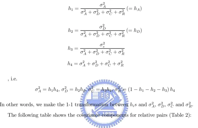
Performing the above estimations involves h(k)_A and h(k)_D ,where k = 1, 2, that are related with σ2

A, σ2D, σ2C and σ2R. To construct their relationship exactly, we let

h1 = σ2 A σ2 A+ σ2D+ σ2C+ σ2R (= hA) h2 = σ2 D σ2 A+ σ2D+ σ2C + σ2R (= hD) h3 = σ2 c σ2 A+ σ2D+ σ2C + σ2R h4 = σ2A+ σ 2 D+ σ 2 C + σ 2 R , i.e. σ2_A= h1h4, σ2D = h2h4, σC2 = h3h4, σ2R= (1− h1− h2− h3) h4

In other words, we make the 1-1 transformation between his and σ2A, σ2D, σ2C and σ2R. The following table shows the covariance components for relative pairs (Table 2):

Table 2. The covariance components for relative pairs

Relationship Covariance V=Covariance after transformation

Same person σ2 A+ σ2D+ λσ2C + σ2R h1h4+ h2h4+ λh3h4+ (1− h1− h2− h3) h4 Parent-child 1₂σ2 A+ λσ2C 1 2h1h4+ λh3h4 Full sibling 1₂σ2 A+ 1 4σ 2 D+ λσ2C 1 2h1h4+ 1 4h2h4+ λh3h4 Half sibling 1₄σ2 A+ λσ2C 1 4h1h4+ λh3h4 Monozygous twins σ2 A+ σ2D+ λσ2C h1h4+ h2h4+ λh3h4 Grandparent-grandchild 1₄σ2A+ λσ2C 14h1h4+ λh3h4 Uncle/aunt-nephew/niece 1₄σ2A+ λσ2C 14h1h4+ λh3h4 First cousins 1 8σ 2 A+ λσ2C 18h1h4+ λh3h4 Double first cousins 1₄σ2

A+ 1 16σ 2 D+ λσ2C 1 4h1h4+ 1 16h2h4+ λh3h4 Spoused λσ2 C λh3h4

Theorem 1 Suppose two models are Pij = x0(1)ij β (1) + G(1)_ij + ε(1)_ij and Pij = x0(2)ij β (2) + G(2)_ij + ε(2)_ij ,respectively, where ε(t)_{ij ∼ N}³0, (σ2R) (t)´ ≡ N³0,³1_{− h}(t)1 − h (t) 2 − h (t) 3 ´ h(t)4 ´ , G(t)_{ij ∼} N ³ 0, (σ2A+ σ2D+ σ2C) (t)´ ≡ N³0, h(t)₁ h(t)4 + h (t) 2 h (t) 4 + h (t) 3 h (t) 4 ´ ,and Cov (Gij, Gik) [j 6= k] = ¡ 2φ_ij,ikσ2 A+ ∆ij,ikσ2D+ λij,ikσ2C ¢t ≡ 2φij,ikh (t) 1 h (t) 4 + ∆ij,ikh (t) 2 h (t) 4 + λij,ikh (t) 3 h (t) 4 . And Pij is the observed value in the jth member of the ith family, xij is his/her corresponding covariate vector. Assumed R is the total number of family and there are ni members in the ith family. Let h(t) ₌³_h(t) 1 , h (t) 2 , h (t) 3 , h (t) 4 ´ , then we have Cov³bh(t)_q , bh(t_q∗∗) ´ ≈ " _R X r=1 (Ã ∂Vr(t) ∂h(t)q !0Ã W−1(t)∂W (t) ∂h(t)q W−1(t) !_³ b S_r(t)_{− b}V_r(t)´ + Ã ∂Vr(t) ∂h(t)q !0 W−1(k) Ã ∂Vr(t) ∂h(t)q !)# × " _R X r=1 (Ã ∂Vr(t) ∂h(t)q !0 W−1(t)³Sbr(t)− bVr(t) ´ ³ b Sr(t∗)− bV(t ∗₎ r ´0 W−1(t∗) Ã ∂Vr(t∗) ∂h(tq∗∗) !)# × " _R X i=1 (Ã ∂Vr(t∗) ∂h(t_q∗∗) !0Ã W−1(t∗)∂W (t∗₎ ∂h(t_q∗∗) W−1(t∗) !_³ b Sr(t∗)− bV(t ∗₎ r ´ + Ã ∂Vr(t∗) ∂h(t_q∗∗) !0 W−1(t∗) Ã ∂Vr(t∗) ∂h(t_q∗∗) !)# q = 1, 2, 3, 4 q∗ = 1, 2, 3, 4 t = 1, 2 t∗ = 1, 2 where Sr(t)= ³ r(t)r1r (t) r1 , r (t) r1r (t) r2 , · · · , r (t) r1r (t) rnr , · · · , r (t) rnrr (t) rnr ´0 , r_rj(t)= Prj − x (t) rjβ (t)_,

V_r(t) = E³S_r(t); β(t), h(t)´ as given by Covariance after transformation in table I,

W_r×r(t) = ⎧ ⎪ ⎨ ⎪ ⎩ 2σ(t)2

ij for the i, jth and l, mth pairs

σ(t)_il σ(t)_im+ σ(t)_imσ(t)_jl for the i, jth and l, mth pairs

and ∂W (t) ∂h(t) = ⎧ ⎪ ⎨ ⎪ ⎩ 4σij ∂σij

∂h for the i, jth and l, mth pairs

∂σil ∂h σjm+ σil ∂σjm ∂h + ∂σim ∂h σjl+ σim ∂σjl

∂h for the i, jth and l, mth pairs In the theorem, both Sr(t) and Vr(t) are vectors which their length are

h³nr 2 ´ + nr i , and W_r×r(t) is ah³nr 2 ´ + nr i ×h³n₂r´+ nr i matrix.

Proof. See Appendix. In the procedure, we have used Generalized Estimating Equations (GEE) method [Zeger and Liang, 1992; Amos, 1994], Taylor’s expansion and some matrix operation [Harville, 1997].

In our situation, W(t) , W(t∗) and ∂W (t) ∂h(t)q

need to estimate. We estimate them with cW(t) , c W(t∗) and ∂W\ (t) ∂h(t)q , where cW(t) , cW(t∗) and ∂W\ (t) ∂h(t)q

are combination of bh1 , bh2 , bh3 and bh4 . h1 and h2 are of our interest, so we only focus on the derivative of covariance components, related h1 and h2., for relative pairs. The following table shows the interested derivative of covariance components for relative pairs (Table 3):

Table 3. The derivative of covariance components for relative pairs

Relationship ∂V ∂h1 ∂V ∂h2 ∂ eV ∂h1 ∂ eV ∂h2 Same person 0 0 0 0 Parent-child 1₂h4 0 1₂ 0 Full sibling 1 2h4 1 4h4 1 2 1 4 Half sibling 1 4h4 0 1 4 0 Monozygous twins h4 h4 1 1 Grandparent-grandchild 1₄h4 0 1₄ 0 Uncle/aunt-nephew/niece 1₄h4 0 1₄ 0 First cousins 1₈h4 0 1₈ 0

Double first cousins 1₄h4 ₁₆1 h4 1_{4 16}1

Corollary 2 Based on table 3, we can express the result of theorem 1 as follow: Cov³bh(t)_q , bh(t_q∗∗) ´ ≈ " _R X r=1 ( bh(t) 4 Ã ∂ eVr(t) ∂h(t)q !0Ã W−1(t)∂W (t) ∂h(t)q W−1(t) !_³ b S_r(t)_{− b}V_r(t)´ + bh(t)₄ Ã ∂ eVr(t) ∂h(t)q !0 W−1(k) Ã ∂ eVr(t) ∂h(t)q ! bh(t) 4 )# × " _R X r=1 ( bh(t) 4 Ã ∂ eVr(t) ∂h(t)q !0 W−1(t)³Sbr(t)− bVr(t) ´ ³ b Sr(t∗)− bV(t ∗₎ r ´0 W−1(t∗) Ã ∂ eVr(t∗) ∂h(tq∗∗) ! bh(t∗₎ 4 )# × " _R X i=1 ( bh(t∗₎ 4 Ã ∂ eVr(t∗) ∂h(tq∗∗) !0Ã W−1(t∗)∂W (t∗₎ ∂h(tq∗∗) W−1(t∗) !_³ b Sr(t∗)− bV(t ∗₎ r ´ + bh(t4∗) Ã ∂ eVr(t∗) ∂h(tq∗∗) !0 W−1(t∗) Ã ∂ eVr(t∗) ∂h(tq∗∗) ! bh(t∗₎ 4 )# q = 1, 2, 3, 4 q∗ = 1, 2, 3, 4 t = 1, 2 t∗ = 1, 2 In our case, Ã ∂ eVr(t) ∂h(t)q ! = Ã ∂ eVr(t∗) ∂h(t_q∗∗) ! when q = q∗ _{, where t = 1, 2; t}∗ _{= 1, 2.}

Corollary2 is almost same with Theorem1 in its form. But one of the advantage of Corol-lary2 is that the time of performing the program in the computer is less than Theorem1.

Now, let two models be

Pij = αH+ γHEij+ τHZij + Gij + ≡ x0(1)ij β (1)_{+ G}(1) ij + ε (1) ij and Pij = αH+ τHZij + Gij + ≡ x0(2)ij β (2)_{+ G}(2) ij + ε (2) ij

Under the same assumptions, we can apply above Theorem1 or Corollary2 to compute some needful estimators for using Fieller’s theorem or delta method. Moreover, we can obtain the confidence limits of P HE or the estimator of deviation of P HE to perform a statistical test or to establish some criteria for determining whether E is an endophenotye.

3.3

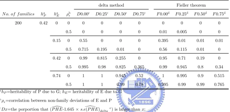
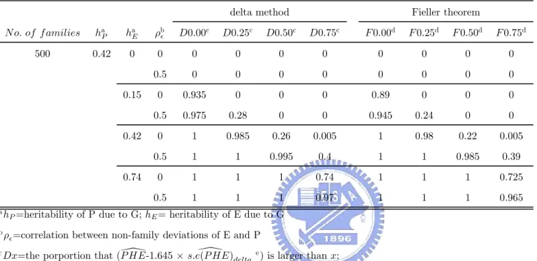
For having more statistical meanings of P HE, we utilize the confidence interval to get more informations about P HE. We hope to find a value that it means there exist a useful endophenotype when PHE value is larger than the value. That is, do one-sided confidence interval, corresponding to such test,

⎧ ⎪ ⎨ ⎪ ⎩ H0 : P HE = a H1 : P HE > a

Under significance α, we reject H0 if the lower bound of one-sided confidence interval of P HE, \

P HE_{− Z1−α × s.e.}³P HE\´_{, is larger than a. However, we get the 100 (1 − α) % confidence} limits of P HE when Fieller’s Theorem was used. So we take the lower bound of confidence limits of 100 (1 − 2α) % as the lower bound of 100 (1 − α) % one-sided confidence interval. In our following simulation, we considered some different values of the cutpoint, a. Under α=0.05, we calculated the proportion that (\P HE_{− 1.645 ×}s.e (P HE)\ _delta) is larger than 0, 0.25, 0.50 and 0.75 respectively, wheres.e (P HE)\ _delta is the estimator of s.e.³P HE\´by using delta method, and the proportion that the lower bound of 95% one-sided confidence interval with using Fieller theorem is larger than 0, 0.25, 0.50 and 0.75 respectively. Based on different values of the cutpoint in our simulation, we hope to construct some criteria to help us validate useful endophenotypes.

4

SIMULATION STUDIES

4.1

The simulation studies evaluate the utility of the proposed index, PHE, under two different scenarios (Figure 2). In Scenario I, the disease gene has a direct effect on phenotype and endophenotype. Scenario II allows multiple disease genes. At the same time, we try to show the relationship between the PHE values and the LOD-score curve. The study design is as follows. There are five markers, each marker has five allele, each allele has population frequency

0.2, and they are on the same chromosome with each of the four intervals between adjacent markers being 10 cM. The disease gene is located at the midpoint of the second interval and has two alleles. The population frequency of most common allele was 0.9. With SIMULATE [Ott 2002], that is a computer program originally written by Joseph Terwilliger, the loci of the markers and the disease gene were simulated based on above description.

Our simulations assumed both endophenotype and phenotype to be continuous measure-ments. The quantitative trait y and genes that influence it were assumed to have a linear relation as described in Almasy and Blangero [1998]:

y = μ + n X

i=1

η_i+ ,

where μ was the grand mean, ηi was the random effect of the ith disease gene, and rep-resented a random non-family deviation. ηi and were assumed to be normally distributed and uncorrelated. For these simulations, dominance effects and shared environmental effects were not included, and therefore var(η_i) = σ2

Ai . For scenario I, each of E (endophenotype) and P (phenotype) was generated to have the single-gene contribution from G (disease gene) simulated by SIMULATE. The non-family deviation of E ( E) and the non-family deviation of P ( P) were assumed to have a correlation ρ . The multiple gene effect in scenario II included the action of gene G1 (disease gene) on E and P , the single-gene action of G2 on E and the single-gene action of G3 on P .

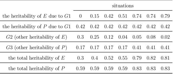
The simulated data contained either 200 or 500 unclear families, and two sibships were generated for each family. In scenario I, the heritability of P due to G was assumed to be 0.42, and the heritability of E due to G allowed being 0, 0.15, 0.42 or 0.74. The correlation between non-family deviations of E and P , ρ , was 0, or 0.5. In scenario II, there are two situations under our consideration. One is that the total heritability of P is larger than the total heritability of E, the other is, on the contrary, the total heritability of P is smaller than

the total heritability of E. The parameter values were shown as the following tables:

Table 4. the total heritability of P > the total heritability of E situations

the heritability of E due to G1 0 0.15 0.42 0.51 0.74 0.74 0.79

the heritability of P due to G1 0.42 0.42 0.42 0.42 0.42 0.42 0.42

G2 (other heritability of E) 0.3 0.25 0.12 0.04 0.05 0.08 0.02

G3 (other heritability of P ) 0.17 0.17 0.17 0.17 0.41 0.41 0.41

the total heritability of E 0.3 0.4 0.52 0.55 0.79 0.82 0.81

the total heritability of P 0.59 0.59 0.59 0.59 0.83 0.83 0.83

Table 5. the total heritability of P < the total heritability of E situations

the heritability of E due to G1 0 0.15 0.42 0.62 0.74 0.74

the heritability of P due to G1 0.42 0.42 0.42 0.42 0.42 0.42

G2(other heritability of E) 0.7 0.59 0.23 0.23 0.08 0.21

G3(other heritability of P ) 0.17 0.17 0.17 0.17 0.17 0.17

the total heritability of E 0.7 0.74 0.65 0.85 0.82 0.95

the total heritability of P 0.59 0.59 0.59 0.59 0.59 0.59

The correlation between non-family deviations of E and P , ρ , was the same as scenario I. Two hundred replications were performed for each specified situation. For simplicity, we denote the coordinates, (fam, h(G1E), h(G1P), h(G2E), h(G3P), ρ ), to express these parameters in each situation, where fam means the numbers of family members, h(G1E)means the heritability of E due to G1, h(G1P)means the heritability of P due to G1, h(G2E)means other heritability of E due to G2, h(G2E)means other heritability of P due to G3, and ρ means the correlation between non-family deviations of E and P . We can find scenario I is a special case of scenario II if h(G1) = G , h(G2E) = 0 , and h(G3p) = 0 in the coordinates’ expression, where G is a single-gene (disease gene) in scenario I.

The computer package SOLAR (Sequential Oligogenic Linkage Analysis Routines) [Blangero et al, 2004; Almasy and Blangero, 1998] was used. The SOLAR command “simqtl” was used to simulate the data following two scenarios. The variance component analysis (24) was performed using the SOLAR command “polymod”. Besides, we use the SOLAR command “multipoint” to create the LOD-score. Before using the SOLAR command “multipoint”, we must set chromosome information about our markers. We set 0cM, 10cM, 20cM, 30cM and 40cM as the positions of the markers in the chromosome respectively, that is, we hoped that there is a high LOD-score peak at 15cM to find the disease gene. Also, the estimates of the standard error of PHE was calculated by using R software. And we plot the mean LOD-score curve according as the results from 200 replications.

4.2

Table 6-9 contain results under scenario I. Table 10-13 contain results under scenario II with the total heritability of P > the total heritability of E and Table 14-17 contain results under scenario II with the total heritability of P < the total heritability of E.

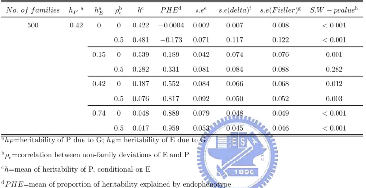
4.2.1 PHE

Table 6 and Table 7 contain results under the ideal causal relation (scenario I). The her-itability of P due to G was fixed. The higher the herher-itability of E due to G, the lower the heritability of P conditional on E and the closer the P HE values to 1. No matter that we chose the correlation between non-family deviations of E and P is either 0 or 0.5, the trend is still kept.

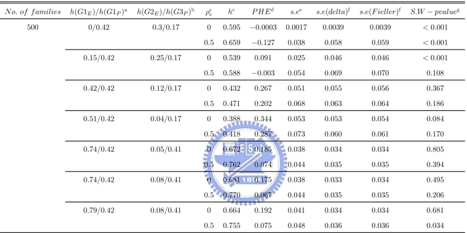
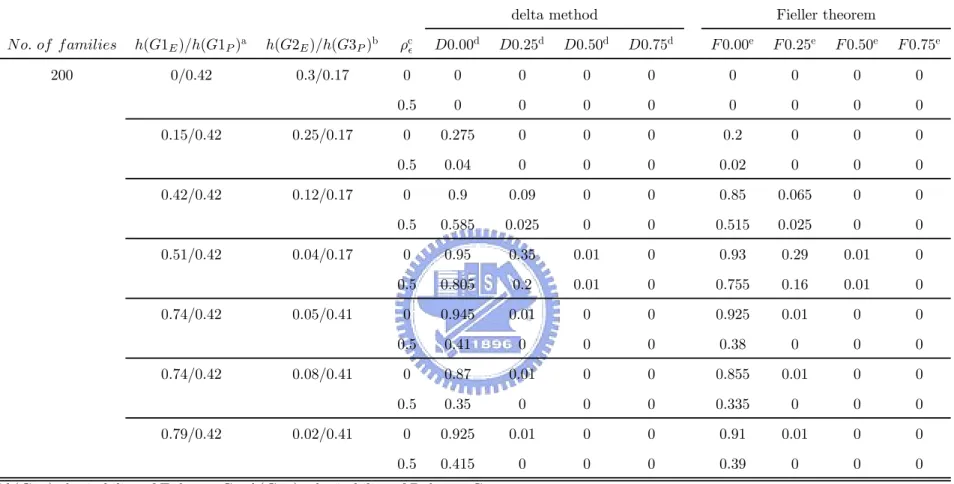
Table 10 and Table 11 show the results when there exist multiple disease genes under scenario II with the total heritability of P > the total heritability of E. When the heritability of P due to G1 were fixed as 0.42 and the heritability of P due to G3 were fixed as 0.17 or 0.41, the trend, that the higher the heritability of E due to G1, the higher the P HE values, is consistent with scenario I. Under scenario II with the total heritability of P < the total heritability of E, Table 14 and Table 15 show a similar trend between the heritability of E due to G1 and P HE. However, we can find these values, the heritability of P due to G3 and

the heritability of E due to G2, also influence the P HE values. The higher the heritability of P due to G3 or the heritability of E due to G2, the lower the P HE values. Besides, the involvement of ρ = 0.5 leads the P HE values to be disrupted. That is, it reduces the efficiency to use the PHE values for searching a useful endophenotype.

4.2.2 THE ACCURACY OF THE ESTIMAOERS OF THE STANDARD ERROR

OF PHE

To check the accuracy of the estimators of the standard error of P HE calculated according to the delta method or the Fieller’s theorem and our provided theorem or corollary, we compare the standard error of proportion of heritability explained by endophenotype(s.e) that was simulated with s.e(delta) and s.e(Fieller), where s.e(delta) is the mean of estimator of s.e by using delta method and s.e(Fieller) is the mean of the range of 95% confidence limits of PHE, used by Fieller method, divided by 2 × 1.96. Table 6, Table 7, Table 10, Table 11, Table 14 and Table 15 contain these results under scenario I and scenario II. Let us regard the standard error of proportion of heritability explained by endophenotype(s.e), that was simulated, as the true standard deviation of proportion of heritability explained by endophenotype. We can find that, when the heritability of E due to the disease gene is lower than the heritability of P due to the shared gene, s.e(delta) and s.e(Fieller) tend to be overestimated. And s.e(delta) and s.e(Fieller) tend to be underestimated when the heritability of E due to the disease gene is higher than the heritability of P due to the shared gene. Also, we find that the relative error of the overestimators is larger than the relative error of the underestimators. But both the absolute error of the overestimators and the underestimators are small. That is, these estimators of the standard error of P HE are closer the true standard error of P HE. However, using these estimators calculated by either delta method or Fieller theorem don’t have too wide confidence interval of P HE to make some statistical inferences. In other words, these estimators can be allowed.

4.2.3 TEST OF PHE

For using normal distribution to perform statistical tests or establish a confidence interval of P HE, we used Shapiro-Wilk statistic to test the normality of P HE. Table 6, Table 7, Table 10, Table 11, Table 14 and Table 15 also shows these p-values of using Shapiro-Wilk test under scenario I and scenario II. The histograms of PHE values under different situations are shown in Figure 3-14. Under scenario I, the normality of PHE doesn’t hold in most situations. But the normality of P HE holds in most situations under scenario II. In other words, although using normal distribution is not good , it isn’t too bad. Briefly, using normal distribution can be acceptable with a lower standard..

We first describe the information about the mean LOD-score curve under both scenario I and scenario II (Figure 15-26). The LOD-score in our simulation was found to be related to the number of families and the heritability of the trait due to the common disease gene, where the trait may be a phenotype or an endophenotype. When the heritability of the endophenotype due to the common disease gene is larger than the heritability of the phenotype due to the common disease gene, the endophenotype is useful to search the disease gene. We except that the heritability of the endophenotype due to the common disease gene isn’t smaller than the heritability of the phenotype due to the disease gene. These results were consistent to the results from other papers [Almasy and Blangero, 1998; Williams et al., 1999].

Table 8 and Table 9 contain results under scenario I. At the same time, Figure 15, Figure 16, Figure 17 and Figure 18 show the mean LOD-score curve under scenario I. Based on these figures, when the heritability of P due G was assumed to be 0.42 and the heritability of E due to G allowed being 0 and 0.15, we find that using endophenotype to search for the disease gene is worse than using phenotype because the mean LOD-score of P was higher than the mean LOD-score of E. That is, we don’t hope that these are endophenotypes. On the other hand, when the heritability of P due to G was assumed to be 0.42 and the heritability of E due to G was assumed to be 0.74, endophenotype-based genetic analysis is more likely to succeed than one in terms of search for the disease gene (i.e. the mean LOD-score of E is higher than the one of P ). Besides, when the heritability of P due to G was assumed to be 0.42 and the heritability of E due to G was assumed to be 0.42, the phenotype-based effect

and the endophenotype-based effect are same. Altogether, when the heritability of P due to G was assumed to be 0.42 and the heritability of E due to G was assumed to be 0.42 or 0.74, the endophenotype-based effect isn’t worse than the phenotype-based effect. As a result of above descriptions about mean LOD-score curve, based on Table A3 and Table A4, we view it endophenotype candidate if lower bound of 95% one-sided confidence interval is larger than 0.25 or 0.50. The criterion that lower bound of 95% one-sided confidence interval is larger than 0.50 can be seen as a stronger evidence and the criterion that lower bound of 95% one-sided confidence interval is larger than 0.25 is also a suitable frame of reference. With another viewpoint, using two cutpoints, 0.25 and 0.50, the power, that the probability of rejecting H0 when H1 holds, will exceed 0.7 or 0.8 except for the situation where the heritability of P due to G was assumed to be 0.42, the heritability of E due to G was assumed to be 0.42, ρ was assumed to be 0, and cutpoint is set as 0.50. It implies that endophenotype-based effect isn’t worse than the phenotype-based effect. If it is desired that there is a higher power such as 0.9, 0 may be an applicable cutpoint no matter ρ was either 0 or 0.5. But it also leads the result ,that endophenotype-based effect is worse than the phenotype-based effect, happen, such as the situation where the heritability of P due G was assumed to be 0.42 and the heritability of E due to G allowed being 0.15.

In scenario II, on account of disrupted P HE values with the heritability of P due to G3 and the heritability of E due to G2, the criteria under scenario I may become improper. Based on Table 12, Table 13, Table 16 and Table 17, we downscale the standard of these criteria for searching the endophenotype successfully. The criterion that lower bound of 95% one-sided confidence interval is larger than 0.25 is still a suitable one. But many useful endophenotypes will be missed. So, we find that the criterion that lower bound of 95% one-sided confidence interval is larger than 0 should be seen as the criterion that search the potential candidate of endophenotype. Furthermore, if we want to let the higher power be kept for the goal that endophenotype-based effect isn’t worse than the phenotype-based effect, considered cutpoint may be 0. However, if ρ was assumed to be 0.5, the chosen cutpoint, 0, is not sufficient because of the lower power.

95% one-sided confidence interval is larger than 0 is the potential evidence for searching the endophenotype. The second criterion that lower bound of 95% one-sided confidence interval is larger than 0.25 is the moderate evidence for searching the endophenotype. And the third criterion that lower bound of 95% one-sided confidence interval is larger than 0.50 is the stronger evidence for searching the endophenotype. However, you can choose some different criteria depended on the different goals of different cases or use lower bound of 95% one-sided confidence interval directly as the evidence for searching the endophenotype.

In another aspect, using the viewpoint of "power", we try to construct some steps to help us determine the desired endophenotype. The process of our construction is as follows. At the first step, check if ρ is 0 because it brings different information about use of the PHE values. If it doesn’t hold, we are careful with use of P HE values because there is a lower power of detecting the useful endophenotypes if ρ is 0.5 even when the cutpoint is set as 0. That is, the involvement of ρ 6= 0 leads much uncertainty to use PHE values. Furthermore, if ρ become larger, using the PHE values may loss much useful information of the endophenotypes. In other words, If the lower bound of 95% one-sided confidence interval isn’t larger than 0 when ρ is larger than 0, it doesn’t imply that the endophenotype is helpless. If ρ is 0, we will perform the second step.

At the second step, check if the lower bound of 95% one-sided confidence interval is larger than 0.25. If it holds, it implies two possibilities : (1) there is the single disease gene to lead a direct effect on phenotype and endophenotype such as Scenario I and endophenotype-based effect isn’t worse than the phenotype-based effect; (2) it implies that both the influences of other genes on phenotype and endophenotype can be small, relative to the influences of the shared genes on phenotype and endophenotype such as Scenario II and endophenotype-based effect is better than the phenotype-based effect. If the lower bound of 95% one-sided confidence interval isn’t larger than 0.25, we will proceed to perform the third step.

At the third step, check if the lower bound of 95% one-sided confidence interval is larger than 0. If it holds, there exists two possible situations : (1) there is the single disease gene to lead a direct effect on phenotype and endophenotype such as scenario I and endophenotype-based effect isn’t better than the phenotype-endophenotype-based effect. It is out of our desire; (2) the

influence of other genes of either phenotype or endophenotype can be large relatively to the influence of the shared genes of either phenotype or endophenotype respectively such as sce-nario II and endophenotype-based effect isn’t worse than the phenotype-based effect. If the lower bound of 95% one-sided confidence interval isn’t larger than 0 when ρ is 0, it means there is a high probability that it isn’t a useful endophonotype. In sum, using three steps is helpful to search a useful endophenotype.

5

DISCUSSION

Based on definition of an endophenotype proposed by Huang et al. [2005], we have at-tempted to provide criteria that can be used to validate an endophenotype. Huang et al.,2005 had shown that the proposed index, P HE, is useful in validating endophenotypes. In our re-port, we use P HE proposed by Huang et al. [2005] as the index for evaluating endophenotypes to provide more clear informations, three criteria and three steps, through the one-sided con-fidence interval or the statistical test. However, we can find that the more the total numbers of family members, the more efficiency of detecting a useful endophenotype.

As discussed in corresponding index for validating surrogate endpoints such as P T E, con-fidence intervals of P T E can be calculated using Fieller’s theorem [Buyse and Molenberghs, 1998], however, they are usually too wide to be useful. With our proposed theorem or corol-lary, we use Fieller’s theorem or delta method to calculate confidence intervals of P HE. Our simulation results show that the estimators of standard error of P HE values’ estimators are near “true” standard errors of these indices’ estimators. That is, they are quite reasonable to avoid too wide confidence interval to be useful. However, although they may be overestimated or underestimated , they are helpful to detect the useful endophenotype easily. This is be-cause that it tends to have a underestimator of standard error of P HE estimator for the good endophenotype and it leads the lower bound of 95% one-sided confidence interval to be easily larger than our set cutpoint. Otherwise, the lower bound of 95% one-sided confidence interval tend to be smaller than our set cutpoint for the useless endophenotype. In other words, it isn’t too serious for using these overestimated or underestimated estimators of standard error of

P HE values’ estimators to construct a reasonable one-sided confidence interval and to search a useful endophenotype.

Besides, our simulation results show that the multiple gene effect lowers P HE values to lead it confused for evaluating endophenotypes. We provide three criteria and three steps to help us understand the pattern of P HE values versus the relationship between endophenotype and phenotype. If you aren’t interested in the relationship between P HE values and the heritabilities caused by different genes, the second step can be omitted. However, among three steps, we need to check that ρ is 0. The SOLAR command "polygenic" can be used to calculate ρ . If ρ is near 0, we can view it 0 to use three criteria and three steps safely for searching a useful endophenotype. Furthermore, at the third step, we will face the situation that the influence of other genes of either phenotype or endophenotype can be large relatively to the influence of the shared genes of either phenotype or endophenotype respectively such as Scenario II. For the influence of other genes of phenotype or endophenotype, we can use linkage analysis to determine which heritability is relatively large. If the heritability of other genes of phenotype is relatively large to the heritability of the found disease gene of phenotype, it means that only using an endophenotype may be sufficient. We must to search more than one endophenotype to capture a complete feature of the specified phenotype. The following model can be tried to be considered.

P = αH+ γ1HE1 + γ2HE2 + τHZ + G + ,

where E1 is assumed to being a found endophenotype and E2 is assumed to being a new or interested endophenotype. And we calculate the P HE value, 1 − h_hE1E2

N E

, directly and its lower bound of 95% one-sided confidence interval, where hE1E2 is the heritability calculated from the variance component analysis (24) including the endophenotypes, E1 and E2, with any other covariates. To avoid to get same information or to find similar endophonotypes, we also calculate the partial proportion of heritability explained (P P HE) by the endophenotype defined as

P P HE = 1₋ hE1E2 hE1

where hE1E2 is the heritability calculated from the variance component analysis (24) including the endophenotypes, E1 and E2, with any other covariates and hE1 is the heritability cal-culated from the variance component analysis (24) without including the endophenotype E2 with any other covariates. A good and new endophenotype is one that explains a large pro-portion of heritability given a found endophenotype E1, thus, the greater the P P HE value, the more likely E2 an desired endophenotype.

In the future, to make it clear for using the P HE values, especially when ρ 6= 0, we should simulate with ρ < 0 and ρ >> 0. The information of the P HE values involved with negative ρ is a loss of our report. However, the much higher ρ is considered to help us understand the efficiency of using the P HE values to detect a useful endophenotype clearly in a bad situation. If the power of using the P HE values to detect useful endophenotype candidates isn’t too low when ρ is a much larger value, P HE values will be very useful index to search a useful endophenotype to increase opportunities of finding susceptible disease genes.

Appendix: Let model1: Pij = x0(1)ij β (1)_{+ G}(1) ij + ε (1) ij and model2: Pij = x0(2)ij β (2)_{+ G}(2) ij + ε (2) ij ,where ε(t)_{ij ∼ N}³0,¡σ2_R¢(t)´_{≡ N}³0,³1_{− h}(t)_{1 − h}(t)_{2 − h}(t)₃ ´h(t)₄ ´ G(t)_{ij ∼ N}³0,¡σ2_A+ σ2_D+ σ2_C¢(t)´_{≡ N}³0, h(t)₁ h(t)₄ + h(t)₂ h(t)₄ + h(t)₃ h(t)₄ ´ Cov (Gij, Gik) [j 6= k] = ¡ 2φij,ikσ 2 A+ ∆ij,ikσ2D+ λij,ikσ2C ¢t ≡ 2φij,ikh (t) 1 h (t) 4 + ∆ij,ikh (t) 2 h (t) 4 + λij,ikh (t) 3 h (t) 4 t = 1, 2

By GEE [Zeger and Liang, 1992; Amos, 1994],

S_β(t) ³ β(t), h(t)´= R X r=1 Ã ∂Xr(t)β(t) ∂β(t) !0 Cov−1(Pr) ³ Pr− Xr(t)β (t)´ = 0 where Pr= (Pr1 , · · · , Prnr)0, and X (t) r = ³ x(t)_{r1 , · · · , x}(t)rnr ´0 .

The correlation parameter h may be estimated by simultaneously solving

S_β(t) ³ β(t), h(t)´= 0 and Sh(t) ³ β(t), h(t)´= R X r=1 Ã ∂Vr(t) ∂h(t) !0 W−1(t)¡Sr(t)− Vr(t) ¢ = 0 where S_r(t)=³r_r1(t)r_r1(t) , r_r1(t)r_r2(t) _{, · · · , r}(t)_r1r_rnr(t) _{, · · · , r}(t)_rnrr(t)_rnr´0, r(t)_rj = Prj − x0(t)rj β (t) , Vr(t) = E ³ Sr(t); β (t)

and W_r×r(t) = ⎧ ⎪ ⎨ ⎪ ⎩

2σ(t)ij2 for the i, jth and l, mth pairs

σ(t)_il σ(t)_im+ σ(t)_imσ(t)_jl for the i, jth and l, mth pairs

. Since Sh(t) ³ β(t), h(t)´= R X r=1 à ∂Vr(t) ∂h(t) !0 W−1(t)¡Sr(t)− Vr(t) ¢ and ∂2_V(t) r ∂ (h(t)₎2 = 0, we have S_h(t) ³ β(t), h(t)´ ∂h(t) = R X r=1 "à ∂Vr(t) ∂h(t) !0à ∂W−1(t) ∂h(t) ! ¡ Sr(t)− V (t) r ¢ + à ∂Vr(t) ∂h(t) !0 W−1(t) à −∂V (t) r ∂h(t) !# = R X r=1 "à ∂Vr(t) ∂h(t) !0µ −W−1(t)∂W (t) ∂h(t) W −1_(t)¶¡ S_r(t)_{− Vr}(t)¢+ à ∂Vr(t) ∂h(t) !0 W−1(t) à −∂V (t) r ∂h(t) !# . where ∂W(t) ∂h(t) = ⎧ ⎪ ⎨ ⎪ ⎩ 4σij ∂σij

∂h for the i, jth and l, mth pairs

∂σil ∂h σjm+ σil ∂σjm ∂h + ∂σim ∂h σjl+ σim ∂σjl

∂h for the i, jth and l, mth pairs Using Taylor’s expansion, we have

bh(k) − h(k) = à _R X r=1 "à ∂Vr(t) ∂h(t) !0µ −W−1(t)∂W (t) ∂h(t) W −1_(t)¶¡ Sr(t)− Vr(t) ¢ + à ∂Vr(t) ∂h(t) !0 W−1(t) à −∂V (t) r ∂h(t) !#!−1 × Ã _R X r=1 à ∂Vr(t) ∂h(t) !0 W−1(t)¡S_r(t)_{− Vr}(t)¢ !

Cov³bh(t)_q , bh(t_q∗∗) ´ = Cov ³ bh(t) q − h (t) q , bh (t∗₎ q∗ − h (t∗₎ q∗ ´ = Cov ( à _R X r=1 "à ∂Vr(t) ∂h(t)q !0à −W−1(t)∂W (t) ∂h(t)q W−1(t) ! ¡ S_r(t)_{− Vr}(t)¢ + à ∂Vr(t) ∂h(t)q !0 W−1(t) à −∂V (t) r ∂h(t)q !#!−1 × Ã _R X r=1 à ∂Vr(t) ∂h(t)q !0 W−1(t)¡S_r(t)_{− Vr}(t)¢ ! , à _R X r=1 "à ∂Vr(t∗) ∂h(tq∗∗) !0à −W−1(t∗)∂W (t∗₎ ∂h(tq∗∗) W−1(t∗) ! ¡ Sr(t∗)− V(t ∗₎ r ¢ + à ∂Vr(t∗) ∂h(t_q∗∗) !0 W−1(t∗) à −∂V (t∗₎ r ∂h(t_q∗∗) !#!−1 × Ã _R X r=1 à ∂Vr(t∗) ∂h(t_q∗∗) !0 W−1(t∗)¡S_r(t∗)_{− Vr}(t∗)¢ ! ⎫_⎬ ⎭ Note that à _R X r=1 "à ∂Vr(t) ∂h(t)q !0à −W−1(t)∂W (t) ∂h(t)q W−1(t) ! ¡ S_r(t)_{− Vr}(t)¢+ à ∂Vr(t) ∂h(t)q !0 W−1(t) à −∂V (t) r ∂h(t)q !#!−1 and à _R X r=1 "à ∂Vr(t∗) ∂h(t_q∗∗) !0à −W−1(t∗)∂W (t∗₎ ∂h(t_q∗∗) W−1(t∗) ! ¡ S_r(t∗)_{− Vr}(t∗)¢+ à ∂Vr(t∗) ∂h(t_q∗∗) !0 W−1(t∗) à −∂V (t∗₎ r ∂h(t_q∗∗) !#!−1 are 1 × 1 matrices.

Besides, for simplicity, we can replace them with

à _R X r=1 "à ∂Vr(t) ∂h(t)q !0à −W−1(t)∂W (t) ∂h(t)q W−1(t) !_³ b S_r(t)_{− b}V_r(t)´ + à ∂Vr(t) ∂h(t)q !0 W−1(t) à −∂V (t) r ∂h(t)q !#! and à _R X"Ã∂Vr(t∗) ∂h(t∗∗) !0à −W−1(t∗)∂W (t∗₎ ∂h(t∗∗) W−1(t∗) !_³ b S_r(t∗)_{− b}V_r(t∗)´ + à ∂Vr(t∗) ∂h(t∗∗) !0 W−1(t∗) à −∂V (t∗₎ r ∂h(t∗∗) !#!

then Cov³bh(t)_q , bh(t_q∗∗) ´ ≈ Ã _R X r=1 "Ã ∂Vr(t) ∂h(t)q !0Ã W−1(t)∂W (t) ∂h(t)q W−1(t) !_³ b S_r(t)_{− b}V_r(t)´ + Ã ∂Vr(t) ∂h(t)q !0 W−1(t) Ã ∂Vr(t) ∂h(t)q !#!−1 × " _R X r=1 Cov ÃÃ ∂Vr(t) ∂h(t)q !0 W−1(t)¡S_r(t)_{− Vr}(t)¢, Ã ∂Vr(t∗) ∂h(tq∗∗) !0 W−1(t∗)¡S_r(t∗)_{− Vr}(t∗)¢ !# × Ã _R X r=1 "Ã ∂Vr(t∗) ∂h(t_q∗∗) !0Ã W−1(t∗)∂W (t∗₎ ∂h(t_q∗∗) W−1(t∗) !_³ b S_r(t∗)_{− b}V_r(t∗)´ + Ã ∂Vr(t∗) ∂h(t_q∗∗) !0 W−1(t∗) Ã ∂Vr(t∗) ∂h(t_q∗∗) !#!−1

Since W(t) and W(t∗) are symmetric matrices, W−1(t) and W−1(t∗) are also symmetric ma-trices. Above equation can be written as

Cov³bh(t)_q , bh(tq∗∗) ´ ≈ Ã _R X r=1 "Ã ∂Vr(t) ∂h(t)q !0Ã W−1(t)∂W (t) ∂h(t)q W−1(t) !_³ b S_r(t)_{− b}V_r(t)´ + Ã ∂Vr(t) ∂h(t)q !0 W−1(t) Ã ∂Vr(t) ∂h(t)q !#!−1 × " _R X r=1 Ã ∂Vr(t) ∂h(t)q !0 W−1(t)Cov¡S_r(t)_{− Vr}(t), S_r(t∗)_{− Vr}(t∗)¢W−1(t∗) Ã ∂Vr(t∗) ∂h(t_q∗∗) !# × Ã _R X r=1 "Ã ∂Vr(t∗) ∂h(t_q∗∗) !0Ã W−1(t∗)∂W (t∗) ∂h(t_q∗∗) W−1(t∗) !_³ b S_r(t∗)_{− b}V_r(t∗)´ + Ã ∂Vr(t∗) ∂h(t_q∗∗) !0 W−1(t∗) Ã ∂Vr(t∗) ∂h(t_q∗∗) !#!−1 We estimate Cov³Sr(t)− Vr(t), S(t ∗₎ r − V(t ∗₎ r ´ with ³Sbr(t)− bVr(t) ´ ³ b Sr(t∗)− bV(t ∗₎ r ´ , then we