以AFSM為基礎的感測/驅動控制混合程式驗證

國

立

交

通

大

學

資訊科學與工程研究所

碩

士

論

文

以 AFSM 為基礎的感測/驅動控制混合程式驗證

Hybrid Program Verification for AFSM-based

Sensory-Motor Control

研 究 生：龔哲正

指導教授：邵家健 教授

以 AFSM 為基礎的感測/驅動控制混合程式驗證

Hybrid Program Verification for AFSM Based Sensory-Motor

Control

研 究 生：龔哲正 Student：Zhe-Zheng Gong

指導教授：邵家健 Advisor：John Kar-kin Zao

國 立 交 通 大 學

資 訊 科 學 與 工 程 研 究 所

碩 士 論 文

A Thesis

Submitted to Institute of Computer Science and Engineering

College of Computer Science

National Chiao Tung University

in partial Fulfillment of the Requirements

for the Degree of

Master

in

Computer Science

July 2006

Hsinchu, Taiwan, Republic of China

Hybrid Program Verification for AFSM Based Sensory-Motor

Control

Student：Zhe-Zheng Gong Advisors：John Kar-kin Zao

Institute of Computer Science and Engineering

National Chiao Tung University

ABSTRACT

In this thesis, we develop a method to apply formal verification of Temporal Logic onto an

autonomous robot system controlled by Rodney Brooks’ Augmented Finite State Machine

model.

This method uses some approaches to reduce the complexity of an AFSM-based reactive

robot control system (RRCS), so that verification of AFSM-based RRCS can become

applicable. These approaches applied onto verification include ： (1) State Space

Discretization──It is not feasible to verify a system on continuous space-time domain.

Therefore, before constructing an AFSM-based RRCS we must transform the system and

environment from continuous space domain to discrete space domain. (2) External

function──By exporting internal states and kinematic computation of the robot from the

model checker using the external function provided by OMocha temporal logic model checker.

(3) Elimination of some checking cases──Based on the properties we want to check, we can

eliminate some unnecessary checking cases which will never violate the properties.

After using above-mentioned approaches, the results show that the number of all reachable

states checked by OMocha and checking time improve greatly.

In this thesis, we reach some accomplishments listed below：

(1) Check the Behaviors of the AFSM-based RRCS by Model Checker──After constructing

the AFSM-based RRCS, we describe the “No Collision” property by Temporal Logic, and

two-dimensional environment.

(2) Improve the Performance of Checking Procedure──After reducing the checking time by

the three approaches, the best results show that the checking procedure can be completed in

reasonable time.

According to the accomplishments, we can prove that it’s applicable to apply verification

以 AFSM 為基礎的感測/驅動控制混合程式驗証

學生：龔哲正 指導教授：邵家健

國立交通大學資訊科學與工程研究所 碩士班

摘 要

在這篇論文中，我們發展一個方式將時序邏輯正規驗證法，應用在由 Rodney Brooks 所提出的增強化有限態機器(AFSM)所控制的自主性機器人上。 在這個方式中，我們使用了一些方法去簡化以 AFSM 為基礎的感應式機器控制系統 (RRCS)的複雜度，讓以 AFSM 為基礎的 RRCS 之驗證能夠有可行性。這些被應用在驗證上 的方法包括有：(1)狀態空間離散化──驗證一個在連續定義域上的系統是不可行的。 因此，在建構一個以 AFSM 為基礎的 RRCS 之前，我們必須將系統及環境從連續定義域轉 換到分散定義域。(2)外部函數──藉由 OMocha 所提供的外部函數，將系統中的內部狀 態及運動學上的計算從驗證器中輸出至外部函數。(3) 去除掉不必要的檢驗部分──根 據我們所要檢驗的行為特性，我們能夠將必定不會違背此特性的一些檢驗部分去除掉。 在運用了上述的這些方法後，結果中顯示，被 OMocha 檢驗的全部可到達狀態數目及 檢驗時間都改善了很多。 在這篇論文中，我們將達成的一些成果列在下面： (1)用檢驗器檢驗以 AFSM 為基礎的 RRCS 之行為特性──在建構起以 AFSM 為基礎的 RRCS 後，我們用時序邏輯來描述＂No_Collision＂這個特性，並且證明了被此 RRCS 控制的 機器人在二維空間中將永遠不會碰到障礙物。 (2)改善檢驗程序的效率──在藉由三個方法來縮短檢驗時間後，最佳的結果中顯示檢 驗程序能夠在合理的時間內被完成。

致謝

論文定稿後，我自己重新將論文看了一遍，其中有很多不夠完美的地方，但相信我有 盡我所能去做到最好，希望所有在過程中給予我幫助的大家能夠滿意這篇論文所呈現出 來的樣貌，這是我唯一能夠回報的。 首先，要感謝邵家健教授不斷耐心地給予我指導，雖然老師講的有些東西我好像永遠 沒有弄懂，但我已經從我弄懂的事情中獲得了很多，那已經很足夠了，對於研究、對於 人生，您都是我的良師益友。另外，很感激王柏堯老師及黃耿典學長的協助，希望這次 的合作成果能夠讓你們滿意，也期望將來能繼續合作將這個題目延伸發展下去。再來， 要謝謝實驗室所有的同伴們，過程中互相打氣激勵是一個很重要的動力，在好的研究環 境中才會有好的研究成果，很慶幸能夠和大家一起努力，一同營造出這樣一個令人感到 舒服有鬥志的氛圍。 最後，要感謝我的父母，謝謝你們的栽培，相信你們看不懂這篇論文，不過其中的每 一字一句都是因為你們才存在的。 謝謝大家，也謝謝我自己，辛苦了… 2006/07/26 寫於 620 實驗室

Contents

Abstract……….I 摘要………..III 致謝……….V Contents………..VI List of Figures………...IX List of Tables………XI Chapter 1 Introduction………….………1 1.1 Project Objective………...……….……...1 1.2 Project Approach………...1 1.3 Outline of Thesis………...3

Chapter 2 AFSM-based Reactive Robot Control Systems and Roving Robot Collision Avoidance Experiment………..4

2.1 Augmented Finite State Machine (AFSM) ………4

2.1.1 Why AFSM?...4

2.1.1.1 Simple Procedure for Decomposing and Combining……….4

2.1.1.2 Time Discretization……….5

2.2 Roving Robot Collision Avoidance Experiment ………6

2.2.1 Experiment Overview……….6

2.2.2 Hardware Structure of the Robot………7

2.2.2.1 Sonar Sensors………7

2.2.2.2 Motor………...7

2.2.4 Expected Behaviors of the Experiment………8

2.2.5 Properties To Be Verified………9

Chapter 3 Model Checking for AFSM-based RRCS, Concepts………10

3.1 Checking Procedure………..10

3.1.1 Two Examples of Checking Procedure……….10

3.1.1.1 Simple Example………10

3.1.1.2 Advanced Example………11

3.2 Model Checker：OMocha………..14

3.3 Formal Input Language for OMocha………14

3.3.1 Programs Described by UNITY-based specification language….………14

3.3.2 Properties Described by Temporal Logic………18

Chapter 4 Model Checking for AFSM-based RRCS, Approaches………20

4.1 State Space Discretization……….20

4.2 External Function for Computation/State Hiding……….22

4.2.1 Computation Hiding………..22

4.2.2 State Hiding………...24

4.3 Elimination of Unnecessary Checking Cases………...26

Chapter 5 Implementation of Roving Robot Collision Avoidance Experiment…………27

5.1 Full Structure of the Experiment………...27

5.2 Introduction for each AFSM Module in detail………...29

5.3 Property To Be Verified：”No_Collision” property………...51

Chapter 6 Experiment Results and Analysis………52

6.1 State Hiding Applied to the Experiment………52

6.2 Elimination of Some Checking Cases Applied to the Experiment………53

6.2.1 Principle………53

6.2.3 Approach for Partial Elimination………56

6.2.4 Issue：Unrealistic Cases………57

6.3 Coarse Sampling of States………...57

6.4 Checking Results of the Experiment Applied Different Approaches………58

6.4.1 Case1：Only Apply State Hiding to the Experiment……….59

6.4.2 Case2：Apply State Hiding and Partial Elimination of Checking Cases………...59

6.4.3 C a s e 3 ： A p p l y St a t e H i d i n g a n d S m a r t E l i mi n a t i o n o f C h e c k i n g Cases………60

6.4.4 Case4：Apply State Hiding and Coarse Sampling of States….………...60

6.5 Analysis……….61

Chapter 7 Conclusion……….64

7.1 Accomplishment………...64

7.2 Future Work………...65

List of Figures

Fig. 2-1 Modularized AFSM module………4

Fig. 2-2 Transition function of AFSM module………4

Fig. 2-3 Independent AFSM component………5

Fig. 2-4 The chart of the experiment ……….6

Fig. 2-5 Hardware structure of the robot………7

Fig. 2-6 Environment of the experiment………8

Fig. 3-1 Simple example of AFSM-based system………12

Fig. 3-2 Advanced example of AFSM-based system………13

Fig. 3-3 The trace-tree of verification procedure of advanced example…….14

Fig. 3-4 The trace-tree of verification procedure of simple example……….14

Fig. 3-5 Module description………...15

Fig. 3-6 Example for atoms definition………16

Fig. 3-7 The relationship between latched value and updated value…….17

Fig. 4-1 The relationship between continuous and discrete MAP…………21

Fig. 4-2 An example of the relationship between continuous and discrete domain…21 Fig. 4-3 Encapsulation procedure………25

Fig. 5-1 Full structure of the experiment………....27

Fig. 5-2 MAP module……….29

Fig. 5-3 Some examples for the representation of MAP_obstacle/MAP_wall..30

Fig. 5-4 MAP 1.0………31

Fig. 5-5 UNITY fragment of MAP……….31

Fig. 5-6 SONAR module………...32

Fig. 5-7 Detection range………33

Fig. 5-8 Some examples for the representation of SMAP_obstacle…….33

Fig. 5-9 UNITY fragment of SONAR………34

Fig. 5-10 Fragment of external function detection()……….35

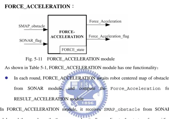
Fig. 5-11 FORCE_ACCELERATION module………..36

Fig. 5-12 The relationship between SMAP_obstacle and Force_Acceleration…37 Fig. 5-13 UNITY fragment of FORCE_ACCELERATION………..38

Fig. 5-14 Fragment of external function SMAP_to_FORCE()………39

Fig. 5-15 RANDOM_ACCELERATION module………..40

Fig. 5-16 The relationship between SMAP_obstacle and Random_Acceleration…41 Fig. 5-17 UNITY fragment of RANDOM_ACCELERATION………..42

Fig. 5-18 RESULT_ACCELERATION module………..42

Fig. 5-19 UNITY fragment of RESULT_ACCELERATION……….44

Fig. 5-21 Some examples of updating Velocity………46

Fig. 5-22 UNITY fragment of VELOCITY……….47

Fig. 5-23 Fragment of external function Update_Velocity()……….48

Fig. 5-24 MOTOR module………49

Fig. 5-25 Some examples of updating Location………49

Fig. 5-26 UNITY fragment of MOTOR………..50

Fig. 5-27 “No_Collision” property checked by OMocha………51

Fig. 6-1 Some variables encapsulated into external function………52

Fig. 6-2 Wandering region………..53

Fig. 6-3 An example for verification procedure………54

Fig. 6-4 The parts of verification procedure can be omitted………54

Fig. 6-5 The partial verification procedure is the collection of checking cases…55 Fig. 6-6 Outward velocities make the robot leave the wandering region………....55

F i g . 6 - 7 T h r e e e x a m p l e s o f c h e c k i n g c a s e s … … … 5 6 Fig. 6-8 All velocities of a state in wandering region………..56

Fig. 6-9 Only half points of wandering region will generate random acceleration...57

List of Tables

Table 3-1 Sequential state transition of simple AFSM-based system………12

Table 3-2 Sequential state transitions of advanced AFSM-based system……….13

Table 5-1 Brief introduction for 7 AFSM modules……….29

Table 5-2 All variables in MAP module………..35

Table 5-3 All variables in SONAR module……….34

Table 5-4 The relationship between “Distance of X-axis away from the obstacle in SMAP_obstacle” and “X-axis component of reverse acceleration degree in Force_Acceleration”………..36

Table 5-5 All variables in FORCE_ACCLERATION module………...38

Table 5-6 All variables in RANDOM_ACCLERATION module………...41

Table 5-7 All variables in RESULT_ACCLERATION module………...44

Table 5-8 All variables in VELOCITY module………...47

Table 5-9 All variables in MOTOR module……….50

Table 5-10 “No_Collision” property……….51

Table 6-1 All parameters of the experiment ………59

Chapter 1

Introduction

1.1 Project Objective

How to write modular reusable programs has always been a major challenge to the

developers of autonomous robots. Rodney Brooks of MIT proposed a new approach, called

Augmented Finite State Machines (AFSM) [1], to program reactive robot control systems (RRCS). The AFSM approach allowed robot programmers to create program modules that

control robot behaviors and develop complex robot behaviors by the composition of these

AFSM modules.

The purpose of this work is to explore the possibility of using formal verification technique

to verify certain properties of the behaviors of AFSM controlled robots. Such a verification

technique will enable robot programmers to test or “debug” their programs before using them

to actually control the robots. The difficulty of this attempt of formal verification lies with the

fact that robot motions are carried out continuously on space and time whereas formal

verification can only be applied onto systems with limited number of discrete states.

Therefore, the challenge is to properly discretize and reduce the number of states of a robot

system so that formal verification can become applicable.

1.2 Project Approach

We explore ways to apply formal verification onto AFSM programs by experimenting with

following approaches/methods.

(A) State Space Discretization

To verify a system on continuous domain is not applicable. Therefore, before constructing

an AFSM-based RRCS we must transform the system and environment from continuous

Discretization, and (2) Space Discretization. After discretization, the number of states of the

system will reduce from infinite to finite so that formal verification can become more

applicable.

(B) Using external function to reduce number of states checked by model checker

External functions are written by high-level language(e.g. C language). For following

reasons, we can use external function to reduce number of states checked by model checker.

(1) During verification procedure, there are some system variables which are irrelevant to

behavior verification. Therefore, we can export these variables through external function in

order to reduce the number of states checked by model checker, so that the unnecessary

loading for model checker will reduce. (2) In a system, some complex computation can’t be

handled by model checker, because the purpose of model checker is for verification but not

suitable for handling complex computation. Therefore, we must export these complex

computations through external function.

(C) Eliminate unnecessary checking cases

Based on the properties we want to check, we can eliminate some unnecessary checking

cases, because this part of verification procedure will never violate the properties. The

overhead of this approach is that we must analyze the behaviors of the system in advance,

otherwise, we can’t decide which part of verification procedure can be eliminated.

After applying above-mentioned approaches, we hope that formal verification will become

applicable for a system on continuous domain originally.

1.3 Outline of Thesis

The rest of this thesis is organized as follows. In Chapter 2, we explain the AFSM-based

RRCS and Roving Robot Collision Avoidance Experiment. In Chapter 3, we introduce the

of model checking for AFSM-based RRCS. In Chapter 5, the implementation of roving robot

collision avoidance experiment is described in detail. In Chapter 6, we show the results of

properties checking of the experiment, and analysis the results. The conclusion and future

Chapter 2

AFSM-based RRCS and Roving Robot

Collision Avoidance Experiment

2.1 Augmented Finite State Machine (AFSM)

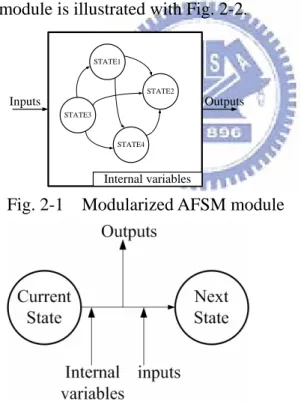
The chart of a modularized AFSM module is shown as Fig. 2-1. There are some states and

variables in a module. State transitions are determined according to transition functions

between states. These transition functions don’t only take current state and inputs as

parameters, but internal variables. The inputs come from other modularized AFSM modules;

The outputs of state transition are sent to other modularized AFSM modules. Transition

function of AFSM module is illustrated with Fig. 2-2.

STATE1 STATE4 STATE3 STATE2 Internal variables Inputs Outputs

Fig. 2-1 Modularized AFSM module

Fig. 2-2 Transition function of AFSM module

2.1.1 Why AFSM?

2.1.1.1 Simple Procedure for Decomposing and Combining

Rodney Brooks thinks that control mechanism of robot resembles animals: A RRCS can be

independent components composed of modularized AFSM modules interact with each other,

and therefore make up complete abilities for the RRCS. We’ll call these independent

components AFSM component .

Take human beings for example, the brain, hands, legs, and body are independent

components. Each component is composed of some parts. For instance, a hand is composed of

the skin, muscle, and bones. If we want to construct a human being by the concept of

AFSM-based RRCS, the hand will be counted in an AFSM component, and the skin, muscle,

and bones will be counted in modularized AFSM modules.

Because each AFSM module is a simple FSM, it can be handled by human being’s

capability. The simple procedure for decomposing and combining is one of the reasons why

we construct a RRCS with AFSM modules. After constructing some modularized AFSM

modules, these AFSM modules could connect with each other, and then they will become an

independent AFSM component. Finally, a complete RRCS is constructed with some AFSM

components. The structure of AFSM component is illustrated with Fig. 2-3.

Fig. 2-3 Independent AFSM component

2.1.1.2 Time Discretization

We had explained the purpose of discretization in 1.2, the first step of discretization

procedure is Time Discretization. In AFSM, time interval between current state and next state

which occurs at continuous time will be shifted to the closest discrete time point.

2.2 Roving Robot Collision Avoidance Experiment

After explaining the concept of AFSM, we will introduce the AFSM-based roving robot collision avoidance experiment [1] in detail.

The experiment had been simulated in [1]. In this work, we want to rebuild it, and check

the properties of the behaviors of the AFSM-based RRCS. The implementation of the

experiment will be discussed later in Chapter 5.

2.2.1 Experiment Overview

Fig. 2-4 The chart of the experiment

In the experiment, the robot is placed on a two-dimensional environment. The robot has

some sonar sensors for detecting the environment, and has a motor for generating force to

change its velocity. The motor can generate a force which has 8 kinds of directions, and make

the robot move towards 8 kinds of directions which are {U,D,L,R,LU,LD,RU,RD}. The robot

is controlled by AFSM-based RRCS, the RRCS monitors the information detected by sonar

sensors and then decides to issue what command to motor for changing the robot’s velocity.

Whenever the location of robot changes, sonar sensors will detect the environment. If there

are some obstacles within detection range of sonar sensors, the RRCS will decide new

obstacles; if there is no obstacle within detection range, the RRCS will let the robot wander

aimlessly around in the environment.

After constructing the AFSM-based RRCS for controlling the robot, we check some

properties of the behavior of the robot by OMocha.

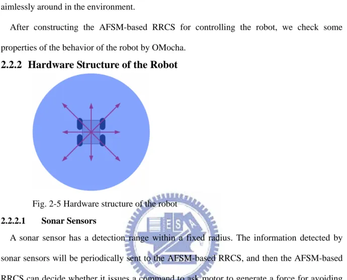
2.2.2 Hardware Structure of the Robot

Fig. 2-5 Hardware structure of the robot

2.2.2.1 Sonar Sensors

A sonar sensor has a detection range within a fixed radius. The information detected by

sonar sensors will be periodically sent to the AFSM-based RRCS, and then the AFSM-based

RRCS can decide whether it issues a command to ask motor to generate a force for avoiding

collision with obstacles or not.

2.2.2.2 Motor

The motor of robot continuously wait for a command sent by the AFSM-based RRCS.

There are two kinds of commands sent by the AFSM-based RRCS. The first kind of command

is “random force” command, the “random force” command asks the motor to generate a force

which has random degree and direction, and then the force will generate an acceleration

which makes the velocity of the robot to be changed. The second kind of command is

“assigned force” command, the “assigned force” command asks the motor to generate a force

which has assigned degree and direction. Finally, the “assigned force” command will change

the velocity of the robot as well as the “random force” command.

acceleration of robot has a range from 0 to Max_Force_Degree/M ; moreover, the degree of

robot’s velocity has a range from 0 to Max_Velocity_Degree. Therefore, if the degree of

robot’s velocity has reached Max_Veloctiy_Degree and then the motor will ignore the

“random force” or “assigned force” command which has the same direction as current

velocity.

2.2.3 Environment

Fig. 2-6 Environment of the experiment

The environment of the experiment is a two-dimensional space. Its shape is rectangle, and

has walls on four sides, and has some obstacles on four corners.

2.2.4 Expected Behaviors of the AFSM-based RRCS

The robot which is placed on a two-dimensional environment has two main abilities. The

two abilities are sensing obstacles by sonar sensor and moving around by motor. Based on the

two abilities provided by robot, the AFSM-based RRCS wants to make the robot achieve two

main behaviors：

A. Wander aimlessly keeping to Newton’s first and second laws of motion.

B. Make the robot avoid collision with obstacles in environment.

z

How to achieve the two behaviors

The first behavior can be achieved more easily. The AFSM-based RRCS can periodically

issue a command to ask motor to generate a directional force, and the direction and degree of

between force and acceleration is “A=F/M1”. Therefore, the force will generate acceleration

for the robot, and then the velocity of the robot will be changed. Finally, the robot will move

to a new location according to latest velocity.

If the motor generates a force whose degree equals to 0, the robot will keep its original

velocity keeping to Newton’s first laws of motion.

After achieving the first behavior, the robot can wander aimlessly, but it can’t avoid

collision with obstacles in environment. In order to achieve the second behavior—“avoid

collision with obstacles”, the AFSM-based RRCS must monitor the information of the

environment detected by sonar sensors. If there is an obstacle in detection range of sonar

sensors, the AFSM-based RRCS will pass a command to ask motor to generate a force which

has a reverse direction of the obstacle, ant then the force will generate a reverse acceleration,

finally the robot will gradually keep away from the obstacle. Therefore, the approach can

keep the robot to avoid collision with obstacles in environment, and can achieve the second

behavior.

2.2.5 Properties To Be Verified

The property we want to check by OMocha is：

Whether the robot will collide with obstacles or walls?

The robot has the two above-mentioned behaviors can wander aimlessly around the

environment and try to avoid collision with obstacles. However, the strategy determined by

the RRCS for avoiding collision doesn’t guarantee the robot doesn’t collide with obstacles. In

the strategy for avoiding collision, the relationship between “Distance away from the

obstacles” and “Reverse acceleration” is the most important part.

In order to make sure the behavior of the strategy is the same as our expected behavior, we

must describe the property with Temporal Logic and check whether the strategy really makes

the robot not to collide with obstacles. The checking procedure is completed by OMocha.

1

Chapter 3

Model Checking for AFSM-based RRCS,

Concepts

After introducing AFSM and roving robot collision avoidance experiment, we’ll explain

how to verify an AFSM-based RRCS by model checker. In this section, we will explain the

principle of model checking by the verification procedure of model checker, OMocha [4]. The

introduction for OMocha is in Section 3.2.

In Section 3.1.1, we will give two examples for explaining the verification procedure. In

the two examples, we will use the formal input language for OMocha. The formal input

language for OMocha is explained in detail in Section 3.3.

3.1 Verification Procedure

The concept of verification procedure is step by step to explore all reachable states from

initial state, and then check whether all explored reachable states which represent the

behaviors of programs satisfy the properties.

3.1.1 Two Examples of Verification Procedure

3.1.1.1 Simple Example

Take a simple AFSM-based system shown in Fig. 3-1 as an example. The AFSM-based

system is composed of two AFSM modules. The property we want to check is “AG

((STATE_A=A2 && A_B=false)||(STATE_A=A1 && A_B=true))”. It means

whether “((STATE_A=A2 && A_B=false)||(STATE_A=A1 && A_B=true))” is

always true from initial state to all reachable states.

The definition of initial state is the combination of all variables’ initial values of a system.

The initial state of the AFSM-based system is { STATE_A=A1 , A_B=false , STATE_B=B1 }.

described in programs, the sequential state transition of the AFSM-based system is listed as

Table 3-1. The next state of the initial state, which is also the 2nd state of the AFSM system is

{STATE_A=A2 , A_B=false , STATE_B=B1 }. Then the next state of the 2nd state, which is

also the 3rd state of the AFSM system is { STATE_A=A1 , A_B=true , STATE_B=B1 }.

OMocha will keep on exploring the next state of every state. Finally, OMocha will find out

that the 2nd to the 5th states are all possible reachable states from the initial state. Then the 6th

to the 9th states repeat the value of the 2th to the 5th state, and so on. The all possible states of

the system include the initial state and all possible reachable states from the initial state.

During the procedure of exploring all possible states of the system, OMocha detects the

behaviors of the programs violate the properties at initial state. Therefore, the behaviors of the

programs don’t satisfy the properties.

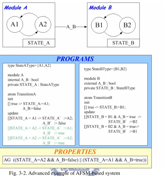
3.1.1.2 Advanced Example

After understanding the simple example of AFSM-based system, let us consider another

advanced example. In the advanced example, transition functions (update commands) are

allowed to include non-deterministic choices. As shown in Fig. 3-2, module A has a

non-deterministic choice as follow:

[]STATE_A = A2 -> STATE_A’:=A1; A_B’:= true []STATE_A = A2 -> STATE_A’:=A2; A_B’:= true

If the variables’ values of module A are { STATE_A=A2 , A_B=Don’t Care } in current

state, the variables’ values of module A may be { STATE_A=A1,A_B=true } or

{ STATE_A=A2,A_B=true } in next state. The sequential state transition of the advanced

AFSM example is listed as Table 3-2. The non-deterministic choices are provided to system

designer for simulating the random situation. In order to make the concept more clearly, we

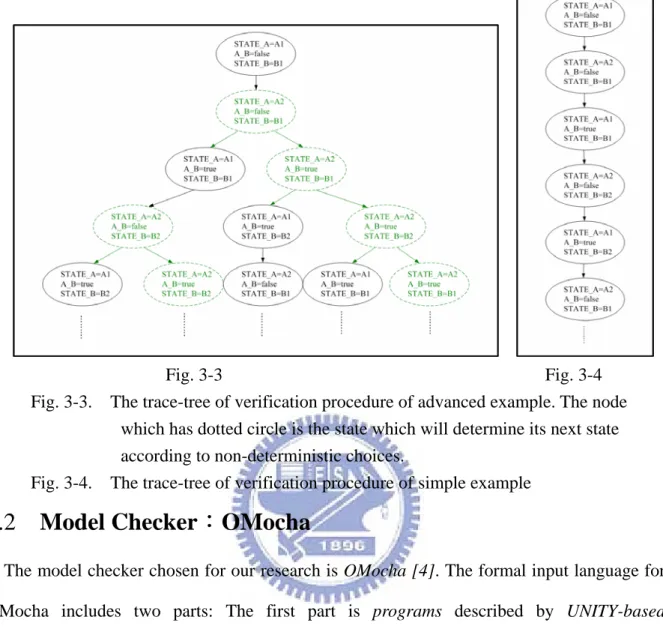
illustrate the trace-tree of verification procedure for the advanced example with Fig. 3-3.

according to the non-deterministic choices. Therefore, the trace-tree of verification procedure

for the advanced example is a multi-branch tree. However, the trace-tree of verification

procedure for the simple AFSM example is a single-branch tree as shown in Fig. 3-4.

Fig. 3-1. Simple example of AFSM-based system

variable state

STATE_A A_B STATE_B

1 A1 False B1 2 A2 False B1 3 A1 True B1 4 A2 False B2 5 A1 True B2 6 A2 False B1 ... ... ... ...

Table. 3-1. Sequential state transition of simple AFSM-based system

initial state

Fig. 3-2. Advanced example of AFSM-based system

variable state

STATE_A A_B STATE_B

1 A1 False B1 2 A2 False B1 3 A1 True B1 4 A2 False B2 5 A1 True B2 6 A2 False B1 7 A2 True B1 8 A1 True B2 9 A2 False B1 … … … …

Table. 3-2. Sequential state transitions of advanced AFSM-based system

initial state

Fig. 3-3 Fig. 3-4

Fig. 3-3. The trace-tree of verification procedure of advanced example. The node which has dotted circle is the state which will determine its next state according to non-deterministic choices.

Fig. 3-4. The trace-tree of verification procedure of simple example

3.2 Model Checker：OMocha

The model checker chosen for our research is OMocha [4]. The formal input language for

OMocha includes two parts: The first part is programs described by UNITY-based

specification language [2], and the second part is properties described by Temporal Logic [5].

After the formal input language is fed into OMocha, OMocha will check whether the

behaviors of the programs satisfy the properties. If the behaviors of the programs violate the

properties, OMocha will show one counterexample. Otherwise, it’ll show the behaviors of the

programs satisfy the properties.

. In Section 3.3, we’ll introduce the formal input language for OMocha.

3.3 Formal Input Language for OMocha

3.3.1 Programs Described by UNITY-based Specification Language

In OMocha, the programs are described by UNITY-based specification language. There are

two main reasons about why it uses UNITY to describe the programs as follows：

(1) UNITY could represent the relationship between current state and next state, what is

called transition function. Therefore, we could describe an AFSM-based RRCS by

UNITY.

(2) In order to operation in coordination with OMocha. In OMocha, the only data types can

be defined are cyclic integer and boolean, and the syntax and semantics of UNITY can

provide cyclic integer ( e.g., “A: bit[5]”, the range of cyclic integer A is from 0 to

31).

(B) Syntax and Semantics

There are two parts in programs:

(1)Module Description

In the first part of programs, we describe all AFSM modules in module description. For

describing a module, it includes two necessary parts: variables definition and atoms

definition.

Variables Definition

In variables definition, there are three kinds of variables can be defined: external, interface,

and private.

External variables---The input ports of AFSM module, they receive data from other AFSM modules’ interface variables.

Interface variables---The output ports of AFSM module, they send data to other AFSM modules’ external variables.

Private variables---The local variables of AFSM module, they don’t connect with other AFSM modules.

Three kinds of data types which can be defined for above three kinds of variables are

“cyclic integer”, “boolean” and “enum”.

Atoms Definition

In atoms definition, we describe the init action executed during initial round, and the

update action executed during each update round. The initial and update action are specified

by the keywords init and update. There are some init commands in initial action, and

there are some update commands in update action. An example for atoms definition is shown

as Fig. 3-6.

Fig. 3-6. Example for atoms definition

In each update round, every variable x has two values. The value of x at the beginning of

updated value. We use unprimed symbols, such as x, to refer to latched values, and primed

symbols, such as x’, to refer to the corresponding updated values.

The updated value of (N-1)th round is equal to the latched value of Nth round. The latched

value of x is also the current state of x, and the updated value of x is also the next state of x.

The relationship between latched value (current state) and updated value (next state) during

neighbor update rounds is shown as Fig. 3-7.

Fig. 3-7. The relationship between latched value and updated value during neighbor

update rounds.

Let us look the example shown in Fig. 3-6, the updated value of STATE and A are init and 1

at initial round. According to the update command in update action, if the latched value of

STATE and A are init and 1, the updated value of them will be set to start and 2. Therefore,

the updated values of STATE and A are start and 2 at 1st update round. Update commands

which determine the relationship between latched values and updated values, can regard as

transition functions which determine relationship between current state and next state.

(2) Module Connection

After all AFSM modules are described in module description, we need to describe the

connection relationship between these AFSM modules. An interface variable can connect with

some external variables of other AFSM modules which have the same name as the interface

variable. An external variable can only connect with an interface variable of another AFSM

3.3.2 Properties Described by Temporal Logic

(A) Introduction

In OMocha, the method chosen to describe the properties of an AFSM-based RRCS is

Temporal Logic.

Temporal Logic is used to represent the properties of state transitions of a system over time

domain. For instance, we want to check whether variable A is always less than 10 during all

possible states. In this case, the representation of Temporal Logic is “AG A<10”, the meaning

of ”AG” is “always true” during all possible states from initial state. After describing the

programs of an AFSM-based RRCS by UNITY, we can describe the properties of the

AFSM-based RRCS by Temporal Logic, and the properties are what we want to check by

OMocha. When OMocha receives the formal input language including programs and

properties, it can check whether the behaviors of the programs satisfy the properties.

(B) Syntax and Semantics

Every property of a system is described by Temporal Logic. A Temporal Logic formula

consists of the propositional logic formula and temporal connectives： The propositional

logic formulas are expressions which consist of logical operators and the variables of the

system. The temporal connectives are expressions to indicate the subset of future states of the

system.

The temporal connectives are pairs of symbols：

The first member of the pair is one of

A - meaning on all paths from the “current” state, read as “inevitably”

E - meaning on at least one path from the ”current” state, read as “possibly”

The second member of the pair is one of

G - meaning all future states, read as “globally”

F - meaning some future state

U - meaning until

Take “mutual exclusion” as example. Suppose we are talking about two processes P1, P2

that share data. The protocol allows only one process to be in its critical section at any time.

If we want to describe the “mutual exclusion” property by Temporal Logic, the Temporal

Logic formula will be described as follow：

AG !( Critical[P1] & Critical[P2] )

The propositional logic formula !( Critical[P1] & Critical[P2])

The temporal connectives AG

This Temporal Logic formula is true iff Critical[P1] and Critical[P2] won’t be

Chapter 4

Model Checking for AFSM-based RRCS,

Approaches

In this Chapter, we present three approaches to lower the difficulty of formal verification

for the experiment. After using the three approaches to reduce the number of states of the

RRCS and environment, formal verification can become applicable for the experiment.

4.1 State Space Discretization

A system described on the continuous domain can’t be verified by OMocha, because the

number of all possible states is infinite. Before constructing an AFSM-based RRCS we must

transform the system and environment from continuous domain to discrete domain. Otherwise,

OMocha can’t handle it.

In discretization procedure, there are two parts. (1) Time Discretization, and (2) Space

Discretization. Time Discretization has been explained in Section 2.1.1.2, therefore we will

only explain Space Discretization in this section. We will give two examples to illustrate the

relationship between continuous space and discrete space below.

Take a simple MAP as first example, the continuous MAP whose size is 2*2 m2 is

transformed into a discrete MAP. In x-axis and y-axis, the continuous domain is partitioned

into 21 points separately (x-axis:0.1.2….20, y-axis:0.1.2….20). Therefore, the distance

between two neighbor points is 0.1m, and the size of the discrete MAP is 21*21. The

Fig. 4-1. (a) continuous MAP (b) discrete MAP

Then, we give another example. In Section 2.2.5, we have mentioned that in the strategy for

avoiding collision, the relationship between “Distance away from the obstacles” and “Reverse

acceleration” is the most important part. In Fig. 4-2, we illustrate the relationship between

continuous domain and discrete domain in this example.

Fig. 4-2 (a) continuous domain (b) discrete domain

In Fig. 4-2, “Reverse acceleration” is approximately linear inverse proportion to “Distance

away from the obstacles” on continuous domain, the curve presents the relationship between

the two parameters. The number of all possible mapping relations of them is infinite, the

mapping set includes { (0, 5)..(0.5,4.5)..(3.5,1.5)..(5,0) }. After transformation, the mapping

set has only fix points on discrete domain, they are { (0,5) . (1,4) . (2,3) . (3,2) . (4,1) . (5,0) }.

After discretization procedure, the complexity of a system will be simplified to the degree

4.2 External Function for Computation/State Hiding

In order to improve the capabilities which the UNITY-based programs can support, and

reduce the number of states of a system. OMocha provides the external function for system

designer. The two main advantages are listed below：

4.2.1

Computation Hiding

The semantics and syntax of UNITY are very basic and aren’t as powerful as high-level

language. For this reason, it’ll be very hard to build complicated programs of a system by

UNITY.

In order to improve the capabilities which the UNITY-based programs can support,

OMocha provides the external function for system designer. The external function is

described by C language. The UNITY which includes external function is called advanced

UNITY.

In original UNITY, the semantics and syntax can only provide basic capabilities, these

basic capabilities include：

Value assignment

Basic logic operations: and/or/not/invert

Basic arithmetic operations: addition/subtraction

Basic comparison operators: > <

Non-nested if-then-else structure

……etc

In advanced UNITY, we can pass variables into external functions, and then receive the

return value of external function by variables which defined in UNITY.

There are two examples for explaining computation hiding through external function. The

Example 1

A part of programs described with original UNITY

The same part described with advanced UNITY

Example 2

A part of programs described with original UNITY

4.2.2

State Hiding：Reducing the Number of All Reachable States of a

System

How complicated a system can be verified by OMocha depends on the number of all

reachable states. Once the number of all reachable states of a system is greater than the

limitation of OMocha’s capability, the “out of memory” problem will occur during checking

procedure. Therefore, we have to carefully control the complexity of a system so that the

resource (memory, CPU speed...etc) of OMocha can handle the checking procedure.

The number of all reachable states of a system depends on the all possible combination of

all variables which are defined in UNITY-based programs. If we can move out some variables

which are defined in UNITY-based programs, and encapsulate them into external function,

the number of all reachable states will reduce.

But, what kinds of variables can be encapsulated into external function ？ During

verification procedure, there are some system variables which are irrelevant to behavior

verification. For example, in the experiment explained in Chapter 2, OMocha only needs to

know the velocity and location of the robot whereas it doesn’t need to know the computation

of detecting environment, and determining the degree of acceleration. The variables for

detecting environment and determining the degree of acceleration can be exported to external

function.

An example of the encapsulation procedure of external function is shown as Fig. 4-3. In Fig.

4-3, the system is composed of four AFSM modules. There is one interface variable in each

module, so the total number of the variables in the system is four. According to encapsulation

principle, if a module doesn’t include some nondeterministic update commands, it can be

encapsulated into a external module. Take the system as a example, the module B, module C

and module D can be encapsulated into a external module which invokes a external function

to handle all update commands of them, the encapsulation procedure shown as Fig 4-3(c). The

nondeterministic update command. After encapsulation procedure, the system reduces the

number of modules from 4 to 2, and reduces the number of variables from 4 to 2. The two

interface variables Bout,Cout are encapsulated into the external function “Ext_fun”, so model

checker doesn’t need to consider them. In some cases, reducing the number of variables by

encapsulation procedure can obviously lower the number of all reachable states of the system

Fig. 4-3. Encapsulation procedure

(a) A system is composed of four AFSM modules

(b) The module B, module C and module D can be encapsulated into a external module

(c) The three modules will be integrated into one external module, the UNITY-based programs of the external module and C code of external function Ext_fun() are shown in the figure.

4.3 Elimination of Unnecessary Checking Cases

The concept of verification procedure is step by step to explore all reachable states from

initial state. Therefore this is a kind of method of exhaustion. However, according to the

properties we want to check by OMocha, we can eliminate some unnecessary checking cases,

because this part of checking cases will never violate the properties. Take the experiment

explained in Chapter 2 as example. The robot will never collide with obstacles while it

wanders aimlessly in the range which has no obstacles. Therefore, OMocha can eliminate the

Chapter 5

Implementation of Roving Robot Collision

Avoidance Experiment

In this Chapter, we will present how to construct the AFSM-based RRCS and environment

in the experiment with UNITY, and explain the AFSM-based RRCS in detail.

We have explained the chart of an AFSM module in Section 2.1, and explained how to

describe the programs of an AFSM module has explained in Section 3.3.1. These two sections

are the most important foundations for this section.

In Section 5.1, we will show the full structure of the experiment, and then briefly introduce

these AFSM modules in the experiment. In Section 5.2, we introduce every AFSM module in

detail, and how these AFMS modules connect with other modules and work in coordination.

In Section 5.3, we explain the “No_Collision” property described by Temporal Logic. The

checking results of the experiment are explained in Chapter 6.

5.1 Full Structure of the Experiment

Fig. 5-1 Full structure of the experiment

composed of 6 AFSM modules, and environment is composed of 1 AFSM module. These

modules are listed in Table 5-1：

Module name

Module figure

Functionality

MAP

z Set the position of obstacles and walls into

MAP_walls and MAP_obstacles at initial round.

z Provide the map of environment to other modules through interface variable

SONAR

z In each round, SONAR reads Location_updated from MOTOR module, and then SONAR detects the

environment and produces the robot centered map of

obstacles and walls

z Provide the robot centered map stored in

SMAP_obstacle to FORCE_ACCELERATION

and RANDOM_ACCELERATION modules.

FORCE_ ACCELERATION

z In each round, FORCE_ACCELERATION awaits robot centered map of obstacles from SONAR

module, and then compute

Force_Acceleration for

RESULT_ACCELERATION module

RANDOM_ ACCELERATION

z In each round, If there is no any obstacle in detection range(the updated value of SMAP_obstacle is

{(0,0),LU} ), RANDOM_ACCELERATION module

produces a random Random_Acceleration for

RESULT_ ACCELERATION

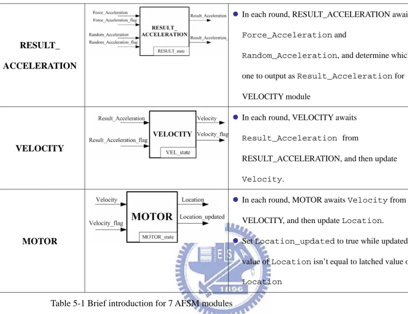
z In each round, RESULT_ACCELERATION awaits Force_Acceleration and

Random_Acceleration, and determine which

one to output as Result_Acceleration for

VELOCITY module

VELOCITY

z In each round, VELOCITY awaits Result_Acceleration from

RESULT_ACCELERATION, and then update

Velocity.

MOTOR

z In each round, MOTOR awaits Velocity from VELOCITY, and then update Location.

z Set Location_updated to true while updated value of Location isn’t equal to latched value of Location

Table 5-1 Brief introduction for 7 AFSM modules

5.2 Introduction for each AFSM Module in detail

1. MAP：

Fig. 5-2 MAP module

z Set the position of obstacles and walls into MAP_walls and MAP_obstacles at initial round.

z Provide the map of environment to other modules through interface variable

The MAP module is for simulating the environment. In MAP module, we set the position of

obstacles and walls in environment map at initial round. The representation of obstacle or wall

is { position , direction }. The position is represented by (position of X-axis ,position of

Y-axis), and the direction includes four kinds of directions, which are

{LU(left-up),LD(left-down),RU(right-up),RD(right-down)}. In Fig. 5-3, we list some examples to illustrate the usage of the representation.

Example of wall

Representation { (8,0),LU/LD } { (34,0),RU/RD } { (0,8),LD/RD } { (0,34),LU/RU }

Example of obstacle

Representation { (12,30) , LU } { (12,12) , LD } { (30,12) , RD } { (30,30) , RU } Fig. 5-3 Some examples for the representation of MAP_obstacle/MAP_wall

Take the MAP1.0 shown in Fig. 5-4 as example of environment. The position of walls are

{ (8,0)} , LU } , { (38,0), RU } , { (0,8) , LD } , { (0,38) , RU }, and the position of obstacles

are { (12,12) ,LD },{ (34,12) , RD },{ (12,34) , LU },{ (34,34) , RU }. According to the

representation, we can set the values of MAP_obstacles and MAP_walls. The interface

variables MAP_obstacles and MAP_walls will be sent to SONAR module.

variables MAP_obstacle1-4 and MAP_wall1-4 will connect to SONAR module for

informing the map of environment.

The figure and features of MAP1.0 is shown as Fig 5-4. The MAP 1.0 is very simple. It is a

two-dimensional square whose size is 30*30, and the obstacles can only expand from 4

corners. Because there is only “unsigned ranged integer” data type in OMocha, we reserve the

boundary buffer area around the environment. The reason is in order to avoid the appearance

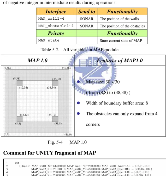
of negative integer in intermediate results during operations.

Interface

Send to

Functionality

MAP_wall1~4 _{SONAR The position of the walls} MAP_obstacle1~4 _{SONAR The position of the obstacles}

Private

Functionality

MAP_state Store current state of MAP

Table 5-2 All variables in MAP module

MAP 1.0

Features of MAP1.0

z Map size: 30 x 30 ( from (8,8) to (38,38) )

z Width of boundary buffer area: 8

z The obstacles can only expand from 4 corners

Fig. 5-4 MAP 1.0

Comment for UNITY fragment of MAP

In the UNITY fragment of MAP shown as Fig. 5-5, we set position of walls and obstacles

into MAP_obstacles and MAP_walls.

Line 1： The initial action of atoms is specified by the keywords init.

Line 2-9： Set the value of MAP_obstacles and MAP_walls.

Line 4： The position of MAP_wall3 is (0, 8), and the direction is LD.

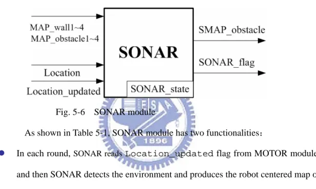
2. SONAR：

Fig. 5-6 SONAR module

As shown in Table 5-1, SONAR module has two functionalities：

z In each round, SONAR reads Location_updated flag from MOTOR module, and then SONAR detects the environment and produces the robot centered map of

obstacles and walls

z Provide the robot centered map stored in SMAP_obstacle to

FORCE_ACCELERATION and RANDOM_ACCELERATION modules.

SONAR module is the module to simulate the behavior of sonar sensor on the robot. It receives the map of environment from MAP module and location of robot from MOTOR module. After receiving above external variables from MAP and MOTOR module, SONAR module will produce a robot centered map of obstacles and walls according to the detection range of sonar sensor. The detection range of sonar sensor is a robot centered range whose size is 16x16, and for every quadrant the size is 8x8. The figure of detection range is shown as Fig. 5-7.

Fig. 5-7 Detection range

The information of the robot centered map of obstacles and walls is stored in the interface

variable SMAP_obstacle, and the SMAP_obstacle will be sent to

FORCE_ACCELERATION and RANDOM_ACCELERATION modules.

The representation of SMAP_obstacle is { distance ,direction }, the distance in the

representation are represented with the distance away from the obstacle or wall for X-axis and

Y-axis separately. In Fig. 5-8, we list some examples to illustrate the usage of the

representation for SMAP_obstacle.

Example

representation {(4,5),RU} {(2,3),LD} {(0,5),LD/RD} {(6,0),LU/LD}

Fig. 5-8. Some examples for the representation of SMAP_obstacle

The introduction for all variables in SONAR module is shown in Table 5-3. In each round,

SONAR module reads MAP_obstacle1-4 and MAP_wall1-4 from MAP, and reads Example

Location and Location_updated from MOTOR, and then it updates the updated

value of SMAP_obstacle and SONAR_flag. The interface SMAP_obstacle and

SONAR_flag connect to FORCE_ACCELERATION and RANDOM_ACCELERATION

modules for informing the robot centered map of obstacles and walls. The private variable

SONAR_state is for storing the state of SONAR module.

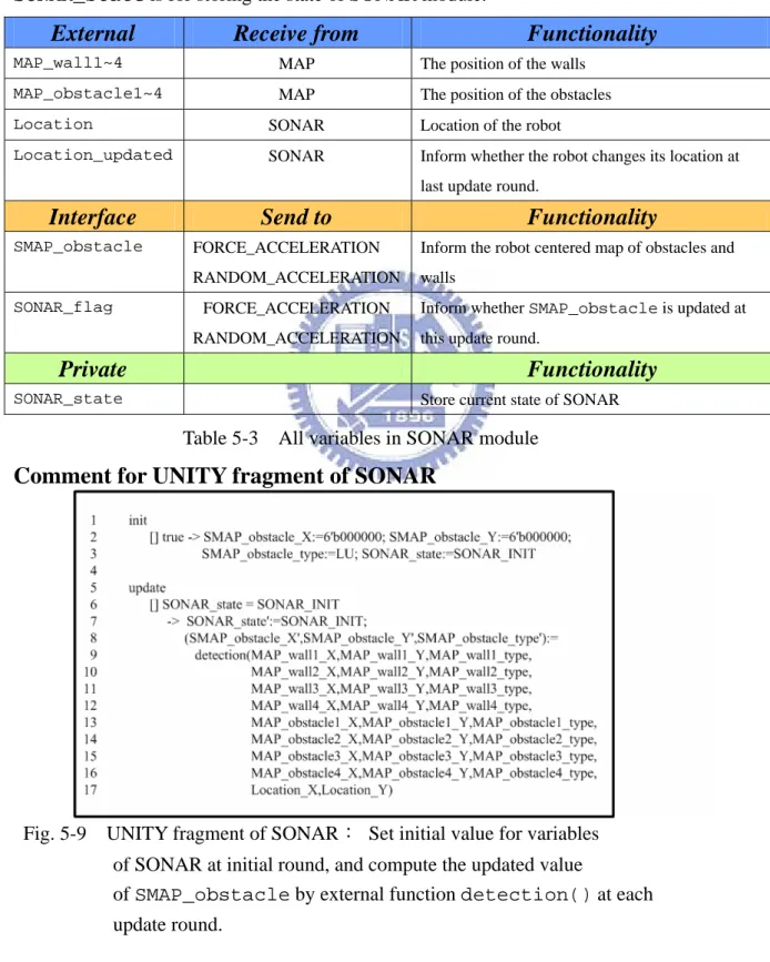
External

Receive from

Functionality

MAP_wall1~4 _{MAP The position of the walls} MAP_obstacle1~4 _{MAP The position of the obstacles} Location SONAR Location of the robot

Location_updated SONAR Inform whether the robot changes its location at last update round.

Interface

Send to

Functionality

SMAP_obstacle _{FORCE_ACCELERATION} RANDOM_ACCELERATION

Inform the robot centered map of obstacles and walls

SONAR_flag FORCE_ACCELERATION RANDOM_ACCELERATION

Inform whether SMAP_obstacle is updated at this update round.

Private

Functionality

SONAR_state _{Store current state of SONAR}

Table 5-3 All variables in SONAR module

Comment for UNITY fragment of SONAR

Fig. 5-9 UNITY fragment of SONAR： Set initial value for variables of SONAR at initial round, and compute the updated value

of SMAP_obstacle by external function detection() at each update round.

In the UNITY fragment of SONAR shown as Fig. 5-9, we set initial value for variables of SONAR at initial round, and compute the updated value of SMAP_obstacle by external function detection() at each update round. Because the strategy of computing

SMAP_obstacle is too complicated to write by UNITY code, we implement the strategy by external function detection().

Line 2-3： Set initial value for SMAP_obstacle

Line 5： The update action of atoms is specified by the keywords update.

Line 6： In this update rule, if latched value of SONAR_state is SONAR_INIT, Line7-17

will be executed.

Line 7： The updated value of SONAR_state is updated to SONAR_INIT

Line 8-17： The updated value of SMAP_obstacle is computed by external function

detection()

Fig. 5-10 Fragment of external function detection()

Line 1-9： detection() receives MAP_walls,MAP_obstacles and Location as parameters

Line 11： Declare local variable SMAP_obstacle.

Line 15-19： Check whether MAP_wall1 (direction:LU/RU) is in the detection range. If it’s true, SMAP_obstacle_Y will be set to “MAP_wall1_Y - Location_Y” and SMAP_obstacle_type will be set to “LU”.

Line 24： Return the value of local variable SMAP_obstacle. The return value will be assigned to interface variable SMAP_obstacle in SONAR module.

Example

If ( MAP_wall1_X=0, MAP_wall1_Y=8, MAP_wall1_type=LU,

Location_X=18, Location_Y=6)

Then (SMAP_obstacle_X=0, SMAP_obstacle_Y=2, SMAP_obstacle_type=LU)

3. FORCE_ACCELERATION：

Fig. 5-11 FORCE_ACCELERATION module

As shown in Table 5-1, FORCE_ACCELERATION module has one functionality：

z In each round, FORCE_ACCELERATION awaits robot centered map of obstacles from SONAR module, and compute the Force_Acceleration for

RESULT_ACCELERATION module

In FORCE_ACCELERATION module, it receives SMAP_obstacle from SONAR

module, and then produces the “reverse acceleration” according to the strategy for avoiding

colliding with obstacles, the result of “reverse acceleration” is stored in interface variable

Force_Acceleration. The relationship between“distance of X-axis away from the

obstacle in SMAP_obstacle” and “X-axis component of reverse acceleration degree in

Force_Acceleration” is shown as Table 5-4.

Distance of X-axis away from

the obstacle in SMAP_obstacle 0 1 2 3 4 5 6 7 X-axis component of reverse acceleration

Degree in Force_Acceleration 0 2 2 2 1 1 1 1

Table 5-4 The relationship between “Distance of X-axis away from the obstacle in SMAP_obstacle” and “X-axis component of reverse acceleration degree in Force_Acceleration”. Take X-axis for instance, the situation of Y-axis is equivalent to X-axis

The representation of Force_Acceleration is { A-degree ,direction }, the A-degree is

represented by (degree of X-axis component,degree of Y-axis component), and the range of

A-degree is from 0 to 2; the direction is reverse to the direction of SMAP_obstacle. We list some examples to illustrate the relationship between SMAP_obstacle and

Force_Acceleration in Fig. 5-12.

Example

SMAP_obstacle {(4,5),RU} {(2,3),LD} {(0,5),LD/RD} {(6,0),LU/LD}

Force_Acceleration {(1,1),LD} {(2,2),RU} {(0,1),RU/LU} {(1,0),RD/RU}

Example

SMAP_obstacle {(0,5),RU} {(6,5),LD} {(4,4),RU} {(4,5),LD}

Force_Acceleration {(0,1),LD} {(1,1),RU} {(1,1),LD} {(1,1),RU} Fig. 5-12 Some examples of the relationship between SMAP_obstacle and

Force_Acceleration

The introduction for all variables in FORCE_ACCELERATION module is shown as

Table 5-5. FORCE_ACCELERATION awaits SMAP_obstacle from SONAR module, and

then updates the updated value of Force_Acceleration. The interface

Force_Acceleration and Force_Acceleration_flag connect to

RESULT_ACCELERATION module for informing force acceleration.

External

Receive from

Functionality

SMAP_obstacle _{SONAR The robot centered map of obstacles and} walls

updated at this update round

Interface

Send to

Functionality

Force_Acceleration RESULT_ACCELERATION Inform the force acceleration for RESULT_ACCELERATION.

Force_Acceleration_flag RESULT_ACCELERATION Inform whether the updated value of degree of Force_Acceleration is non-zero at this update round. It is set true while the updated value of degree of

Force_Acceleration is not (0,0).

Private

Functionality

FORCE_state Store current state of

FORCE_ACCELERATION

Table 5-5 All variables in FORCE_ACCLERATION module

Comment for UNITY fragment of FORCE_ACCELERATION

Fig. 5-13 UNITY fragment of FORCE_ACCELERATION：

Set initial value for variables of FORCE_ACCELERATION at initial round,

and compute the updated value of Force_Acceleration by external

function SMAP_to_FORCE() at each update round.

Line 2-3：Set initial value for FORCE_ACCELERATION

Line 6-7：The updated value of Force_Acceleration is computed by

Fig. 5-14 Fragment of external function SMAP_to_FORCE()

Line 1： SMAP_to_FORCE() receives SONAR_flag and SMAP_obstacle as

parameters

Line 3： Declare local variable Force_Acceleration.

Line 8-18： If SONAR_flag is true, we set the value of Force_Acceleration_X

according to relationship shown in Table 5-4.

Line 25-31： If SONAR_flag is true, we set the value of Force_Acceleration_type

according to relationship shown in Fig. 5-12.

Line 35：Return the value of local variable Force_Acceleration. The return

value will be assigned to interface variable Force_Acceleration

4. RANDOM_ACCELERATION：

Fig. 5-15 RANDOM_ACCELERATION module

As shown in Table 5-1, RANDOM_ACCELERATION module has one functionality：

z In each round, if there is no any obstacle in detection range (the updated value of SMAP_obstacle is { (0,0) , LU) ), RANDOM_ACCELERATION module produces a

random Random_Acceleration for RESULT_ACCELERATION module.

In RANDOM_ACCELERATION module, it awaits SMAP_obstacle from SONAR

module. If there is no obstacle in detection range (the updated value of

SMAP_obstacle is {(0,0) , LU} ), RANDOM_ACCELERATION module will produce

a random acceleration for the robot. The robot can wander aimlessly by changing its

velocity according to the random acceleration. The random acceleration which produced

by RANDOM_ACCELERATION is stored in interface variable

Random_Acceleration, and then Random_Acceleration will be sent to

RESULT_ACCELERATION module.

The representation of Random_Acceleration is {A-degree ,direction }, the

A-degree is represented by (degree of X-axis component, degree of Y-axis component), and the range of A-degree is from 0 to 2; the direction is one of { LU,LD,RU,RD }. We

list some examples of the relationship between SMAP_obstacle and

Random_Acceleration in Fig. 5-16.

Table 5-6. In each round, RANDOM_ACCELERATION awaits SMAP_obstacle from

SONAR module, and updates the updated value of Random_Acceleration and

Random_Acceleration_flag. The interface Random_Acceleration and

Random_Acceleration_flag connect to RESULT_ACCELERATION modules for

informing the random acceleration.

Example

SMAP_obstacle {(0,0),LU} {(0,0),LU} {(0,0),LU} Not {(0,0),LU}

Random_Acceleration {(2,2),RU} {(2,1),RD} {(1,2),LD} {(0,0),LU} Fig. 5-16 Some examples of the relationship between SMAP_obstacle and

Random_Acceleration

External

Receive from

Functionality

SMAP_obstacle _{SONAR The robot centered map of obstacles and walls} SMAP_obstacle_flag _SONAR Inform whether SMAP_obstacle is updated

at this update round

Interface

Send to

Functionality

Random_Acceleration RESULT_ACCELERATION Inform the random acceleration for RESULT_ACCELERATION

Random_Acceleration_flag RESULT_ACCELERATION Inform whether the updated value of degree of Random_Acceleration is non-zero at this update round. It is set true while the updated value of the degree of

Random_Acceleration is not (0,0).

Private

Functionality

RANDOM_state Store current state of

RANDOM_ACCELERATION

Comment for UNITY fragment of RANDOM_ACCELERATION

Fig. 5-17 UNITY fragment of RANDOM_ACCELERATION：

Set the initial value for variables of RANDOM_ACCELERATION at initial round, and update the updated value of Random_Acceleration_X at each update round.

Line 2： Set initial value for RANDOM_ACCELERATION

Line 4-6 ： If (SMAP_obstacle_X,SMAP_obstacle_Y) is (0,0), the value of

Random_Acceleration_X will randomly be set to one of {0,1,2}

Line 7：If one of SMAP_obstacle_X and SMAP_obstacle_Y is not 0, the value of

Random_Acceleration_X will be set to 0.

5. RESULT_ACCELERATION：

Fig. 5-18 RESULT_ACCELERATION module

As shown in Table 5-1, RESULT_ACCELERATION module has one functionality：

z In each round, RESULT_ACCELERATION awaits Force_Acceleration and Random_Acceleration, and then determine which one to output as

Result_Acceleration for VELOCITY module

Random_Acceleration, and then determines which one to output as

Result_Accleration for VELOCITY module. The strategy for making the decision is

listed below:

A. Force_Acceleration_flag==true&&Random_Acceleration_flag==false/

trueÆ Result_Acceleration = Force_Acceleration

B. Force_Acceleration_flag==false&&Random_Acceleration_flag==true

Æ Result_Acceleration = Random_Acceleration

C. Force_Acceleration_flag==false&&Random_Acceleration_flag==false

ÆResult_Acceleration = { (0,0) , LU }

The strategy includes three conditions：

A. If Force_Acceleration_flag is true, Force_Acceleration will be stored in

Result_Acceleration.

B. If Force_Acceleration_flag is false and Random_Acceleration_flag is

true, Random_Acceleration will be stored in Result_Acceleration.

C. If Force_Acceleration_flag and Random_Acceleration_flag are both

false, Result_Acceleration will be set to { (0,0) , LU }.

The strategy will make the robot avoid collision while there are some obstacles in detection

range ,and wander aimlessly while there is no obstacle in detection range.

The introduction for all variables in RESULT_ACCELERATION module is shown in

Table 5-7. RESULT_ACCELERATION awaits Force_Acceleration from FORCE_-

ACCELERATION and Random_Acceleration from RANDOM_ACCELERATION,

and then updates the updated value of Result_Acceleration. The interface

Result_Acceleration and Result_Acceleration_flag connect to VELOCITY