國 立 交 通 大 學
電機與控制工程學系
碩 士 論 文
以車道線偵測為基礎之
駕駛人昏睡警示安全系統
A Lane-Based Drowsiness Estimation System for
Safety Driving
研 究 生:林立倬
指導教授:林進燈 博士
中華民國 九十六 年 七 月
以車道線偵測為基礎之駕駛人昏睡警示安全系統
A LANE-BASED DROWSINESS ESTIMATION SYSTEM
FOR SAFETY DRIVING
研 究 生:林立倬 Student:Li-Juo Lin
指導教授:林進燈 博士
Advisor:Dr. Chin-Teng Lin
國立交通大學
電機與控制工程學系
碩士論文
A Thesis
Submitted to Department of Electrical and Control Engineering
College of Engineering and Computer Science
National Chiao Tung University
in Partial Fulfillment of the Requirements
for the Degree of Master
in
Electrical and Control Engineering
July 2007
Hsinchu, Taiwan, Republic of China
以車道線偵測為基礎之
駕駛人昏睡警示安全系統
學生:林立倬
指導教授:林進燈 博士
國立交通大學電機與控制工程研究所
Chinese Abstract中文摘要
近年來,由於車輛數目的快速成長,造成交通事故問題日益嚴重。在台灣, 每年有超過兩千五百人在車禍中喪生。而根據交通部的資料,過去的四年中,每 年至少有八萬多件的車禍事故發生。這種情況下促成智慧型運輸系統(Intelligent transportation system, ITS)相關研究的發展越來越受到關注。而大部分車禍發生的 原因主要由於駕駛人本身的分心、不注意車況、疲勞駕駛等不適當駕駛行為所引 起。因此,為了能盡量避免駕駛者身處於此危險狀態,我們針對車輛後照鏡旁的 側邊影像資訊,開發一套以智慧型視覺技術為基礎的車道偵測及偏移系統,以確 保駕駛人行駛的安全性。 在車道線偵測部分,為了提高車輛側邊的視角範圍,我們將一支魚眼 (Fish-Eye)攝影機架設在後照鏡下方,並利用車體資訊在連續影像中固定的特 性,自動選取路面範圍,而不需要事先得知攝影機架設的相關資訊。為了可適用 於全天候的光線變化條件,我們同時處理空間及時間軸上的影像資訊,使此系統 在白天及夜間人眼可視車道範圍內,都能獲得清晰的車道邊界資訊。另外本論文 提出一套分段直線搜尋模組來連結車道線的軌跡,以提升整個搜尋速度,並克服 魚眼鏡頭失真的問題。 在車道偏移判斷的部分,本論文利用先前偵測的車道側向位置,及TLC(Time to Lane Crossing)的瞬時資訊,規劃車道偏移警示的觸發條件。另外建立一個可以即時更新的車道線位移穩定區間,來模擬駕駛人在直線道路行駛時和車道線 保持習慣性距離的特性。最後我們和交通大學腦科學中心(Brain Research Center, NCTU)合作,取得其在虛擬實境動態模擬駕駛系統的環境下,針對駕駛人昏睡 狀態預測的相關數據,套用在實際駕駛的影像內容中,使本系統除了估測車道 偏移的外在因素外,也可針對駕駛人本身的精神狀況作更進一步的分析,以提 升本系統的安全性及可靠性。 本論文發展的車道偵測輔助系統在 1.83GHz 的 PC 平台上平均可達超過 15fps 的執行結果。測試影像內容為在高速公路的實際駕駛環境,並在白天及夜 間範圍內都維持穩定的偵測結果。
A Lane-Based Drowsiness Estimation System
for Safety Driving
Student: Li-Juo Lin
Advisor: Dr. Chin-Teng Lin
Department of Electrical and Control Engineering
National Chiao Tung University
English Abstract
Abstract
As the high growth of population of vehicles, the traffic accidents are becoming more and more serious in recent years. In Taiwan, more than two thousand and five hundred people are died in traffic accidents every year. For each of last four yours, the number of traffic accidents is at least eighty thousand according the statistics of the Ministry of Transportation and Communications (MOTC, R.O.C.). In this situation, a lot of researches about the intelligent transportation system (ITS) have been paid more and more attention to the researches of related fields. Most occurrence of the car accidents results from the distraction, inattention for the adjacent cars, and driving fatigue of the driver. As a result, to avoid the driver being in danger as much as possible, an intelligent vision-based system focused on image contents of lateral-view camera setting under the rear-view mirror on vehicle is developed about lane detection and lane departure warning in this study.
In this thesis of lane detection, a fish-eye camera is located on the vicinity of the rear-view mirror to increase the range of lateral-view angle. Furthermore, we make use of the invariant of image for car body fixed in consecutive image sequences to extract the ROI (region of interest) containing the road surface without realizing the
intrinsic and extrinsic parameters of camera in advance. To make this algorithm suitable for various light conditions all day, the information of image in spatial and temporal domain must be simultaneously processed so that the lane boundary keeps distinct whether people have seen in the day or night environment. On the other hand, a piece-wise line searching model proposed in this paper is to connect the trajectory of lane and to reduce the computation load and to overcome the fish-eye lens distortion. In the thesis of lane departure warning, the instantaneous information of the lateral position from the result of lane detection and the TLC (time to lane crossing) can be regarded as the warning triggers for the alarms of lane departure. Then, a stable-driving region with real-time update mechanism is constructed to simulate the straight-road driving habit of different drivers which get used to keep approximately the same distance between the vehicle and lane markers. Eventually, by cooperated with the BRC (Brain Research Center, NCTU), we utilize the statistics about drowsiness estimation of the drivers in Virtual-Reality (VR) dynamic driving simulator to implement in the video contents for realistic driving. Therefore, this mechanism can be not only estimated the external factors such as departure of lane boundary but the internal ones such as the conscious analysis of the driver with higher reliability and safety.
The lane detection and departure warning system proposed in this paper has been successfully evaluated on the PC platform of 1.83-GHz CPU with the average frame-rate is up to 15fps. Moreover, this algorithm can be maintained stable results whether in the day or night environment of the realistic driving on highway.
Chinese Acknowledgements
致 謝
本論文的如期完成,要感謝的人實在太多了。尤其是這兩年的研究生 涯,無論是學術上還是生活上的幫助,心中總是對這段時間中曾經在旁陪 伴及鼓勵我的人們,保持著滿滿的感激及謝意。 首先要感謝指導教授 林進燈博士的悉心指導,在學術上引導著我走 向正確的研究方向。老師同時也給予我很大的空間來盡情發揮想像力及創 造力,讓我學習到如何面對及解決問題的正確態度和方法。另外也要感謝 傅立成教授、郭耀煌教授不遠千里的來擔任我的口試委員,你們的建議及 指教,使本論文的內容架構更為完整。 其次,感謝超視覺實驗室的蒲鶴章、劉得正及范剛維學長,在研究理 論及實務上給予我相當多的幫助與建議,讓我獲益良多。也感謝 Vision Group 的博士班學長姊們,及同學亞書、育宏、訓緯及肇廷的相互砥礪, 及所有學弟妹們在研究過程中給我的鼓勵與協助。另外感謝腦科學中心鄭 仲良同學,提供我很多實驗上的想法及數據參考。以及室友佳華、嘉川、 存智在這段時間和我共同度過許許多多難忘的回憶,謝謝你們。 最後要感謝一路走來默默支持我的家人們:我的父母、姐姐、以及哥 哥給予我精神及物質上的一切支援,也感謝其他親人對我不斷的關心與鼓 勵。特別感謝我的良師兼親友─我的姐夫簡韶逸先生兩年來在研究上給予 我許多正確及珍貴的建議。你們的關心及支持,才是我保持研究動力的精 神來源。 謹以本論文獻給我的家人及所有關心我的師長與朋友們。Contents
Chinese Abstract ...ii
English Abstract ...iv
Chinese Acknowledgements ...vi
Contents ...vii List of Tables...ix List of Figures...x Chapter 1 Introduction...1 1.1 Motivation...1 1.2 Background ...2
1.2.1 Previous Works of Lane Detection ...2
1.2.2 Previous Works of Lane Departure Warning and Driver Analysis ...3
1.3 Objective ...4
1.4 Organization...5
Chapter 2 Preliminary...6
2.1 Camera Configuration...6
2.1.1 Perspective Geometry ...6
2.1.2 Applications of Frontal-View Lane Detection...11
2.1.3 Applications of Lateral-View Lane Detection ...11
2.1.4 Comparison with Two Applications on Vehicle...12
2.2 Definition of Vehicle Blind Spot...13
2.2.1 Traffic Accident Causes of Vehicle Blind Spot...14
2.2.2 Limitation of View by Human-Vision ...15
2.2.3 Limitation of View by Rear-View Mirrors...16
2.3 Principles of Lane Detection...18
2.4 Principles of Lane Departure Warning and Drowsiness Prediction...18
Chapter 3 Lane Detection ...20
3.1 Overview...20
3.2 Preprocessing ...22
3.2.1 Automatic ROI Extraction ...22
3.2.2 De-noise Processing in Spatial and Temporal Domain...26
3.3.1 Edge Detection...29
3.3.2 Adaptive Threshold Determination by Distinct Spatial Region ...33
3.4 Lane-Finding Algorithm ...36
3.4.1 Distortion Effect of Fish-Eye Camera ...36
3.4.2 Hough Transform ...37
3.4.3 Piece-Wise Edge Linking Model ...38
Chapter 4 Lane Departure Warning and Drowsiness Estimation...44
4.1 Overview...44
4.2 Lane Departure Warning...45
4.2.1 The Warning Algorithm ...45
4.2.2 Evaluation ...46
4.3 Drowsiness Estimation for Driver ...47
4.3.1 Experimental Architecture of BRC...48
4.3.2 Predictive Mechanism for Drowsiness Effect...50
4.3.3 Construct the Stable-Driving Region with Different Driver’s Habit ...52
4.3.4 Data Collection and Adjustment for the Realistic Environment...55
Chapter 5 Experimental Results...59
5.1 Environmental Setup...59
5.2 Results of Distinct Environments ...61
5.2.1 Explanation of Experimental Conditions...61
5.2.2 Results of Lane Detection...62
5.2.3 Results of Lane Departure Warning...63
5.2.4 Results of Stable-Driving Region and Drowsiness Estimation System...66
5.3 Performance ...68
5.4 Discussion and Analysis ...69
Chapter 6 Conclusions...71
List of Tables
Table 1 : Related factors for drivers involved in fatal crashes. ...1
Table 2 : Road traffic accidents and violations in Taiwan from 2001 to 2005...1
Table 3 : Causes of traffic accidents between two cars on highway. ...14
Table 4 : The relationship between the field of view and the vehicle velocity. ...15
Table 5 : Specification of platform information...60
List of Figures
Fig. 2-1 : Camera configuration...7 Fig. 2-2 : Vehicle and image coordinate systems...8 Fig. 2-3 : Side view of the geometric relation between the vehicle coordinate and the image coordinate system...8 Fig. 2-4 : Bird’s eye view of the geometric relation between the vehicle coordinate and the image coordinate system. ...9 Fig. 2-5 : The diagram of the driver’s field of view...16 Fig. 2-6 : The relation about field of view between the side mirror and the driver. ....17 Fig. 3-1 : The flow chart of lane detection...21 Fig. 3-2 : (a) The image acquired by the camera alongside the rearview mirror. (b) The upper left point of ROI next to the boundary of the vehicle window. ...23 Fig. 3-3 : The mask type of (a)G . (b)x Gy. ...24
Fig. 3-4 : (a) Original image. (b) Edge detection by Gy. (c) Edge detection by Gx. (d) Edge detection by Gx+Gy...25 Fig. 3-5 : (a) Day light. (b) ROI extraction of (a). (c) ROI extraction at night. (d) ROI extraction with different view-angle in the nighttime...26 Fig. 3-6 : (a) 2-D Gaussian Distribution with mean(0,0) and σ =1. (b) Suitable 5x5 mask of Gaussian filter with σ=1...28 Fig. 3-7 : (a) Mean filter. (b) Gaussian filter. (c) Edge detection after (a). (d) Edge detection after (b)...28 Fig. 3-8 : Flow chart of the complete preprocessing steps. ...29 Fig. 3-9 : (a) 5x5 mask approximation of LoG. (b) 3-D plot of (a). ...31 Fig. 3-10 : (a) The additional mask for LoG combination. (b) 3-D plot of the new 5x5 combined mask. ...32 Fig. 3-11 : (a) The original image. (b) Gaussian smoothing within the ROI of (a). ....32 Fig. 3-12 : The division of ROI into seven sub-regions. ...34 Fig. 3-13 : (a) The image is photographed in a tunnel. (b) Lane-marker extraction without considering the sub-region threshold. (c) Lane-marker extraction with
considering the sub-region threshold. ...35 Fig. 3-14 : The different curvature of lane in (a) the lane boundary is close to the car-body. (b) The lane boundary is far to the car-body. ...37 Fig. 3-15 : The diagram of relationship between the x-y and r-θ coordinate systems. ...38 Fig. 3-16 : (a) Seven sub-regions automatically segmented within ROI. (b) The flow chart of the piece-wise edge linking model. ...39
Fig. 3-17 : (a) Seven sub-regions segmented within ROI. (b) The flow chart of the
piece-wise edge linking model...39
Fig. 3-18 : The flow chart for finding the line-shape in the bottom sub-region (A)....40
Fig. 3-19 : The flow chart for finding the line-shape in sub-regions from (B) to (G). 40 Fig. 3-20 : LSR approximation. ...43
Fig. 4-1 : The flow chart for the whole system...44
Fig. 4-2 : The flow chart for TLC estimation. ...47
Fig. 4-3 : The VR-based dynamic driving simulation laboratory. ...49
Fig. 4-4 : The details about the width information of each lane, road, and car. ...49
Fig. 4-5 : The trials collected from the VR-based experiment are sorted according to the degree of reaction time...51
Fig. 4-6 : The flow chart for stable-state region determination. ...53
Fig. 4-7 : The distribution of N lateral offsets and three approximately Gaussian model (N=200 in this Figure.) ...54
Fig. 4-8 : The mechanism for drowsiness estimation in our LDW system. (a) The relationship between the stable-state region and the lateral deviations. (b) A drowsy-degree gauge chart. (c) A stable-driving group box, (d) The start and stop points of reaction time. ...56
Fig. 4-9 : The flow chart of drowsy degree estimation by the average reaction time evaluated from BRC. ...58
Fig. 5-1 : The experimental architecture...59
Fig. 5-2 : The programming interface in the PC platform. ...60
Fig. 5-3 : The testing image with different mounting angles...61
Fig. 5-4 : The results of lane detection...63
Fig. 5-5 : The results of lane departure caused by cutting into the inside lane...64
Fig. 5-6 : The results of lane departure in the night time...65
Fig. 5-7 : The results of lane departure caused by moving into the outside lane...65
Fig. 5-8 : Results of update for the stable-driving region. ...66
Fig. 5-9 : Results of the variation of drivers’ drowsy degree by the reaction time...67
Fig. 5-10 : The processing ratio of 4 examples implemented by lane detection and lane departure warning algorithms...68
Fig. 5-11 : Results of lane detection for the unclear lane markers...69
1
Chapter 1
Introduction
1.1 Motivation
In recent years, an important social and economic problem is traffic safety. In 1999, about 800,000 people died globally in road related accidents, causing losses of around US$ 518 billion [1]. According to the United Nations, there were more than 23,000 vehicle drivers died in traffic accidents in 2004. The related factors are as listed in Table 1.1[2]. In Taiwan, the number of traffic accidents is increasing in the last years as shown in Table1.2 [3]. In general, a considerable fraction of these accidents is due to driver fatigue, inattentive driving and driving without keeping proper distance. In many cases, the driver falls asleep, making the vehicle to leave its designated lane and possibly causing an accident.
Table 1 : Related factors for drivers involved in fatal crashes.
Factors Percent
Failure to keep in proper lane or running off road 24.0%
Driving too fast for conditions or in excess of posted speed limit 20.3%
Under the influence of alcohol, drugs, or medication 12.2%
Inattentive (talking, eating, etc.)/ Drowsy, asleep, fatigued, or ill 9.1%
Failure to yield right of way 7.9%
Operating vehicle in erratic, reckless, careless, or negligent manner 6.7%
Others 19.8%
Table 2 : Road traffic accidents and violations in Taiwan from 2001 to 2005.
Year 2001 2002 2003 2004 2005
Numbers of Event 64,264 86,259 120,223 137,221 155,814
Fatalities 3,344 2,861 2,718 2,634 2,894
In order to improve the driving safety, a lot of researches about the intelligent transportation systems (ITS) have been proposed in recent years. Advanced vehicle control and safety system (AVCSS), one part of the ITS, contributes to prevent the driver in danger, and efficiently controls the traffic flow combining the distinct fields of technology, such as sensor, computer, and electrical engineering. Within this paper, we focus on concerning the applications of the smart vehicles. In general, it is so necessary to acquire the information about the lane tendency while driving on the way.
Due to the inattentive driving, the driver may deviate from the correct lane orientation, which induces the traffic accidents. As a result, the lane detection system plays a significant role about improving the driver’s safety in moving vehicle. For cost and performance consideration, a camera is chosen as our sensing device so that it can provide more abundant information by consecutive image sequences. Vision-based system with cameras can capture and process the real-time images of road. Many approaches have been proposed about the lane detection algorithm by developing the image processing. More explanation of their techniques will be introduced in the next section.
1.2 Background
1.2.1 Previous Works of Lane Detection
The ARGO system [4] proposed at the University in Parma, Italy is aimed to develop the autonomous vehicle that could drive on highways and rural roads. In the GOLD system [5], the IPM (inverse perspective mapping) architecture was constructed to remove the perspective effect by mapping the road image into the top
view. Moreover, this algorithm can detect the lane markings depending on the feature of the contrast and lane-width with the road plane, which may fail when the assumption of a flat road is not valid. Based on the GOLD system, Jiang et al. [6] model the lane as two straight lines to estimate the inclined angel on the degree of non-flat roads. However, the road shape is not usually straight in realistic conditions. Based on the lane geometry, some geometric model-based lane detection techniques such as polynomials and splines can fit the lane trajectory more than the model of straight lines. Y. Wang and E. K. Teoh [7] [8] have proposed the deformable road models to track the lane curvature without any camera’s parameters. But The searching speed of those correlated methods is slower while finding the new control-point in each frame. C. R. Jung [9] has developed the parabolic lane boundary model to approximate the lane boundaries by the combination of the edge function. This technique only demands the low computational power but has difficulty in porting on other platform except for the PC due to the fitting process. To extract the lane shape in the nighttime, L. C. Fu [10] used the vision-based driver assistance system to enhance the driver’s safety at night with the preprocessing of camera calibration.
1.2.2 Previous Works of Lane Departure Warning
and Driver Analysis
The lane departure warning system issues an alarm to arouse driver’s attention and reduce the seriousness of an accident. In general, some algorithms have been developed to predict when the driver is departing the road by the lateral offset or TLC (time to lane crossing). Risack et. al [11] used both vision and radar-like information
to estimate TLC. Kim and Oh [12] proposed a driver adaptive LDW system based on fuzzy techniques. Volkswagen researchers [13] used several sensors (radar, vision and laser) to detect lane shifts. Enkelmann [14] has simultaneously considered the gear angle, lane width, and lateral velocity of the car to clearly determine when a departure warning should be given without the intentional driving behavior.
The trigger of the LDW alarm must not only prepare adequate time in advance for the driver to respond to a truly dangerous situation but reduce the number of nuisance alarms caused by the driving habits of different individuals. Batavia [15] has been proposed a driver-adaptive system with a memory based learning framework for driver analysis. Based on the negative behavior adaptation of the human driver, the dynamic assistant policy has been combined with the LDW system by studying in the fixed-based driving simulator to adapt various driving style and raise the safety [16].
1.3 Objective
To avoid the driver being in the presence of the hazards due to the distracted mentality and expand his/her field of lateral view while driving at high speed, the vision-based lane detection and departure warning system are developed by mounting the fish-eye camera under the rear-view mirror of the vehicle. Without the intrinsic or extrinsic information of the camera in advance such as some previous measures for lane-boundary extraction, the algorithm is developed to automatically search for the ROI (region of interest) on the road plane only by the information of image sequences. The disadvantage of the image sensors is sensitive to various illumination factors even in the nighttime. However, the chances of traffic accidents are easily raised in
foregoing situation because of the driver’s unclear sight. The objective of our proposed system is to work normally whether the light conditions change a lot or not.
Another important problem is that the vehicle is departing from its own lane without keeping the proper lateral velocity along with the risk of the driver’s life. To prevent the vehicle from being too close to or far from the lane, the lateral position and velocity of the lane boundary are the key factors to predict when the departing action occurs as soon as possible. Furthermore, by the related information of the lateral view computed by the above mechanism, this system can be incorporated into the driver analysis method to avoid the frequently incautious behavior of the driver, especially for the straight-road driving on the highway.
1.4 Organization
This thesis is organized as follows. In Chapter 2, the camera configuration and the vehicle blind-spot is introduced along with the preliminary knowledge of the vision-based system. Chapter 3 describes our algorithm of lane detection. The approaches about lane departure warning and drowsiness prediction of the driver are proposed in Chapter 4. The experimental results are exhibited in Chapter 5. Finally, the conclusions of our system are presented in Chapter 6.
2
Chapter 2
Preliminary
In this chapter, the preliminary knowledge of the whole system will be introduced. In the beginning, the difference of the visual characteristics between the frontal and lateral place mounted on the camera is discussed. Then, the vehicle’s blind spot based on the intrinsic and extrinsic limitation of the human and rearview mirror will be described. The related principles of the lane detection and departure warning system are presented finally.
2.1 Camera Configuration
In this section, the geometric relationship and transformation between the image coordinate and the realistic vehicle coordinate are explained in detail. Furthermore, the applications about the frontal and lateral view of the camera are introduced here.
2.1.1 Perspective Geometry
To extract the image information of road plane on the side of the vehicle, a single camera is mounted near the rearview mirror. In the vision-based configuration, each objects captured by the image sensor in the camera coordinate system can be projected onto the image pane in the image coordinate system. This geometric relationship can be described as the perspective projection, and the camera configuration for the proposed system is shown in Figure 2-1 with the height of the camera H and the tilt angleα.
α
H
Fig. 2-1 : Camera configuration.
Before computing the transformation between the image coordinate and the vehicle coordinate, some assumption must be established. At first, the condition in this section is only considered that the ground plane is almost flat. In general, we ignore the specific environment when the vehicle drives on the mountain road or other rugged surface. Second, the optical distortion of the camera lens can not be considered in this deduced process of the geometric transformation.
The spatial relationship between the vehicle coordinate and image coordinate system are shown in Figure 2-2. For practicality, the pan and tilt angle of the camera must be taken into account for this systematic configuration. The tilt angle α is an included angle from road plane to the optical axis. On the other hand, the pan angle
β is an included angle from the moving direction of the vehicle (Y-axis) to the projection of the optical axis onto the road plane. In general, the camera can be modeled as the pin-hole model. The distance between the optical center (OC) and the central point of the image plane ( , ) determines the focal length. Moreover,
according to the known camera height H and the information of pan-tilt angle, we can deduce where the object contained by the road surface are projected onto the image plane from the perspective geometry.
0 u v0
Fig. 2-2 : Vehicle and image coordinate systems.
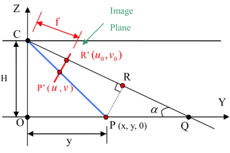
For further analysis, we discuss the spatial relation between the vehicle coordinate and the image coordinate system through two different points of view. Figure 2-3 and Figure 2-4 are the side view and bird’s eye view of the geometric chart between the vehicle coordinate and the image coordinate system.
Fig. 2-3 : Side view of the geometric relation between the vehicle coordinate and the image coordinate system.
Z Y O α y Y Z f P’ (u,v) P (x, y, 0) Q R H O C Image Plane R’( , )u v0 0 X OC α β P (X, Y, 0) (u0,v0) (u,v) Road Plane Image Plane H
Fig. 2-4 : Bird’s eye view of the geometric relation between the vehicle coordinate and the image coordinate system.
Before explaining the formulation of the transformation between the two coordinate systems, some annotation must be introduced about Fig. 2-3 and Fig. 2-4 in advance.
f: Focal length of the camera
u
f 、 f : The scaling factors of the image plane in the horizontal and vertical axis v
H: The distance from the road plane to the camera
α : Tilt angle of the camera β : Pan angle of the camera
( , ): The corresponding point in the image plane is projected from the road surface u v 0 0
( , )u v : The central point of the image plane
In Fig. 2-3, ΔCPR and are similar triangles. With this property, the
spatial relation between two coordinate systems can be derived as follows.
' ' CP R Δ X β R Y β x P (x, y, 0) Q C y R’( , )u v0 0 f P’ (u,v) Image Plane
0 ' ' ( ) sin ( ) sin tan cos ( ) co sin tan v PR PR CR CR h y v v f PQ h h f CQ PQ y α α α α sα α α = − ⋅ − ⋅ ⋅ ⇒ = = − ⋅ − − ⋅ 0 2 0 0
( ) cos sin tan
cos tan ( ) cos sin tan [ ( ) tan ] [tan ( ) ] v v v v v f h y h y h h f h y y f v v f y f v v f h α α α α α α α α α α − ⋅ ⋅ − ⋅ − ⋅ ⇒ = = ⋅ + − − ⋅ ⇒ ⋅ − + ⋅ ⋅ = ⋅ ⋅ − − ⋅ Assume v v f S f
= is the camera constant of the image plane in the vertical axis
0 0 [( ) tan ] ( ) tan v v v v S h y v v S α α − ⋅ − ⋅ ⇒ = − + ⋅ (2-1)
Similar to the above process, the deducing details about Fig. 2-4 will be described in the following.
0
0
' cos
' sin
( ) ( tan ) cos cos sin
cos sin ( tan ) sin cos ( ) tan tan u u PR PR PQ CR CR CQ PQ u u f x y x y y f x y y u u f x y f y x β β x β β β β β β β β β β β ⋅ = = + ⋅ − ⋅ − ⋅ ⋅ ⋅ − ⋅ ⇒ = = ⋅ + ⋅ + − ⋅ ⋅ − ⋅ − ⋅ ⇒ = + ⋅ Assume u u f S f
= is the camera constant of the image plane in the horizontal axis
0 tan tan u u u x y S y x β β − − ⋅ ⇒ = + ⋅ 0 0 [( ) tan ] ( ) tan u u y u u S x S u u β β ⋅ − + ⋅ ⇒ = − − ⋅ (2-2)
Equation (2-1) and (2-2) are the transformation from the point ( u , ) in the image plane to that (x, y, 0) within the road surface in the vehicle coordinate system. However, parts of the parameters in this formulation are unknown. We must make use of some probable approach to estimate those values if the precision of the perspective
phenomenon is adequate.
2.1.2 Applications of Frontal-View Lane Detection
For several years, many researchers worked on driving assistance problem by using the concept of artificial vision. Among those applications about intelligent transportation, automatic navigation has been taken seriously in recent years. For accomplishing this objective with efficient performance, most vision-based methods are to extract the road information by mounting the image sensor on the windshield of the vehicle. Such as the human eye, forward-looking camera can extract the widest field of view than other mounting position around the car body. In general, by detecting the contrast between the white lines and the road, the lane boundary in front of the vehicle can be sufficient to detect. Furthermore, the variation of the lane’s curvature can be predicted in time without resulting in the erroneous following of the vehicle. Besides, some obstacles captured by the camera can be recognized with 2D or 3D techniques of computer vision. Other related works such as keeping the secure distance ahead of the car are based on this system configuration.
2.1.3 Applications of Lateral-View Lane Detection
Some risks of road traffic which occur on highway during the lane-changed maneuver happen easily if another vehicle besides the own one has been overlooked. In other words, drivers have not assured accurately if there is no other vehicle alongside in the blind spot of the lateral view. During the general driving procedure, drivers must keep notifying the frontal field of view so that they forget to check the information of the lateral blind-spot at the same time. In order to overcome this kind
of traffic hazard with efficiency, a camera is mounted at the driver’s outside rear-view mirror to monitor the blind spot and the alongside lane. Approaching vehicles should be detected in time and tracked until they leave the blind spot by this configuration. In addition, this system can restrain the intended lane -changed maneuver and maintain the distance from the lane boundary in the blind spot to the realistic car body without a significant amount of the potential collisions.
2.1.4 Comparison with Two Applications on Vehicle
In addition to the distinct effect of the geometric projection onto the image plane, there are still other different factors and applications between the frontal-view and lateral-view configurations. The four reasons are listed as follows.
(1) The initial purpose has influence on where the camera is mounted:
As explained in section 2.1.2 and 2.1.3, road images extracted from the forward sight of the vehicle can yield more driving information to track the real-time road curvature by the lane-marking modeling. Furthermore, the related data of them has effectively contributed to the system with respect to the assistant navigation. On the other word, the major objective about mounting the camera on the side of the car is to adjust how much is the detecting range of the blind-spot region. This configuration only puts emphasis on judging the approaching car or the lane trajectory near the vehicle, and the variation of the forward road information can be not considered.
(2) The diverse sensation of the driver with respect to two mounting position:
In general, to extract the forward visual information as far as possible, the camera was almost fixed to the windshield. This setting location could easily reduce the eyesight of the driver whether the size of the camera is so small or not. The
disadvantage resulting from the driver’s unfamiliar looking will be concerned with the research about driver analysis. Nevertheless, due to the position of the camera near the rear-view mirror when focusing on extracting the lateral-view content of the vehicle, drivers can be not confused with this experimental environment. In other words, the camera added to the vehicle can not affect the original driving habit of the driver, and the data collected by driver analysis system will still be higher accuracy.
(3) The different extrinsic factors of two locations of the sensing device
Compared with the initial purpose of two configurations, the camera mounted in front of the vehicle must have farther distance from its optical center to the specified lane portion on the road plane than that on the side of the car because of the perspective geometry. In addition, the overtaking cars which crossing the lane are almost captured by the frontal-view image sequences. Therefore, the information of the lane trajectory extracted by the sideward camera can be more complete than the forward one throughout the driving experiment on highway. However, with the headlight switched in the gloomy driving situation, the video collected by the frontal camera can still hold more acceptable luminance information in night vision.
2.2 Definition of Vehicle Blind Spot
Blind spots, in the context of driving an automobile, are the areas of the road that cannot be seen while looking forward or through either the rear-view or side mirrors. Detection of vehicles or other objects in blind spots may also be aided by systems such as video cameras or distance sensors. Throughout the notation in this thesis, the
area of blind spot is only regarded as the rear of the vehicle on both sides. The introduction in this section not only describes the causes of traffic accidents resulted from the blind spot, but discuss how to resonablely establish the region of blind spot by the inherent limitation of the human vision and rear-view mirror.
2.2.1 Traffic Accident Causes of Vehicle Blind Spot
In Taiwan, the types of traffic accidents between two cars on highway are listed in Table 2.1 from [17].
Table 3 : Causes of traffic accidents between two cars on highway.
Year Collision by the
Backward Car Rubbed Collision in the Same Direction Lateral Collision Colliding Collision Others 2001 59.74% 28.57% 2.86% 1.56% 7.27% 2002 62.39% 28.04% 3.04% 1.74% 4.78% 2003 60.82% 27.88% 3.70% 2.34% 5.26%
As shown in foregoing statistics, we can conclude that the lateral and rubbed collisions are both the principal causes of the traffic accidents between the cars. There have been numerous topics focused on how to avoid the forward or backward collision for the vehicle, but the related research for lateral collision is little. When vehicles in the adjacent lanes of the road fall into the range of lateral blind spots, the driver will be unable to see them with only the car’s mirrors. Due to the above reason, drivers must actively rotate their head to extract more information within the region of blind spot. However, the probability of car accident can be raised simultaneously. Therefore, vision-based system can be developed to assist the drivers in keeping away from the lateral danger of vehicles by the image sensor alongside the rear-view mirror.
2.2.2 Limitation of View by Human-Vision
The eyesight of people has obvious difference between the static and dynamic environment due to the variation of the vehicle velocity. In general, the view-angle of the single eyeshot is about 160 degrees when people lie in the stationary scene; the maximum view-angle of the double field of view is enlarged about 180 degrees. Flannagan [18] proposed that the people’s double eyesight should reach to 320 degrees by adding the rotating motion for the head and body of human. According to the statistics from [19], the realistically clear field of view contained two eyes is only about 70 degrees when a normal person situates in the static environment. Nevertheless, the human’s eyesight could frequently vary when people are in the dynamic conditions such as the internal part of the moving vehicle thanks to the tunnel-vision effect. The relationship between the range of human eyesight and the variation of the vehicle velocity is in Table 2.2; the range of field of view between the static or dynamic environment is shown in Fig. 2.5.
Table 4 : The relationship between the field of view and the vehicle velocity.
Speed (km/hr) 40 70 100
70km/hr 65D
100km/hr 40D
40km/hr 100D
210D
Fig. 2-5 : The diagram of the driver’s field of view.
As the information shown in Fig. 2-5, the eyesight becomes greatly narrow when the vehicle is driven at high speed. In other words, the driver can not judge whether there are other vehicles moving on the adjacent road surface or not only by his/her remaining eyeshot on highway as the car velocity raises to 100 km/hr. In this way, drivers induced by the blind-spot hazard will be easily in danger.
2.2.3 Limitation of View by Rear-View Mirrors
In general, the side mirrors of the vehicle are almost used by the planar type. Therefore, the formation of image about the normal rearview mirror is still followed by the principle which describes that the angle of incidence (θi) is the same as that of reflection (θr). In other words, the field of image produced by the rearview mirror is
stretched to 2θ (θ =θi=θr) view-angle projecting into the road surface.
The relationship between the field of view of the side mirror and that of the driver is shown in Fig. 2-6.
70km/hr 65D
40km/hr 100D
100km/hr 40D
Fig. 2-6 : The relation about field of view between the side mirror and the driver. By the geometric relation from Fig. 2-6, when driving at high speed, in order to make the eyesight overlap the reflected field of rearview mirror, the driver must rotate his/her head so as to extract the lateral information as much as possible. However, due to this unnatural motion, the driver’s inattention will not keep his/her eye for the forward state of the vehicle for a long time with the occurrence of traffic accident.
There are two general approaches to extend the range of field of the rearview mirror. The first approach is to increase the distance between the side mirror and the driver. Due to the fixed car-body, this improving effect will be restricted. The second approach is to replace the traditional planar mirror with the curved one. Nevertheless, the distortion effect of the reflected image will be serious due to the curvature of the lens. Through the above discussion, the blind-spot region between the side mirror and the driver can not be easily resolved. For this reason, adding the camera on the side of the car with intelligent vision-based algorithm will still be regarded as the important device of the assistant system for the driver’s safety.
2.3 Principles of Lane Detection
The objective of lane detection method we expected in this thesis is to extract the lane markers without knowing the internal or external parameters of the camera alongside the vehicle in advance. Besides, the sensitivity of the image sensor easily disturbed by the light condition must be suppressed as much as possible. Therefore, developing an adaptive lane-finding system is essential to satisfy the previous demands. First, our system can automatically extract the ROI contained by the road surface only by the image content despite the unknown environmental information of camera. Second, the preprocessing tasks will be able to effectively restrain the noise when driving in the nighttime. Through the property for the view-angle of blind spot, the improving edge operator will be added to acquire the clear lane boundary. Not depending on the distortion of the camera lens which results in the obviously curved lane trajectory even if people drive on the straight road, a piece-wise edge linking model will be developed to mark all information of lanes shown in image sequence.
2.4 Principles of Lane Departure
Warning and Drowsiness Prediction
The part for lane departure warning is to provide some triggers for caution with respect to the driving-off-road behavior through the lateral information of the lane extracted by the lane detection algorithm. After measuring the lateral velocity from the consecutive frames, the warning system will determine when the departure driving occurs based on the lateral displacement and TLC (time to lane crossing.)
experimental results of BRC (brain research center) from NCTU with the realistic driving video. In order to estimate the lateral location of lane where the driver gets used to navigate on the straight road, we construct the single Gaussian model to simulate the stable-state range about the lane position. Then, the additional updating mechanism will contribute to the systematic adaptation even if the driver changes his/her driving habits. At last, the proportional gauge of the drowsy degree we proposed will show if the driver has higher or lower probability in the drowsy state at that moment with the amount of reflection time measured by the lane position over the stable-state region.
3
Chapter 3
Lane Detection
3.1 Overview
Figure 3-1 shows the flow chart of lane detection. At the beginning of this architecture, because we merely aim at the monochromatic information of each frame to process, the RGB coordinate will be transformed into the YCbCr one so that the illumination component will be totally retained. Then, the automatic mechanism about searching the ROI (region of interest) of the image content will be described in Section 3.2.1. The preprocessing step about de-noising will be presented in Section 3.2.2.
Next to the processing step, the flow will enter the principal detection parts. Due to the mounting position of camera on the side of the car, the image captured by that device will contain most of the lateral-view information next to the wheels. In other words, only one lane trajectory which is the most closed to the vehicle can be apparently seen. An edge detection operator will be developed to adapt to the geometry relationship of the camera based on the property of view-angle in Section 3.3. In addition, the binarization step we proposed in this section will depend on the spatial relation with respect to the perspective effect. To eliminate the blind-spot region as much as possible, we choose the fish-eye camera for enlarging the field of view with some obvious distortion result. Therefore, the adaptive edge-linking model demonstrated in Section 3.4 will overcome the serious problem whether the lane boundary in the image sequences is straight or not.
3.2 Preprocessing
3.2.1 Automatic ROI Extraction
Before discussing how to search for the lane-marking, the step of color transformation must be executed. In general, most of the algorithms shown in the past theses with respect to lane detection are only considered the grey-level component. This reason is that the contrast between the lane boundary and the normal road plane can be easily seen by normal people as usual even if the colors of lanes are not necessarily the same. As a result, the information of luminance for each frame must be stored in our system by the RGB-to-YCbCr transformation. On the other hand, the remaining chrominance components such as Cb and Cr are not taken seriously due to the insensitive perception about human eyes. The formulation of transformation can be described by
(3.1) As shown in Section 2.1.1, equation (2-1) and (2-2) tell us the relationship of geometric transformation which demands the known information of camera, such as the height, pan-tilt angle, and the internal focal-length of the camera, between the image coordinate and the vehicle coordinate systems. Some methods proposed in the previous works have to compute the curvature of the realistic road plane or to estimate the lane shape effectively by these intrinsic or extrinsic parameters. However, an adaptive system can not be sensitive to the variation of the camera mounting position for the aspect of application and commerce. For instance, the systematic performance
0.257 0.504 0.098 16 0.148 0.291 0.439 128 0.439 0.368 0.071 128 Y R Cb G Cr B ⎡ ⎤ ⎡ ⎤ ⎡ ⎤ ⎡ ⎤ ⎢ ⎥ ⎢= − − ⎥ ⎢ ⎥ ⎢⋅ + ⎥ ⎢ ⎥ ⎢ ⎥ ⎢ ⎥ ⎢ ⎥ ⎢ ⎥ ⎢ − − ⎥ ⎢ ⎥ ⎢ ⎥ ⎣ ⎦ ⎣ ⎦ ⎣ ⎦ ⎣ ⎦
should be not influenced by the distance between from the rear-view mirror and the road surface about various vehicles.
To take this target, we hope that our detection algorithm can automatically determine the ROI (region of interest) contained the whole lane trajectory on the road surface only by the image content with lateral view-angle. The chosen range of ROI should be unchanged by the later information of image sequences whether some new moving objects are captured or not. Figure 3-2(a) demonstrates the realistic frame acquired by the camera alongside the side mirror. Through being concerned about the image content, the fixed parts within it might be regarded as the evidence for ROI extraction. In our opinion, the sideward car body with constant area throughout the image sequences and the horizon relative to the road plane both correspond to the fixed condition. Therefore, the approximately location of ROI will be determined by the edge information of them.
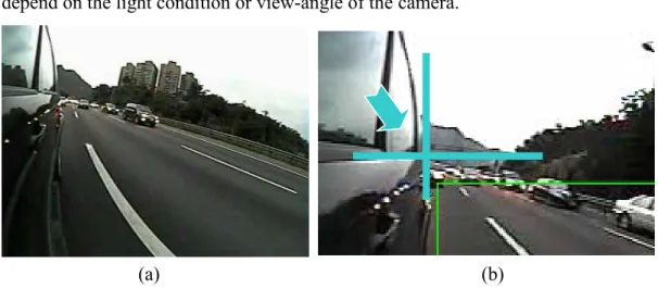
The definition of ROI is that a rectangle region which extends its width to the location next to wheels contains all the lane shapes in the image. In general, the height of ROI is below the vanishing point situated in the horizon closed to the border of vehicle’s window. This 2D geometry with respect to the above characteristics can not depend on the light condition or view-angle of the camera.
(a) (b)
Fig. 3-2 : (a) The image acquired by the camera alongside the rearview mirror. (b) The upper left point of ROI next to the boundary of the vehicle window.
Figure 3-2(b) shows the location of the upper left point of ROI between the boundary of the window and the vanishing point. In this figure, the portion of green rectangle is shown as ROI, and the intersection of the marking cross stands for the key point to determine where the range of ROI has covered. In this case, the 2-D gradient operator will be used to extract the position of key point by considering the boundary information of the vehicle window. Hence, we use only two of eight-directional Sobel masks for detection due to the obvious edge of the window in the horizontal and vertical aspects, as follows:
x, y : coordinate values of each pixel in the x and y axis f (x ,y) : the intensity of this pixel
[
( 1, 1) 2 ( , 1) ( 1, 1)] [
( 1, 1) 2 ( , 1) ( 1, 1)]
x G = f x− + + ⋅y f x y+ +f x+ + −y f x− − + ⋅y f x y− +f x+ − (3.2) y[
( 1, 1) 2 ( 1, ) ( 1, 1)] [
( 1, 1) 2 ( 1, ) ( 1, 1)]
y G = f x− − + ⋅y f x− y +f x− + −y f x+ − + ⋅y f x+ y +f x+ + (3.3) y (a) (b) Fig. 3-3 : The mask type of (a)G . (b)x Gy.The two mask types are shown in Fig. 3-3. Figure 3-4 displays the results of Sobel edge detection with Gx and Gy. After extracting the border of the window from Fig. 3-4 (b) to Fig. 3-4(d) with thresholding, the coordinate values of the key point in the x- and y- axis will be founded to determine the range of ROI by computing which row and column retain the most edge pixels along the horizontal and vertical direction individually. This process can be expressed as:
( )
0 0 255 if ( ( , )) or ( ( , )) , 0 else where ( , ) x y key h w y x G I x y TH G I x y TH I x y I x y TH w h = = > > ⎧ = ⎨ ⎩ = ⋅∑∑
(3.4) (3.5)The ratio of to the image width is closed to 0.5, and that is the same case as the ratio of h to the image height. Due to the more edge pixels naturally existed along the horizon in the horizontal axis and the perpendicular border of vehicle in the vertical axis, an intersection point of the car window can be found out by searching in the x-y direction respectively. The detecting results with different light conditions and view-angles are shown in Fig. 3-5.
w
(a) (b)
(c) (d)
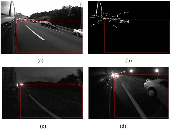
Fig. 3-4 : (a) Original image. (b) Edge detection by Gy. (c) Edge detection by Gx. (d) Edge detection by Gx+Gy.
(a) (b)
(c) (d)
Fig. 3-5 : (a) Day light. (b) ROI extraction of (a). (c) ROI extraction at night. (d) ROI extraction with different view-angle in the nighttime.
Although the horizontal border of vehicle window may be unclear in the worst conditions which the illumination from the car and street light has not adequate at night, the extracting result is still steady since the edge information of horizon can be replaced to obtain the similar position in the x-axis, as shown in Fig. 3-5(c) and (d).
3.2.2 De-noise Processing in Spatial and Temporal
Domain
The quality of image sequences collected by the vision-based sensing device will be almost subjected to this challenge of the variance of light conditions, such as day or night situation. Because the problems about high-frequency noise will be serious for some driving environment due to the photosensitivity of cameras, especially on
night vision. Therefore, the preprocessing step for eliminating the noise effect must be considered in the detecting architecture if the system is expected to work robustly all day long.
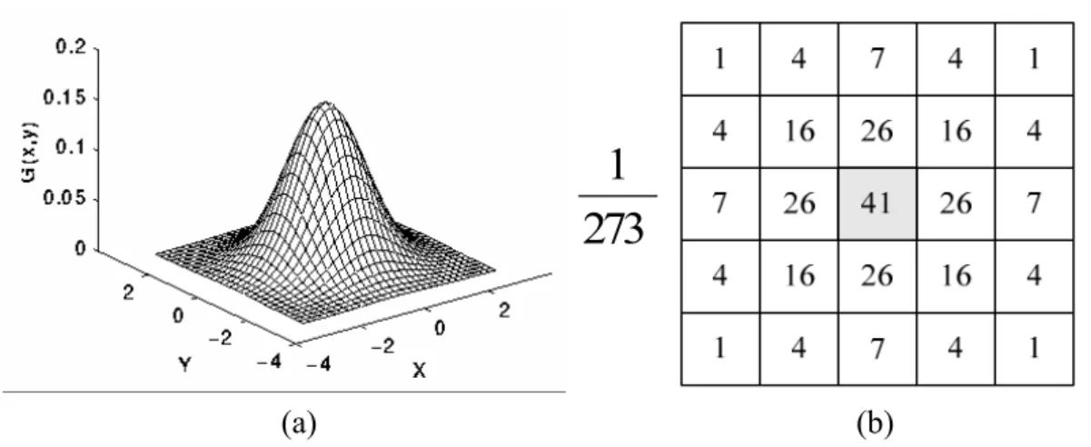
In general, a low-pass filter can be implemented before the process which is used to extract the information about the boundary, texture, or shape of the interesting objects within the frame. Since the frame is stored as a collection of discrete pixels, we need to produce a discrete approximation to the chosen filter-type before the convolution step. Hence, the Gaussian smoothing operator which is a 2-D point-spread function achieved by convolution is used for this de-noising task in our system. The isotropic form of Gaussian is shown as below:
2 2 2 2
1
( , )
exp(
)
2
2
x
y
G x y
πσ
σ
+
=
−
(3.6) is the standard deviation of this functionwhere σ
The diagram of this distribution is shown in Fig. 3-6(a). Moreover, this function has been assumed with a zero mean. In principle, the Gaussian distribution is non-zero everywhere, but its value is closed to zero more than about three standard deviations from the mean centered at the distribution. Therefore, we can truncate it as the mask-type at the specific pixel of each frame. Figure 3-6(b) shows a suitable integer valued convolution mask of Gaussian where σ =1. The Gaussian filter outputs a weighted average of the neighborhood of each pixel. It can provide gentler smoothing and preserves edges better than the normal-sized mean filter due to the distinct size between 5x5 and 3x3. On the other hand, by choosing an appropriately size of Gaussian filter determined by the standard deviation, more range of spatial frequencies is still preserved in the image after filtering because its Fourier form is itself a Gaussian. However, over-wide region contained in the filter will result in the
serious blur effect of the image content. Therefore, the 5x5 principal type of Gaussian mask is still adopted in this part.
273
1
(a) (b)
Fig. 3-6 : (a) 2-D Gaussian Distribution with mean(0,0) and σ=1. (b) Suitable 5x5 mask of Gaussian filter with σ =1.
Some results of edge detection which describes the details in the next section is preprocessed by Gaussian and Mean filter as shown in Fig. 3-7. Compared with (c) and (d), the extracting method of the lane boundary will be easily disturbed by the remaining noise if the smoothing filter can not effectively remove the high-frequency perturbation.
(a) (b)
(c) (d)
Fig. 3-7 : (a) Mean filter. (b) Gaussian filter. (c) Edge detection after (a). (d) Edge detection after (b).
for the preprocessing tasks, especially the night environment. To achieve the objective that the effect of the proposed lane detection method in this thesis must be independent on the variation of external light conditions, the time-averaging process focused on the current and previous frames will be added behind the Gaussian smoothing work. The integrated de-noising procedure is demonstrated in Fig. 3-8.
Fig. 3-8 : Flow chart of the complete preprocessing steps.
The preprocessing work
3.3 Lane Boundary Detection
3.3.1 Edge Detection
The objective in this section is to find the features of lane marker from the information of image. Through the observation, lanes must have some apparent properties about its boundary. The most obvious reason of them is that the lane markers must be brighter than the neighborhood road surface even if they are with various color information. Then, the lane shapes in the image are almost presented as slender types. In other words, extracting the lane boundary is an important step to locate the realistic lane position throughout the video by the foregoing two factors.
The determination of edge detection operators need to be considered the suitable and effective performance for the image contents. Y. Wang [7] and [10] select Canny operator to locate the position of pixels where the significant edge information of
lanes exists by considering the gradient characteristics at the same time. However, using this operator will accompany the obvious computing load since the judging mechanism about the orientation and magnitude of each candidate edge in the whole frame. On the other hand, Kreucher [20] provides a frequency-based extracting method to find the diagonal dominant edges through the partly DCT coefficients. This special concept is so intuitive that the components of edges determined by DCT may be not related to the local information more closely than the common gradient operators, especially about the contents of video acquired by the camera on the side of the vehicle without fixed edge direction of lane markers. By giving the consideration to effects about the systematic performance and the adaptation of video with various view-angles, the LoG (Laplacian of Gaussian) operator is implemented in this step.
LoG is an associative convolution operation which convolves the Gaussian smoothing filter with Laplacian filter of all, and then convolve this hybrid type with the image to achieve the required result for edge detection. As an approximated second-order derivative, the Laplacian mask can highlight the regions where the intensity of pixels contained by the boundary of objects changes rapidly. Nevertheless, this operator can not be used for edge extraction thanks to the higher sensitivity of noise. To reduce this effect, the image has often smoothed by Gaussian before applying the Laplacian mask. Because the second derivative is a linear operation, the hybrid mask of two filters is similar to convolve the Gaussian function first and compute the Laplacian of the result. The 2-D LoG function is shown as follows:
2 2 2 2 2 2 2 2 2 2 2 2 2 4 2 ( , ) ex p ( ) 2 ( , ) ( , ) ( ) ex p ( ) 2 x y f x y f f L o G x y f x y x y x y x σ σ σ σ ⎡ ⎤ ⎢ ⎥ ⎢ ⎥ ⎣ ⎦ + = − − ∂ ∂ = ∇ = + ∂ ∂ + − + = − ⋅ − y (3.7)
1 2 1 2 -2 0 2 4 6 8 1 0 1 2 1 4 1 6 0 0 -1 0 0 0 -1 -2 -1 0 -1 -2 16 -2 -1 0 -1 -2 -1 0 0 0 -1 0 0 Z X Y (a) (b)
Fig. 3-9 : (a) 5x5 mask approximation of LoG. (b) 3-D plot of (a).
The 5x5 mask approximation to the LoG function and its 3-D plot is shown in Fig. 3-9. By further observing the property of blind-spot view image from the camera alongside the rear-view mirror, the included angle from the edge of lane to the vertical Y-axis of the image plane must be within the range of degree from . Compared with other gradient operators, LoG mask has no orientation so that it can not adapt to some specific edge directions of the object. So the additional 5x5 mask similar to the form of the sobel-mask with tilt angle of 45 degree is provided to be combined with the previous LoG mask to adapt to the lateral-view image environment. The convolving relation is explained in the following:
0 to 90D D ( , ) ( , ) ( , ) ( , ) ( , ) ( , ) ( , ) ( , ) I x y ∗ f x y +I x y ∗g x y ⇔I u v F u v +I u v G u v ( , ) ( , ) ( , ) [ ] ( , )[ ( , ) ( , )] I x y ∗ f x y + g x y ⇔ I u v F u v +G u v (3.8)
where ( , ) : the LoG mask, g( , ) : the additional 5x5 combining mask
f x y
x y
The 3D-plot of new combined mask f x y( , )+g x y( , ) will be shown in Fig.
3-10(b). Compared with Fig. 3-9(b), this distribution not only maintains most part of the LoG shape, but also be added the identity of orientation for the blind-spot view due to the “slant” shape in Fig.3-10(b). The results of edge extraction for lane
boundary between the LoG and the new combined mask are demonstrated in Fig. 3-11. According to the result from Fig. 3-11(d), only the intra-boundary of the lane can be extracted, and this property will contribute to link the lane trajectory described in the later section. 1 -4 -2 0 2 4 6 8 1 0 1 2 1 4 1 6 2 1 2 0 -1 -2 -3 -4 1 0 -1 -2 -3 2 1 0 -1 -2 3 2 1 0 -1 4 3 2 1 0 Z X Y (a) (b)
Fig. 3-10 : (a) The additional mask for LoG combination. (b) 3-D plot of the new 5x5 combined mask.
(a) (b)
(c) (d)
Fig. 3-11 : (a) The original image. (b) Gaussian smoothing within the ROI of (a). (c) Result of LoG mask. (d) Result of the new combined mask.
extraction. There are two conditions determining which the pixel can be retained in the image:
if I(k)=255 AND I(k+1)=255
I(k+N)=0 where N is a little larger than 2 else if I(k)=255 AND k>P(i)
I(k)=0 where P(i) is the point corresponed to ⇒
⇒ the lane boundary of the row
else
⇒ I(k)=255
The edge-finding approach to determine the location of P(i) will be introduced in Section 3.4.
3.3.2 Adaptive Threshold Determination by Distinct
Spatial Region
The pixels within the ROI can be extracted for the image processing tasks in our system. According to the perspective geometry, the length or width of the lane markers within ROI is not the same with each different position. In other words, the lane boundary in the bottom part of ROI is always wider and longer than that in the up part. By considering the transformation effect, the adaptive mechanism is developed to adjust the threshold for different sub-regions, and the size of them depends on ROI.
After processed by edge extraction, the image needs to be decided the threshold for more obvious detecting result. Due to the evidently contrast between the lane markers and the neighborhood road surface, the gradient magnitude of lane boundary caused by the edge operator is usually larger than other locations. Therefore, in this section the values of mean and standard deviation computed by each row within the ROI will be selected as the threshold for different region.
for one standard deviation from the mean will account for about 68% of the whole set. Besides, the range will account for about 95% if it contains the distance for two standard deviations from the mean. For each row within ROI in the image, the threshold value is still selected by referencing above scattered property since the gradient magnitude of lane markers is certainly higher than that of the normal road surface. That is,
i (0, width of ROI) i (0, width of ROI)
( ) Mean ( , ) Standard deviation ( , ) where k=2,
j : j-th row of ROI,
( , ) : the value of each pixel within ROI after the edge
Threshold j f i j k f i j f i j ∈ ∈ = + ⋅ detection. (3.9)
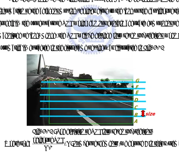
The performance of the binarizing approach may be dependent on the edge information of the adjacent moving vehicles close to the lane or the car-light of them, especially the upper part of ROI which can not contain adequate component of the magnitude of lane. Hence, the ROI will be divided into seven sub-regions when it is automatically extracted in the first frame of video, as illustrated in Fig. 3-12
A B C D E F G size
Fig. 3-12 : The division of ROI into seven sub-regions.
height of ROI
Where size= , N: number of segments (we choose 7 in this system) N-1
In this way, the values of thresholds situated in different location are selected by tuning the mean value of each-row pixels and the arrangement of magnitude for them
are from the bottom to the top sub-region, as described in the following:
(
i (0, width of ROI))
i (0, width of ROI)( ) Mean ( , ) Standard deviation ( , )
Threshold j f i j
α
k f i j ∈ ∈ = − + ⋅ (3.10) i (0, width of ROI) 0 =0.1 n (Standard deviation ( , )) , k f i j k α ∈ = ⋅∑
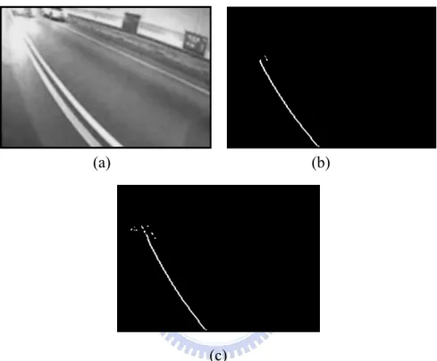
⋅ where : n-th sub-region of R .n OI (a) (b) (c)Fig. 3-13 : (a) The image is photographed in a tunnel. (b) Lane-marker extraction without considering the sub-region threshold. (c) Lane-marker extraction with considering the sub-region threshold.
Figure 3-13(a) shows an imaging environment about driving in a tunnel. The original lane boundary in the upper region is not easily seen due to the disturbance of the car-light from the backward vehicle, as shown in Fig. 3-13(b). This overexposure effect will be improved by considering the tuning parameter (α ) in Fig. 3-13(c).
3.4 Lane-Finding Algorithm
Since the edge information of lane markers has been acquired by the foregoing demonstration, marking and tracking the lane trajectory within ROI can be succeed by such pixels lying on the sides of lane boundary in the image. There have been some researches for lane-model construction. Y. U. Yim and S. Y. Oh [21] use the starting position, direction, and saturation of the lanes regarded as the three features to initialize the lane vector and find the most probable lane trajectory by Hough Transform. Roland Chapuis [25] uses the statistical model to specify the detection ROI in order to narrow the searching area of lane markings. Different from the method merely about the image processing, the lane geometry is taken into the fitting of the lane model provided by A. Lopez [28]. D. J. Kang [30] combines the vanishing point of the road from the frontal camera with Hough Transform for lane tracking.
Based on the objectives for real-time tracking and low-cost computation, a piece-wise edge linking model we proposed in this chapter is effective for lane-shape marking whether the lens-distortion of camera is serious or not.
3.4.1 Distortion Effect of Fish-Eye Camera
A fish-eye lens with a wide angle that takes the extremely wide field of view can cause the hemispherical effect of the image. All the ultra-wide angle lenses of the fish-eye cameras suffer from some amount of distortion. In order to contain the blind-spot region on the side of the car as much as possible, we choose a fish-eye camera as a sensing device for image acquisition.
The distortion effect of lane boundary resulted from the fish-eye camera is shown in Fig. 3-14, which displays the different curvature of lane-shape whether the distance between the lane and the vehicle is so closed or not. Tsai [33] and Hartley [34] provide the algorithms for fish-eye calibration by the internal or external parameters of the camera. However, this kind of information can not be known in advance in our systematic architecture. In other words, the lane-trajectory finding algorithm in this thesis needs to overcome the inherent problem without considering additional computing load for calibration.
Fig. 3-14 : The different curvature of lane in (a) the lane boundary is close to the car-body. (b) The lane boundary is far to the car-body.
3.4.2 Hough Transform
The classical type of Hough transform is to identify the edge or boundary of lines in the image. This principle is to transform the X-Y coordinate system into the r-θ parameter space, where r represents the small distance between the line and the origin of the image, and θ is the angle of the locus vector from the origin to this closest point. The relationship of the transformation about two coordinate systems is shown in Fig. 3-15. According to equation (3.11) from this figure, they can determine if the point A and B are colinear with the same r and θ. Besides, equation (3-12) is to determine if the line segment formed by A and B is collinear with that formed by C
and D by judging the condition that the parameter d is smaller than a threshold.
1
cos
1sin
2cos
2sin
r
= ⋅
x
θ
+ ⋅
y
θ
= ⋅
x
θ
+
y
⋅
θ
(3-11)( cos
sin )
d
= − ⋅
r
x
θ
+ ⋅
y
θ
(3-12) (x3, 3) C y (x1, 1) A y (x2, 2) B y (x4, 4) D y Θ ΘFig. 3-15 : The diagram of relationship between the x-y and r-θ coordinate systems.
3.4.3 Piece-Wise Edge Linking Model
Qing Li [22] and C. H. Yeh [24] still apply the Hough transform to track the lane markers which can not be deformed in the image captured by the normal camera. However, due to the distinct curvature with the fish-eye lens, it is impossible to take Hough transform into our system. Hence, the novel approach for lane modeling needs to be considered the geometric effect of ROI and the connectivity of the lane markers with robustness and adaptation.
(a) (b)
Fig. 3-16 : (a) Seven sub-regions automatically segmented within ROI. (b) The flow chart of the piece-wise edge linking model.
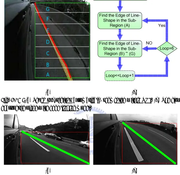
(a) (b) B C D E F G A
Fig. 3-17 : (a) Seven sub-regions segmented within ROI. (b) The flow chart of the piece-wise edge linking model.
Figure 3-17 shows the two different size of ROI is caused by the variation of the intrinsic and extrinsic setting of camera. In general, the width of ROI depends on the yaw angle of camera, and the height of that depends on the pitch angle or the distance from the mounting position near the rearview mirror to the road plane. Although those parameters can not be taken in our system, we still find the property that the lane boundary in the image must extend to the upper-left part of ROI even if the lateral position estimated from the lane marker is not the same through the image sequences.
TH
KeyAngle−RegAngle>θ
Fig. 3-18 : The flow chart for finding the line-shape in the bottom sub-region (A).
2 TH
KeyAngle RegAngle− >θ