Symbiotic Structure Learning Algorithm for
Feedforward Neural-Network-Aided Grey
Model and Prediction Applications
SHIH-HUNG YANG1, WUN-JHU HUANG1, JIAN-FENG TSAI2, AND YON-PING CHEN3
1Department of Mechanical and Computer Aided Engineering, Feng Chia University, Taichung 40724, Taiwan 2Department of Electrical Engineering, National Formosa University, Huwei 63201, Taiwan
3Department of Electrical Engineering, National Chiao Tung University, Hsinchu 30010, Taiwan Corresponding author: Shih-Hung Yang ([email protected])
This work was supported by the Ministry of Science and Technology of the Republic of China, Taiwan, under
Contract MOST 105-2221-E-035-014-, Contract MOST 105-2218-E-150-003-, and Contract NSC 102-2511-S-009-011-MY3.
ABSTRACT The learning ability of neural networks (NNs) enables them to solve time series prediction problems. Off-line training can be applied to design the structure and weights of NNs when sufficient training data are available. However, this may be inadequate for applications that operate in real time, possess limited memory size, or require online adaptation. Furthermore, the structural design of NNs (i.e., the number of hidden neurons and connected topology) is crucial. This paper presents a novel algorithm, called the symbiotic structure learning algorithm (SSLA), to enhance a feedforward neural-network-aided grey model (FNAGM) for real-time prediction problems. Through symbiotic evolution, the SSLA evolves neurons that cooperate well with each other, and constructs NNs from the neurons with hyperbolic tangent and linear activation functions. During construction, the hidden neurons with the linear activation function can be simplified to a few direct connections from the inputs to the output neuron, leading to a compact network topology. The NNs share the fitness value with participating neurons, which are further evolved through neuron crossover and mutation. The proposed SSLA was evaluated through three real-time prediction problems. Experimental results showed that the SSLA-derived FNAGM possesses a partially connected NN with few hidden neurons and a compact topology. The evolved FNAGM outperforms other methods in prediction accuracy and continuously adapts the NN to the dynamic changes of the time series for real-time applications.
INDEX TERMS Symbiotic evolution, structure learning, neural network, grey model, prediction.
I. INTRODUCTION
Time series prediction is a challenging problem when predict-ing future values accordpredict-ing to past observations. Neural net-works (NNs) have been developed to cope with the time series forecasting problems because of their learning ability [1]. NNs are constructed from numerous interconnected process-ing units (called ‘‘neurons’’) that imitate biological neural systems. These networks are also data-driven, in that they derive previously unknown input–output relationships from training examples [2], [3], and they can therefore approx-imate functions without prior knowledge if sufficient data are available. This characteristic makes them practical for solving various prediction problems, because acquiring time series data is typically easier than producing reliable theo-retical estimations about underlying functions. However, the
structural design of NNs (i.e., the number of hidden neurons and connected topology) is crucial [4]. A NN with a complex architecture may easily fit a training data set but yield a poor generalization for an actual testing data set because of overfitting. However, although a NN with a simple archi-tecture may save computational costs and processing time, it may have insufficient storage capability to precisely predict time series [5]. Therefore, the ideal structure of NNs remains debatable.
A NN consists of a set of interconnected neurons with a fully or partially connected architecture. Researchers have recently endeavored to investigate partially connected NNs for prediction problems [6]–[8], and have shown that fully connected NNs may possess unnecessary connections that lead to a complex structure and longer training times.
Therefore, studies have suggested reducing the number of redundant connections and neurons to reduce the complexity of the NN and improve their generalization ability [9]–[11]. With a growing interest in bioinspired techniques, numerous approaches have been developed for designing the structure of NNs along with the connection weights [12], [13]. These techniques first evolve both the structures and weights of NNs offline, and then apply the trained NNs to prediction problems.
The offline training of NNs has been successfully applied to many prediction problems when sufficient training data are available [14]. However, this may be inadequate for applica-tions that operate in real time, possess limited memory size, or require online adaptation [15], [16]. For example, a very short-term load forecasting network in smart grid applications targets a time horizon of a few minutes to an hour [17]. To overcome this problem, in a previous study, we developed a feedforward neural-network-aided grey model (FNAGM) for real-time prediction [18]. The FNAGM performs one-step-ahead prediction by a first-order single variable grey model (GM(1,1)) [19], and compensates for the prediction error by the NN according to the complementary advan-tages of the GM(1,1) and the NN. Furthermore, the FNAGM adopts online batch training to continuously adapt the NN to dynamic change.
Notably, the FNAGM employs a fully connected NN wherein the number of hidden neurons is determined through a trial-and-error process. The prediction ability of the FNAGM greatly depends on its architecture. When the com-plexity of the FNAGM increases, the online batch training (a key technique of the FNAGM) requires longer computation time and thus may be impractical for real-time applications. Conversely, a FNAGM with too-small architecture might make inaccurate predictions because of its limited ability to process information. Therefore, a flexible and automatic design is necessary for FNAGMs to achieve short computa-tion times in online batch training and improve the general-ization ability for real-time prediction applications.
Symbiotic evolution has been applied to design the structure of partially connected NNs [9], which is an implicit fitness-sharing algorithm adopted in immune system mod-els [20]. In addition to NNs, many studies have applied symbiotic evolution to develop efficient solutions for fuzzy controllers and neurofuzzy systems [21]–[25]. These stud-ies have demonstrated the efficiency and feasibility of sym-biotic evolution in structure learning. In general evolution algorithms, each individual denotes a complete solution to a problem. By contrast, each individual in symbiotic evolution denotes a partial solution to a problem; complete solutions are constructed from several individuals. The partial solu-tions can be regarded as specializasolu-tions that ensure diversity and prevent suboptimal convergence. As indicated earlier, the fitness and performance of a neuron (partial solution) is determined by how well it cooperates with other neurons in the same NN (complete solution). Notably, a neuron that cooperates well with one set of neurons may cooperate poorly
with other sets of neurons. One previous study [9] proposed using symbiotic adaptive neuron evolution to construct NNs by adopting a population of neurons that were each regarded as a partial solution for the NNs. Because the number of hidden neurons should be assigned prior to the evolution process, this algorithm is applicable to a NN when the number of hidden neurons is known. To the best of our knowledge, constructing a FNAGM, including a partially connected NN with considerably fewer hidden neurons and connections in order to reduce computation time for real-time applications, remains an open research problem.
This paper presents a novel algorithm, called the symbiotic structure learning algorithm (SSLA), for designing partially connected NNs that can be used in a FNAGM for online learning and real-time prediction applications. This algorithm evolves neuron and network populations to construct the topology of the NN through symbiotic evolution. The acti-vation functions used in the hidden neurons can be hyper-bolic tangent functions and linear functions. The neurons are evolved through neuron crossover and mutation, during which their fitness is assigned according to their fitness shar-ing within the NN. The proposed SSLA does not develop NNs with a fixed number of hidden neurons, but rather constructs NNs of various sizes by selecting neurons from the neuron population. We argue that evolved, partially connected NNs have more efficient information-processing capabilities per connection than fully connected NNs in online prediction problems. Moreover, the evolved NN described herein helps the FNAGM further reduce the computation time of the online batch training.
The remainder of this paper is organized as follows. Section II gives an overview of the FNAGM. Section III describes the SSLA for designing the FNAGM for predic-tion purposes. Secpredic-tion IV presents the experimental results obtained by the SSLA for three prediction problems. Finally, Section V presents some concluding remarks.
II. FEEDFORWARD NEURAL-NETWORK-AIDED GREY MODEL
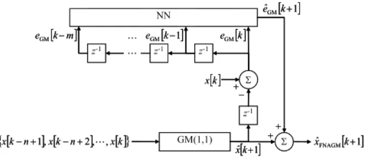
This section briefly describes the FNAGM [18], which adopts a NN to reduce the prediction error of the GM(1,1) through online batch training.1First, a discrete data sequence {x [k − n + 1] , x [k − n + 2], · · · , x [k]} of length n ≥ 4 is acquired. The GM(1,1) estimates the one-step-ahead predic-tive value as ˆx [k + 1]. The prediction error of the GM(1,1) can be computed as eGM[k + 1] = x [k + 1]− ˆx [k + 1] in the
subsequent time step. Once m prediction errors are obtained, the NN estimates the prediction error of the GM(1,1) eGM[k + 1] online, estimated as ˆeGM[k + 1], by using the
mprevious prediction errors for k ≥ n + m. Finally, a one-step-ahead predictive value of the FNAGM, ˆxFNAGM[k + 1],
is obtained by summing ˆx [k + 1] and ˆeGM[k + 1], which
should be more accurate than ˆx [k + 1]. The configuration of
1Describing the GM(1,1) in detail is beyond the scope of this paper; details
FIGURE 1. Configuration of the FNAGM.
the FNAGM prediction is shown in Fig. 1, where z−1denotes a time delay.
The FNAGM adopts online batch training to update the weights of the NN. This training acquires a fixed number of previous prediction errors online and updates the weights in batch mode at each time step. Thus, the FNAGM can improve the prediction error of the GM(1,1) from the limited number of batch training patterns acquired online within a limited computation time. The batch training pattern at time step k consists of r training patterns and is expressed as
Bk = {Pk−r+1, Pk−r+2, . . . , Pk} for k> n + m (1) where Pj = {u [j], eGM[j]} is the jth training pattern,
including input vector u[j] = [eGM[j − m]eGM[j − m +
1]. . . eGM[j − 1]]T and target eGM[j]. Additionally, r =
min {k −(n + m) , N} where N > 1. Notably, the size of the batch training pattern Bkvaries with the number of available training patterns for n + m + N > k > n + m, and is fixed at N for k ≥ n + m + N .
The Levenberg–Marquardt algorithm [27] is then adopted to update the weight vector of the NN, v[k], for k > n + m as follows:
v [k + 1] = v[k] −hGT[k] G[k] +µ[k]I i−1
GT [k]ε [k] (2) whereε[k] is an error vector of the NN, G[k] is the Jaco-bian matrix, andµ[k] is a positive scalar parameter. The jth component ofε[k] is computed as εj[k] = eGM[j] − f (v[k],
u[j]), j = k − r + 1, k − r + 2, . . . , k, with respect to Pj, where f represents an input–output relationship of the NN. The Jacobian matrix is determined as
G [k] = ∂ε [k] ∂v [k] = ∂εk−r+1[k] ∂v1[k] ∂εk−r+1[k] ∂v2[k] · · · ∂εk−r+1[k] ∂vq[k] ∂εk−r+2[k] ∂v1[k] ∂εk−r+2[k] ∂v2[k] · · · ∂εk−r+2[k] ∂vq[k] ... ... ... ... ∂εk[k] ∂v1[k] ∂εk[k] ∂v2[k] · · · ∂εk[k] ∂vq[k] (3)
The online batch training analyzes the previous and current errors,εj[k−1] andεj[k], respectively, which are computed using the same training pattern Pj; subsequently, µ[k] is adjusted as follows: µ [k + 1] = µ[k]/β, if Xk−1 j=k−sε 2 j[k]< Xk−1 j=k−sε 2 j[k − 1] µ[k] · β, if Xk−1 j=k−sε 2 j[k] ≥ Xk−1 j=k−sε 2 j[k − 1] (4) whereβ > 1, s = min {N − 1,k − n − m − 1}, and k ≥ n + m +2. As the current error improves,µ[k] becomes lower; otherwise,µ[k] increases. Consequently, the FNAGM can not only predict signals but also continuously learn to improve the prediction error through online batch training. A stepwise procedure of the FNAGM is described in [18].
FIGURE 2. Architecture of the proposed forecasting system.
III. SYMBIOTIC STRUCTURE LEARNING ALGORITHM
This section presents the novel forecasting system com-posed of structure learning and online parameter learning, as shown in Fig. 2. The proposed system first evolves the structure of the NN of the FNAGM by applying the SSLA, and then performs online batch training on the evolved NN. The SSLA determines the number of hidden neurons and the connected topology of the NN based on a small time series data set acquired for offline structure learning. Once the structure learning is completed, time series data are continu-ously acquired for online prediction and parameter learning. In other words, the evolved FNAGM not only predicts the time series but continuously adapts itself to dynamic changes in the time series by performing online batch training. The SSLA consists of three phases, namely initialization, evalua-tion, and reproducevalua-tion, which are described in the following sections.
A. INITIALIZATION PHASE 1) CODING
The initial step in the SSLA is the coding of a neuron and a NN. Two populations are used in the SSLA: the neuron population and the network population. In the neuron popula-tion, each individual represents a neuron that denotes a partial solution to a NN. Each individual consists of numerous genes that represent the weights and activation function. Consider an example prediction problem with four inputs. As shown in Fig. 3, each individual consists of seven genes: wo, a, whb, wh1, wh2, wh3, and wh4, which represent the output weight,
activation function type, weight connected to the bias, and weights connected to four inputs, respectively. The activation function type indicates which activation function the neuron uses (1 = hyperbolic tangent function; 0 = linear function). Notably, some neuron weights in Fig. 3 are zero, which means that the weights are not connected to the neurons and the neurons are only partially connected. Fig. 4 depicts the three example neurons of Fig. 3.
FIGURE 3. Coding of a neuron in the neuron population and three examples.
FIGURE 4. Graphical representation of three example neurons in the neuron population.
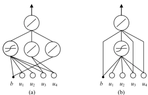
In the network population, each individual represents a NN, which is constructed from the neurons in the neuron population. An example NN with three hidden neurons is shown in Fig. 5a. The output of the NN is obtained by sum-ming the outputs of the three hidden neurons. As illustrated, the NN has a partially connected topology and consists of various activation functions. Because the output of the neuron with the linear activation function is the linear combination of the inputs, the NN in Fig. 5a can be simplified as the equivalent NN shown in Fig. 5b, where the hidden neurons with the linear activation function are transformed into only a few weights directly connected to the output neuron. For example, Neuron C in Fig. 4 can be simplified as the output bias and Neuron B allows u3and u4to directly connect to the
output neuron. Therefore, the SSLA can result in an arbitrary feedforward NN.
FIGURE 5. (a) NN constructed with three neurons. (b) Equivalent NN model.
2) CREATING NEURON AND NETWORK POPULATIONS The SSLA first creates a neuron population by randomly generating Npneurons with the weights and activation func-tion type randomly assigned. Some of these weights are also randomly selected to be disconnected. The SSLA then creates a network population by using the following steps:
Step 1) P groups are constructed in the network population, where each group consists of d empty spaces. Thus, the network population consists of P × d empty spaces, where each empty space could store a NN. The NNs have the same number of hidden neurons in each group. For example, the NNs in Group 1 have one neuron and those in Group P have P neu-rons.
Step 2) Group p is randomly selected from P groups where p =1, 2, . . . , P.
Step 3) One empty space in Group p is selected, and a NN is built by randomly selecting p distinct neurons from the neuron population.
Step 4) The NN is trained with a backpropagation (BP) algorithm [28] forϕ epochs.
Step 5) The selected p neurons are replaced in the neuron population with the trained p neurons of the NN. The process then returns to Step 2, and Steps 2–5 are repeated until the network population has no empty spaces.
In short, the SSLA evolves neurons and constructs NNs repeatedly and alternatively, creating a network population by selecting neurons from a neuron population that can solve a prediction problem. Because each neuron represents a partial solution, each newly added neuron focuses on an unsolved part of the problem that the other neurons have not yet solved. The final NN is expected to learn all the training data using various neurons that exhibit separate functionalities and cooperate with each other. Therefore, each neuron in the neuron population can be selected, at most, only one time in Step 3; this ensures that the NN is constructed from distinct neurons. Moreover, all of the neurons should be selected at least once for the construction of the NNs in one generation, which facilitates an evaluation of the performance of all the neurons. Notably, however, this mechanism cannot be guaranteed because of the random selection in Step 3, and some neurons in a particular generation might not be selected.
Nevertheless, this phenomenon does not harm the evolution, as indicated by the experimental results of the present study. By creating the network population, the SSLA generates numerous NNs with varying numbers of hidden neurons and connection topologies so that a NN with the most appropriate structure can be evolved.
To accelerate the learning process, the NN in the network population is trained by a BP algorithm forϕ epochs, where ϕ is a user-specified parameter (notably, this algorithm is only applied to the connected weights, not the disconnected weights). Next, the trained neurons of the NN individually replace the neurons in the neuron population. For example, Neurons A and B are selected to construct a NN, and then are trained by the BP algorithm. Afterϕ epochs, two trained neurons, Neurons A∗and B∗, respectively replace Neurons A
and B in the neuron population. The mechanism in Step 3 not only allows individual replacements in Step 5, but prevents multiple trained neurons from replacing one neuron when a single neuron is repeatedly selected when constructing the NN. Additionally, the replaced neurons can be further selected to construct another NN, where the initial weights of the neurons are the trained weights. Thus, newly constructed NNs can have superior functionality if its neurons have been trained several times when participating in previously con-structed NNs. Therefore, later-concon-structed NNs may have better fitness than earlier-constructed ones. For example, if the NNs of group 1 are trained earlier than those of Group P, then the NNs of Group P will probably have better fitness than those of group 1. This may guide the evolution toward a solution with a large number of hidden neurons, which is not the purpose of the SSLA. To achieve a reasonable evolution of the neuron population and network population, Step 2 introduces randomness into the group selection, to randomly select one group and construct a NN within it.
B. EVALUATION PHASE
The root-mean-square-error (RMSE) of a NN is also calcu-lated while it is being constructed and trained by the BP algo-rithm. The inverse of the RMSE is regarded as the fitness of the NN, and therefore a smaller RMSE represents better fitness. The basic idea of symbiotic evolution is to assign fitness values to the partial solutions (i.e., the neurons in the neuron population), with the overall fitness of a NN shared by each participating neuron. In other words, the fitness of a neuron is determined by summing the shared fitness values from the NNs in which the neuron has participated, and then dividing this sum by the number of times the neuron has been selected. Consequently, elitism is adopted to ensure that the NN with the best fitness among all generations is archived. Once the maximum generation is achieved, the SSLA is terminated; otherwise, the reproduction phase is entered.
C. REPRODUCTION PHASE
This section describes neuron crossover, neuron mutation, and survival selection. Specifically, the reproduction phase
evolves a new neuron population for the next generation, and then guides the evolution to achieve a near-optimal solution (i.e., the most appropriate structure and weights for a partic-ular NN).
1) NEURON CROSSOVER
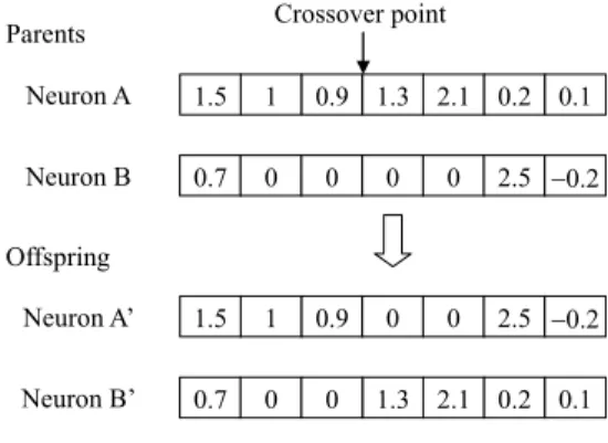
The structure and weights of the neurons are exchanged simultaneously through three steps. First, two parents are selected according to binary tournament selection [29]. Sec-ond, the crossover point is randomly selected, as shown in Fig. 6. Third, the components are exchanged starting from the crossover point to the end of the parents. Finally, two offspring (Neurons A0and B0) are generated.
FIGURE 6. Neuron crossover.
FIGURE 7. Neuron mutation.
2) NEURON MUTATION
Neuron mutation is performed on the connectivity and acti-vation function type of a neuron excepted for the output connection. The frequency of applying the neuron mutation operator is controlled by a mutation probability pm, which is a user-specified parameter. For each gene, a random number rwith a uniform distribution between 0 and 1 is generated. If r < pm, then the neuron mutation is performed on the gene. Three types of neuron mutations are presented in Fig. 7: the first shows the activation function type being modified from 0 (linear function) to 1 (hyperbolic tangent function), the second shows the connected weight being modified from −0.4 (connected) to 0 (disconnected), and the third shows the disconnected weight being modified from 0 (disconnected) to 2.9 (connected). Notably, the value of 2.9 is randomly assigned through normal distribution with a zero mean and unit variance after the weight is connected.
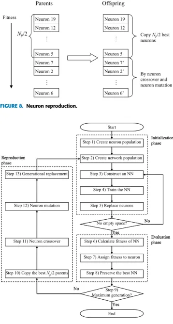
FIGURE 8. Neuron reproduction.
FIGURE 9. SSLA flowchart.
3) SURVIVAL SELECTION
In the reproduction phase, offspring are generated through three steps, as shown in Fig. 8. The first step is to rearrange the parents in descending order of fitness, the second step is to copy the best Np/2 parents as the offspring, and the third step is to generate the remaining Np/2 offspring through neuron crossover and mutation based on all of the parents. In the SSLA, generational replacement is adopted as the survival selection method; thus, the offspring replace all of the parents and then become parents themselves in the next generation. For example, Neuron 70 in Fig. 8 represents the offspring neuron that replaces Neuron 7 (although Neuron 70 is not generated from Neuron 7) and which is stored in the same memory as Neuron 7.
The major steps of the SSLA are outlined in Fig. 9, and can be summarized as follows:
Initialization phase:
Step 1) Create a neuron population consisting of Np neu-rons.
Step 2) Create a network population consisting of P groups with d empty spaces.
Step 3) Randomly select one group, Group p, to construct a NN in an empty space based on randomly selected pneurons from the neuron population.
Step 4) Train the NN by using the BP algorithm for ϕ
epochs.
Step 5) Replace the selected p neurons in the neuron pop-ulation with the trained p neurons. Return to Step 3 and repeat Steps 3–5 until each group in the network population has d NNs.
Evaluation phase:
Step 6) Calculate the fitness of the NN.
Step 7) Assign fitness values to the neurons in the neuron population through fitness sharing.
Step 8) Preserve the NN with the best fitness.
Step 9) If maximum generation is achieved, then terminate the algorithm; otherwise, continue to Step 10. Reproduction phase:
Step 10) Copy the best Np/2 parents as the offspring. Step 11) Generate the remaining Np/2 offspring through
neuron crossover based on the whole neuron popu-lation.
Step 12) Perform neuron mutation on the Np/2 offspring from Step 11.
Step 13) Perform the generational replacement and return to Step 2.
IV. EXPERIMENTAL RESULTS
This section provides three examples that verify the per-formance of the SSLA-derived FNAGM, called the FNAGM–SSLA, in real-time prediction applications.The first example predicts the chaotic time series. The second example predicts the object trajectory acquired from a vision-based robot. The third example predicts the lower limb motion for a rehabilitation system. The experiments were executed with an Intel Pentium CPU at 1.5 GHz with 512 MB RAM.
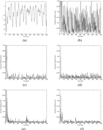
A. EXAMPLE 1: CHAOTIC TIME SERIES PREDICTION The Mackey–Glass system [30] is a benchmark system of time series prediction research, as shown in Fig. 10a. It gen-erates an irregular time series from the following delay dif-ferential equation:
dx(t)
dt =
0.2x(t − τ)
1 + x10(1 −τ)−0.1x(t) (5)
where τ = 25 and x(0) = 1.2 in the simulation. The
objective involves using [x(t − 3)x(t − 2)x(t − 1)x(t)] to predict x(t + 1). Thus, the input of the NN in the FNAGM is [eGM(t − 3)eGM(t − 2)eGM(t − 1)eGM(t)] and the output
as the training data for the structure learning of the FNAGM by the SSLA. The initial values ofµ and β are set at 0.001 and 4/3, respectively, in the FNAGM. The parameters of the SSLA are established as follows: probability of mutation (pm) = 0.1, neuron population size (Np) = 50, number of groups (P) = 5, number of group members (d ) = 3, and maximum number of generations (Gmax) = 250.
To compare the performance of the FNAGM–SSLA with other methods, the GM(1,1) [19], advanced GM(1,1) [31] and FNAGM [18] were implemented, where the advanced GM(1,1) adopted the Lagrange polynomial to further improve the GM(1,1), and the FNAGM was designed without the SSLA. Furthermore, a NN applied to forecasting time series [32] was implemented to identify the strengths and weaknesses of the FNAGM–SSLA. The NN adopted the first 250 input–output data pairs to train the weights offline, and then predicted the subsequent 750 input–output data pairs online. The number of hidden neurons of the FNAGM and NN were selected using a preliminary test, in which the performance of both was evaluated with 1–20 hidden neu-rons. The evaluation results showed that the FNAGM with four hidden neurons and the NN with seven hidden neurons exhibited the optimal performance; both the FNAGM and NN in this scenario possessed a fully connected topology.
FIGURE 10. (a) Mackey–Glass time series in Example 1 and the corresponding absolute prediction errors of (b) GM(1,1); (c) advanced GM(1,1); (d) NN; (e) FNAGM; (f) FNAGM–SSLA.
Fig. 10b–f show the absolute prediction errors of these methods. The FNAGM outperformed the GM(1,1), advanced
GM(1,1), and NN, whereas the FNAGM–SSLA further improved the FNAGM and had a smaller prediction error. Although the FNAGM–SSLA had a larger prediction error in the early time steps, it continually learned to predict and improve the prediction error.
TABLE 1.Comparison of prediction results for example 1.
To more clearly illustrate the efficiency of the proposed FNAGM–SSLA, Table 1 summarizes a comparison of the RMSE, number of hidden neurons (Nh), number of connec-tions (Nc), and computation time of each prediction step (Tc, in seconds) for all of the methods. The computation time was measured from reading new time series data until the one-step-ahead predictive value was determined. All results of the NN, FNAGM, and FNAGM–SSLA are the average of ten independent runs. In particular, the FNAGM–SSLA exhibited a smaller RMSE (6.92 × 10⁻⁴) than did the other methods. It also had a more compact structure than the FNAGM and NN in terms of Nhand Nc because of the use of the SSLA. This implies that more connections do not necessarily lead to superior prediction performance; the key to improving prediction ability is the appropriateness of the connected topology, rather than the number of connections. Because the FNAGM–SSLA had fewer connections (13.6 on aver-age) than the FNAGM (25) and NN (43), it required less computation time (1.90 × 10⁻³s on average) than did the
FNAGM (4.80 × 10⁻³ s) for both prediction and online
batch training. Although the FNAGM–SSLA required more computation time than did the NN (1.81 × 10⁻⁴s) for online batch training, it can be employed for real-time prediction applications where the sampling time is longer than 2 ms.
FIGURE 11. Evolved NN of the FNAGM–SSLA for Example 1.
Fig. 11 shows the evolved NN of the FNAGM, with the blue lines representing weights with positive values and the red lines representing weights with negative values. Notably, the width of the lines is proportional to the relative strength of the weight. The inputs u1, u2, u3, and u4represent eGM(t),
eGM(t − 1), eGM(t − 2), and eGM(t − 3), respectively.
Addi-tionally, the evolved NN consists of two hidden neurons with a hyperbolic tangent activation function and ten connections (of note, the bias does not connect to either hidden neuron). Furthermore, u3 connects to the right neuron while u1, u2,
and u4do not. This indicates that the evolved NN originally
consisted of a few hidden neurons with a linear activation function. According to the concept described in Section III-A, the evolved NN can be further simplified to an equivalent NN by transforming the hidden neurons with a linear activation function into weights connected between the inputs and the output neuron. Therefore, u1–u4directly connect to the output
neuron because of simplification. The SSLA’s emphasis on evolving neurons with linear and hyperbolic tangent acti-vation functions in the reproduction phase can reduce not only the network complexity but also the computation time; thus, the evolved NN is clearly a partially connected feedfor-ward NN.
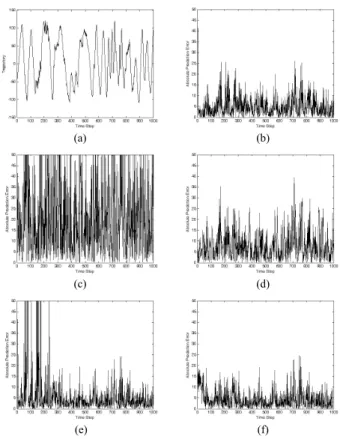
B. EXAMPLE 2: OBJECT TRAJECTORY PREDICTION A low sampling rate and high latency are inherent problems in most vision systems [33]. Thus, a robot must predict object trajectories in order to make adequate decisions for real-time human–robot interactions. To demonstrate the ability to solve a real problem, the FNAGM–SSLA was adopted to predict the object trajectory for a vision-based robot (described in detail in [34]). The movement of the object was generated according to an arbitrary pattern with varying velocity and a set level of noise. The movement was captured by the camera of the robot (30 frames per second) in an indoor environment and is shown in Fig. 12a. This experiment was designed to predict movement during one sampling interval (3.3×10⁻²s in this case), and the input–output data pair was obtained in the same format as that in Example 1 (which adopted the four
most recent data points as the input data and
the one-step-ahead value as the output data). The setup of the FNAGM–SSLA was identical to that in Example 1, and the input–output data were normalized within the range [−1, 1].
To evaluate the effectiveness of the proposed
FNAGM–SSLA, the GM(1,1), advanced GM(1,1), FNAGM, and NN were implemented, and the number of hidden neu-rons in the FNAGM and NN were selected following the same procedure used in Example 1. Consequently, the FNAGM with five hidden neurons and NN with four hidden neurons exhibited the optimal performance; notably, both possessed a fully connected topology. The training procedure of the NN was also identical to that for Example 1, and Fig. 12b–f show the absolute prediction errors of these methods. Notably, the GM(1,1) outperformed the advanced GM(1,1) and NN in this example, whereas the advanced GM(1,1) and NN outperformed the GM(1,1) in Example 1. Because the movement pattern was inconsistent over time, the GM(1,1) adjusted its parameters to handle the movement variations when online, whereas the NN did not. However, the FNAGM outperformed the GM(1,1) because of the application of the online batch training, and the FNAGM–SSLA further
FIGURE 12. (a) Object trajectory in Example 2 and the corresponding absolute prediction errors of (b) GM(1,1); (c) advanced GM(1,1); (d) NN; (e) FNAGM; (f) FNAGM–SSLA.
TABLE 2.Comparison of prediction results for example 2.
improved the prediction error of the FNAGM because of the evolved partially connected NN.
Table 2 compares all of the methods in terms of their RMSE, Nh, Nc, and Tcresults, which are the average of ten independent runs. In particular, the FNAGM–SSLA achieved a smaller RMSE (5.3806) than did the other methods. Further-more, the FNAGM–SSLA exhibited fewer hidden neurons (1.3) and connections (8.7) than did the NN and FNAGM. The SSLA was demonstrably more efficient at exploring the structure search space than was observed in the preliminary test, resulting in the construction of a partially connected NN with high prediction accuracy. Owing to its compact structure, the FNAGM–SSLA required less computation time (1.80 × 10⁻³s) than did the FNAGM for both prediction and online batch training. The experiments showed that partially connected NNs have greater storage capacity per connection than fully connected NNs in online prediction applications. Furthermore, it was confirmed that the FNAGM–SSLA can
FIGURE 13. Evolved NN of the FNAGM–SSLA for Example 2.
continuously adapt the NN to dynamic changes in movement for a real-time robot vision system.
Fig. 13 shows the evolved NN of the FNAGM–SSLA. This evolved NN consisted of one hidden neuron with a hyperbolic tangent activation function and eight connections. Notably, neither the bias nor the u2were connected to the hidden
neu-ron; however, the bias and four inputs were directly connected to the output neuron. The direct connection from the inputs to the output neuron is similar to that shown in Example 1. The evolved partially connected NN demonstrates that the appli-cation of the linear activation function in the reproduction phase is a crucial factor of the SSLA for evolving a compact topology.
FIGURE 14. IMU package for Example 3.
C. EXAMPLE 3: ANGULAR RATE PREDICTION
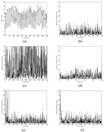
Acquisition of lower limb movement is key in many reha-bilitation systems. Relatedly, prediction of the lower limb movement is necessary when a wireless protocol is adopted to transmit the data of the lower limb movement, which may lead to a slow response and inaccurate decisions due to the low sampling rate. Fig. 14 shows an inertial measure-ment unit (IMU) package that includes inertial sensors and a wireless unit attached to a subject’s lower limb, which mea-sures the movement for a real-time rehabilitation application. Because the lower limb motion (i.e., gait pattern) is a periodic but irregular pattern, as shown in Fig. 15(a), an online adapta-tion of the predicadapta-tion model is required to deal with the time variant gait patterns. For this experiment, the FNAGM–SSLA was adopted to predict the lower limb motion (i.e., angular rate) for a rehabilitation system. The IMU package was devel-oped in the Mechanical System Control Laboratory at the
FIGURE 15. (a) Angular rate in Example 3 and the corresponding absolute prediction errors of (b) GM(1,1); (c) advanced GM(1,1); (d) NN;
(e) FNAGM; (f) FNAGM–SSLA.
TABLE 3.Comparison of prediction results for example 3.
University of California (Berkeley), where the sampling rate is 20 Hz. The four most recent data points were adopted as the input data and the one-step-ahead value was adopted as the output data. The setup of the FNAGM–SSLA was identical to that in Example 1.
Fig. 15b–f show the absolute prediction errors of all meth-ods. First, the FNAGM outperformed both the GM(1,1) and advanced GM(1,1). Notably, the NN performed better in the first 250 time steps (training data) than it did in the remaining 750 time steps (testing data). A slight difference between the training and testing data was observed, and was attributed to the irregular nature of subject’s gait patterns. However, although the FNAGM had a larger prediction error in the early time steps than did the NN, it was able to conduct continuous adaptation so that its prediction performance in the remaining 750 time steps was more accurate than the NN. The FNAGM–SSLA further improved the FNAGM, and it had an even smaller prediction error than did the FNAGM.
Table 3 compares all of the methods in terms of their RMSE, Nh, Nc, and Tc results, which are the average of ten independent runs. Notably, the FNAGM–SSLA achieved a smaller RMSE (3.6797) than did the other methods; this method also exhibited fewer hidden neurons (3.8) and con-nections (25.8) than did the NN and FNAGM. These results were attributed to the SSLA, which could obtain a FNAGM with a partially connected NN and thus ensure a higher prediction accuracy performance than that of a FNAGM with a fully connected NN. Furthermore, the FNAGM–SSLA required less computation time (3.85 × 10⁻³s) than did the FNAGM due to its compact structure. Although the com-putation time of the FNAGM–SSLA was longer than the GM(1,1), advanced GM(1,1), and NN, it was sufficient for the real-time application that had a sampling time of 0.05 s. Similar to the first two examples, this experiment showed that the FNAGM–SSLA can continuously adapt the NN to time variant gait patterns for a real-time rehabilitation system.
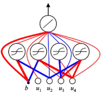
FIGURE 16. Evolved NN of the FNAGM–SSLA for Example 3.
Fig. 16 shows the evolved NN of the FNAGM–SSLA, which consists of four hidden neurons with hyperbolic tan-gent activation function and 19 connections. The u1 did
not connect to the hidden neurons, whereas the bias and four inputs were directly connected to the output neuron. This direct connection from the inputs to the output neuron was conducted by using the linear activation function of the SSLA, which facilitates a compact topology and short computation time.
V. CONCLUSIONS
This paper presented a novel forecasting system, the FNAGM–SSLA, which first facilitates the structure learning of an FNAGM by using the SSLA when offline and then achieves prediction and online batch training by applying the evolved FNAGM. The primary concepts underlying the SSLA are to evolve a set of neurons that cooperate well with each other, and to construct a partially connected NN from the neurons through symbiotic evolution. The SSLA shares the fitness of the NNs with the participating neurons and evolves the neurons through neuron crossover and mutation processes. Additionally, the SSLA emphasizes evolving neu-rons with linear and hyperbolic tangent activation functions in the reproduction phase, resulting in a compact network topology. Experiments were conducted to assess the perfor-mance of the FNAGM–SSLA in three real-time prediction
problems, relative to that of other methods. For all three problems, the FNAGM–SSLA was found to be the superior prediction model. The experimental results also demonstrated that applying the linear activation function triggers the evo-lution of direct connections from the inputs to the output neuron, thus reducing network complexity. Moreover, the FNAGM–SSLA has a more compact topology and smaller prediction error than does the FNAGM, which has an empir-ical design. In other words, the partially connected NNs possess more efficient information-processing capabilities per connection than fully connected NNs. This implies that an appropriately connected topology is the key to improv-ing prediction accuracy. Finally, the experiments revealed that the FNAGM–SSLA can continuously adapt NNs to the dynamic variation of time series by using online batch train-ing. Although the FNAGM–SSLA requires longer compu-tation time than the other methods (because of the online batch training), it remains feasible for real-time prediction applications.
REFERENCES
[1] E. M. Azoff, Neural Network Time Series Forecasting of Financial
Mar-kets. Hoboken, NJ, USA: Wiley, 1994.
[2] B. Kosko, Neural Networks and Fuzzy Systems: A Dynamical
Sys-tems Approach to Machine Intelligence. Upper Saddle River, NJ, USA: Prentice-Hall, 1992.
[3] P.-Y. Chou, J.-T. Tsai, and J.-H. Chou, ‘‘Modeling and optimizing tensile strength and yield point on a steel bar using an artificial neural network with Taguchi particle swarm optimizer,’’ IEEE Access, vol. 4, pp. 585–593, 2016.
[4] C. M. Bishop, Neural Networks for Pattern Recognition. London, U.K.: Oxford Univ. Press, 1995.
[5] M. M. Islam, M. A. Sattar, M. F. Amin, X. Yao, and K. Murase, ‘‘A new adaptive merging and growing algorithm for designing artificial neural networks,’’ IEEE Trans. Syst., Man, Cybern. B, Cybern., vol. 39, no. 3, pp. 705–722, Jun. 2009.
[6] S.-H. Yang and Y.-P. Chen, ‘‘An evolutionary constructive and pruning algorithm for artificial neural networks and its prediction applications,’’
Neurocomputing, vol. 86, pp. 140–149, Jun. 2012.
[7] M. M. Kordmahalleh, M. G. Sefidmazgi, and A. Homaifar, ‘‘A bilevel parameter tuning strategy of partially connected ANNs,’’ in Proc. IEEE
14th Int. Conf. Mach. Learn. Appl. (ICMLA), Dec. 2015, pp. 793–798. [8] J.-T. Tsai, J.-H. Chou, and T.-K. Liu, ‘‘Tuning the structure and parameters
of a neural network by using hybrid Taguchi-genetic algorithm,’’ IEEE
Trans. Neural Netw., vol. 17, no. 1, pp. 69–80, Jan. 2006.
[9] D. E. Moriarty and R. Miikkulainen, ‘‘Efficient reinforcement learning through symbiotic evolution,’’ Mach. Learn., vol. 22, no. 1, pp. 11–32, 1996.
[10] A. Canning and E. Gardner, ‘‘Partially connected models of neural net-works,’’ J. Phys. A, Math. Gen., vol. 21, no. 15, p. 3275, 1988.
[11] S. Kang and C. Isik, ‘‘Partially connected feedforward neural networks structured by input types,’’ IEEE Trans. Neural Netw., vol. 16, no. 1, pp. 175–184, Jan. 2005.
[12] K. O. Stanley and R. Miikkulainen, ‘‘Evolving neural networks through augmenting topologies,’’ Evol. Comput., vol. 10, no. 2, pp. 99–127, 2002. [13] D. Floreano, P. Dürr, and C. Mattiussi, ‘‘Neuroevolution: From
architec-tures to learning,’’ Evol. Intell., vol. 1, no. 1, pp. 47–62, Mar. 2008. [14] D. C. Park, M. A. El-Sharkawi, R. J. Marks, II, L. E. Atlas, and
M. J. Damborg, ‘‘Electric load forecasting using an artificial neural net-work,’’ IEEE Trans. Power Syst., vol. 6, no. 2, pp. 442–449, May 1991. [15] D. Saad, On-Line Learning in Neural Networks, vol. 17. Cambridge, U.K.:
Cambridge Univ. Press, 2009.
[16] C.-F. Juang and K.-J. Juang, ‘‘Circuit implementation of data-driven TSK-type interval TSK-type-2 neural fuzzy system with online parameter tuning ability,’’ IEEE Trans. Ind. Electron., vol. 64, no. 5, pp. 4266–4275, May 2017.
[17] Y.-H. Hsiao, ‘‘Household electricity demand forecast based on context information and user daily schedule analysis from meter data,’’ IEEE
Trans. Ind. Informat., vol. 11, no. 1, pp. 33–43, Feb. 2015.
[18] S.-H. Yang and Y.-P. Chen, ‘‘Intelligent forecasting system using Grey model combined with neural network,’’ Int. J. Fuzzy Syst., vol. 13, no. 1, pp. 8–15, 2011.
[19] J. L. Deng, ‘‘Introduction to grey system theory,’’ J. Grey Syst., vol. 1, no. 1, pp. 1–24, 1989.
[20] R. E. Smith, S. Forrest, and A. S. Perelson, ‘‘Searching for diverse, coop-erative populations with genetic algorithms,’’ Evol. Comput., vol. 1, no. 2, pp. 127–149, 1993.
[21] C.-F. Juang, J.-Y. Lin, and C.-T. Lin, ‘‘Genetic reinforcement learning through symbiotic evolution for fuzzy controller design,’’ IEEE Trans.
Syst., Man, Cybern. B, Cybern., vol. 30, no. 2, pp. 290–302, Apr. 2000. [22] C.-J. Lin and Y.-J. Xu, ‘‘A self-adaptive neural fuzzy network with
group-based symbiotic evolution and its prediction applications,’’ Fuzzy Sets
Syst., vol. 157, no. 8, pp. 1036–1056, 2006.
[23] C. J. Lin, C. H. Chen, and C. T. Lin, ‘‘Efficient self-evolving evolutionary learning for neurofuzzy inference systems,’’ IEEE Trans. Fuzzy Syst., vol. 16, no. 6, pp. 1476–1490, Dec. 2008.
[24] Y.-C. Hsu and S.-F. Lin, ‘‘Reinforcement group cooperation-based symbi-otic evolution for recurrent wavelet-based neuro-fuzzy systems,’’
Neuro-computing, vol. 72, pp. 2418–2432, Jun. 2009.
[25] Y.-C. Hsu, S.-F. Lin, and Y.-C. Cheng, ‘‘Multi groups cooperation based symbiotic evolution for TSK-type neuro-fuzzy systems design,’’ Expert
Syst. Appl., vol. 37, no. 7, pp. 5320–5330, 2010.
[26] Y.-P. Lin et al., ‘‘A battery-less, implantable neuro-electronic interface for studying the mechanisms of deep brain stimulation in rat models,’’ IEEE
Trans. Biomed. Circuits Syst., vol. 10, no. 1, pp. 98–112, Feb. 2016. [27] M. T. Hagan and M. B. Menhaj, ‘‘Training feedforward networks with
the Marquardt algorithm,’’ IEEE Trans. Neural Netw., vol. 5, no. 6, pp. 989–993, Nov. 1994.
[28] D. E. Rumelhart, G. E. Hinton, and R. J. Williams, ‘‘Learning repre-sentations by back-propagating errors,’’ Nature, vol. 323, pp. 533–536, Oct. 1986.
[29] A. Brindle, ‘‘Genetic algorithms for function optimization,’’ Doctoral the-sis, Univ. Alberta, Edmonton, AB, Canada, 1980.
[30] M. C. Mackey and L. Glass, ‘‘Oscillation and chaos in physiological control systems,’’ Science, vol. 197, no. 4300, pp. 287–289, 1977. [31] H.-C. Ting, J.-L. Chang, C.-H. Yeh, and Y.-P. Chen, ‘‘Discrete time
sliding-mode control design with grey predictor,’’ Int. J. Fuzzy Syst., vol. 9, no. 3, p. 179, 2007.
[32] M. Adya and F. Collopy, ‘‘How effective are neural networks at forecasting and prediction?’’ J. Forecasting, vol. 17, pp. 481–495, Sep./Nov. 1998. [33] P. I. Corke, ‘‘Dynamic issues in robot visual-servo systems,’’ in Robotics
Research. London, U.K.: Springer, 1996, pp. 488–498.
[34] S.-H. Yang, C.-Y. Ho, and Y.-P. Chen, ‘‘Neural network based stereo matching algorithm utilizing vertical disparity,’’ in Proc. 36th Annu. Conf.
IEEE Ind. Electron. Soc. (IECON), Nov. 2010, pp. 1155–1160.
SHIH-HUNG YANG received the B.S. degree in mechanical engineering, the M.S. degree in electri-cal and control engineering, and the Ph.D. degree in electrical and control engineering from National Chiao Tung University, Taiwan, in 2002, 2004, and 2011, respectively. Prior to joining the faculty, he was a Visiting Researcher with the University of California at Berkeley, Berkeley, USA, in 2012, and a Post-Doctoral Researcher with Academia Sinica, Taiwan, in 2013, where he developed fall prediction system. He is currently an Assistant Professor with the Depart-ment of Mechanical and Computer Aided Engineering, Feng Chia Univer-sity, Taiwan. His researches include neural networks and brain–machine interface.
WUN-JHU HUANG received the B.S. degree from the Department of Mechanical and Computer Aided Engineering, Feng Chia University, Taiwan, in 2013, where he is currently pursuing the M.S. degree. He is currently involved in developing neu-ral networks.
JIAN-FENG TSAI received the B.S. and M.S. degrees from National Tsing Hua University, Taiwan, and the Ph.D. degree in electrical and control engineering from Chiao Tung Univer-sity, Taiwan. He is currently an Assistant Pro-fessor with the Department of Electrical Engi-neering, National Formosa University, Taiwan. His researches include control theories, switching power converters, and motor drive.
YON-PING CHEN received the B.S. degree in electrical engineering from National Taiwan Uni-versity, Taiwan, in 1981, and the M.S. and Ph.D. degrees in electrical engineering from the Uni-versity of Texas at Arlington, USA, in 1986 and 1989, respectively. He is currently a Distinguished Professor with the Department of Electrical Engi-neering, National Chiao Tung University, Taiwan. His researches include control, image signal pro-cessing, and intelligent system design.