使用二級式 QuickRBF 及 Fuzzy ARTMAP 演算法於蛋白質二級結構預測

國 立 交 通 大 學

電 機 與 控 制 工 程 研 究 所

碩 士 論 文

使用二級式 QuickRBF 及 Fuzzy ARTMAP

演算法於蛋白質二級結構預測

Two-Stage QuickRBF and Fuzzy ARTMAP to

Protein Secondary Structure Prediction

研 究 生 ： 林 彥 宏

指 導 教 授： 張 志 永

使用二級式 QuickRBF 及 Fuzzy ARTMAP

演算法於蛋白質二級結構預測

Two-Stage QuickRBF and Fuzzy ARTMAP to

Protein Secondary Structure Prediction

學 生 : 林彥宏 Student : Yen-Hung Lin

指導教授 : 張志永 Advisor : Jyh-Yeong Chang

國立交通大學

電機與控制工程學系

碩士論文

A Thesis

Submitted to Department of Electrical and Control Engineering

College of Electrical Engineering and Computer Science

National Chiao Tung University

in Partial Fulfillment of the Requirements

for the Degree of Master in

Electrical and Control Engineering

June 2006

Hsinchu, Taiwan, Republic of China

使用二級式 QuickRBF 及 Fuzzy ARTMAP

演算法於蛋白質二級結構預測

學生：林彥宏 指導教授：張志永博士 國立交通大學電機與控制工程研究所

摘要

隨著人類基因定序及許多基因定序計畫陸續完成，序列的資料量將大幅成 長，有效地分析這些序列更顯得重要了。基於物運作的原則（Central Dogma）， 蛋白質的功能與結構遂成為相當重要的研究議題，而目前在蛋白質相關問題的解 決上，科學家都是利用X光繞射以及核磁共振 (NMR) 來取得實驗結果。這些方 法雖然正確率高，但是相對地所要花費的時間及成本是相當高的。因此，研究人 員便利用電腦科學來協助解決這些問題，相信是能夠有效降低實驗成本的。由於 要了解完整蛋白質的功能必需從三級結構著手，但直接從蛋白質序列去預測它的 三級結構是非常困難的議題，因此一個間接且有助益的方式，便是預測其二級結 構。過去的研究中，學者們通常將蛋白質二級結構分成三種類別，分別是螺旋體 （helix）、摺疊（sheet）、其他部份歸類為迴圈（loop）。因此我們可以將蛋白質 二級結構預測視為一個普遍的分類問題 本篇論文中，我們提出利用二層快速徑向基底函數網路分類器（Quick Radial Basis Function）來預測蛋白質二級結構。快速徑向基底函數網路分類器能夠迅速 地建構分類器的模型，其預測準確性更是不亞於目前廣受歡迎的機器學習演算法 支持向量機（Support Vector Machine）。最後，將各層分類之結果合併，而有效 的提高預測之準確度。在本研究中，我們使用著名的 RS126 資料集，以及 PSI- BLAST 所產生的 PSSM，所達到的最佳準確率為76.7%。

Two-Stage QuickRBF and Fuzzy ARTMAP to

Protein Secondary Structure Prediction

STUDENT: YEN-HUNG LIN ADVISOR: JYH-YEONG CHANG

Institute of Electrical and Control Engineering National Chiao-Tung University

ABSTRACT

The majority of human coding regions have been sequenced and several genome sequencing projects have been completed. With the growth of large-scale sequencing data, an efficient approach to analyze protein is more important since protein function and structures are crucial issues in bioinformatics. Nowadays, scientists use X-ray diffraction or nuclear magnetic resonance (NMR) to solve the protein structure problems. Even though chemical experiments can achieve high accuracy, they in the mean time incur high cost and long time to solve the protein problems. Hence, computational tools are then applied thereto and considered as promising ways which not only reduce the time and the cost but also maintain reliable predictive results. The protein secondary prediction (PSS) is an intermediate but useful step for the three-dimensional (tertiary) structure prediction. In the previous work, researchers always focused on classifying three states of protein secondary structure: helix, strand and coil classes. It is a common classification problem for the prediction of protein secondary structure.

In this thesis, a high-performance method was developed for protein secondary structure prediction based on the dual-layer QuickRBF technology that has been

successfully applied in solving problems in the field of bioinformatics. The QuickRBF is capable of delivering the same level of performance as the state of art approach, SVM, while having execution efficiency during the phase to construct the classifier. The performance was further improved by combining PSSM profiles with the QuickRBF analysis where the PSSMs were generated from PSI-BLAST profiles, which contain important evolution information. The final prediction results were generated from the first fusion method. We report a maximum prediction accuracy of 76.7% on the famous RS126 dataset based on the PSI-BLAST profiles.

ACKNOWLEDGEMENT

I would like to express my sincere appreciation to my advisor, Dr. Jyh-Yeong Chang. Without his patient guidance and inspiration during the two years, it is impossible for me to overcome the obstacles and complete the thesis. In addition, I am thankful to all my lab members for their discussion and suggestion.

Finally, I would like to express my deepest gratitude to my parents. Without their fully support and encouragement, I could not go through these two years.

Content

ABSTRACT (CHINESE)……….i

ABSTRACT (ENGLISH)...………ii

ACKNOWLEDGEMENT.…………...………...iii

Chapter 1. Introduction………...

1

1.1 Motivation and the Background of This Research………1

1.2 Introduction to the Protein Secondary Structure………...…...2

1.3 Introduction to Neural Networks and Approximation Schemes……...……..7

1.4 Thesis Outline………...10

Chapter 2. Quick Radial Basis Functions………...…..11

2.1 Radial Basis Functions and QuickRBF………..………11

2.2 Fuzzy ART and Fuzzy ARTMAP…..………...16

2.2.1 Fuzzy ART ………...………...17

2.2.2 Fuzzy ARTMAP…..……….………...22

Chapter 3. Protein Secondary Structure Prediction………...26

3.2 A dual-layer SVM approach………..………….27

3.3 Quick Radial Basis Function……….…………30

3.4 A cascade of Fuzzy ARTMAP and QuickRBF approach………31

3.5 A dual-layer QuickRBF approach………..……...…34

3.6 Fusion Method………36

3.6.1 Reliability Index……….…36

3.6.2 Linear Combination and Weighted Sum Fusion.………38

Chapter 4. Experiment and Results……….………..40

4.1 Datasets………..………40

4.2 Results………41

4.2.1 Results of the Cascade of Fuzzy ARTMAP and QuickRBF………41

4.2.2 Results of the Dual-Layer QuickRBF and Fusion Methods………..……42

Chapter 5. Conclusion………46

List of Figures

Fig. 1.1. The α-helix structure…...………..…..4

Fig. 1.2. The Ramachandarn Plot………...…………...4

Fig. 1.3. The Anti-parallel β-sheet……..………...5

Fig. 1.4. The Parallel β-sheet……….……….……….…6

Fig. 1.5. Two hairpin loops between three anti-parallel β-strands ……….6

Fig. 1.6. Approximation functions with different estimators.………...9

Fig. 2.1. General architecture of radial basis function networks………13

Fig. 2.2. Comparison of ART1 and fuzzy ART………..…21

Fig. 2.3. Geometric interpretation of Fuzzy ART.………..21

Fig. 2.4. Fuzzy ARTMAP architecture………….………..25

Fig. 3.1. The dual-layer SVM architecture………..…………...29

Fig. 3.2. Geometry mean of hyperbox R ………..………...32 _j Fig. 3.3. The cascade of fuzzy ARTMAP and QuickRBF architecture.…………33

Fig. 3.4. The dual-layer QuickRBF architecture……...………35

Fig. 3.5. The accuracy distribution on different Reliability indices………..37

List of Tables

Table 3.1. Comparison of classification accuracy of the RS126 data set with

PSI-BLAST PSSM profiles………..30

Table 3.2. Fusion method 2: Linear combination………..39

Table 3.3. Fusion method 3: Weighted Sum………..………...39

Table 4.1. The seven fold of RS126……….………….41

Table 4.2. Single QuickRBF and cascade of FARTMAP and QuickRBF………42

Table 4.3. Results of different fusion method with 5000 centers at first stage..…44 Table 4.4. Results of different fusion method with 10000 centers at first stage….44 Table 4.5. Results comparison of several methods obtained on RS126 dataset….45

Chapter 1. Introduction

1.1 Motivation and the Background of This Research

The number of known proteins and its structure has been increased in recent

years. Since protein applications are more widely used, there will be a lot of problems to be solved. Nowadays, scientists use X-ray diffraction or nuclear magnetic resonance (NMR) to solve the protein structure problems, because protein structures are closed related to their functions. Even though chemical experiments can achieve high accuracy, they in the mean time incur high costs and long time to solve the protein problems. Hence, computational tools are then applied thereto and considered as promising ways which not only reduce the time and the costs but also maintain reliable predictive results. This motivation is triggered by the basic hypothesis that the three-dimensional (tertiary) structure of a protein is uniquely determined by its sequence of amino acids. Therefore, predicting protein structure from amino acid sequences becomes one of the most important issues in molecular biology.

The protein secondary prediction (PSS) is an intermediate and useful step for the three-dimensional (tertiary) structure prediction. To better predict secondary structure, many computational techniques have been proposed in the literature to solve the PSS prediction problem, for example: PHD, a novel prediction method proposed by Rost and Sander which uses evolutionary information and has obtained significant improvements [1]–[3]; SVM, a new method introduced by Hua and Sun which is based on statistical learning theory (SLT) [4]; and QuickRBF, a fast and innovative method proposed by Ou et al. [5] which is capable of delivering the same level of prediction accuracy as the LIBSVM proposed by Lin et al. [6], while having

execution efficiency during the phase to construct the classifier.

Despite the existence of many approaches, this issue still remains to be further studied. We propose that the single-stage approaches are unable to find complex relations (correlations) among different elements in the sequence. The result of incorporating second stage could be improved by incorporating the interactions or contextual information among the output elements of the secondary structures prediction, which are considerably reduced in their complexity. We believe it is feasible to enhance present single-stage approaches by cascading and fusing with another prediction scheme at their outputs and propose to use RBFN as the second-stage.

This thesis investigates the use of Radial Basis Function Networks for PSS prediction. We establish the QuickRBF technique based on multi-classifier to PSS prediction. Moreover, we cascade two multi-class QuickRBFs for the prediction scheme to improve the prediction accuracy from the output of the first stage. Finally, different fusion methods are applied and a high level of accuracy was achieved. We report a prediction accuracy of 76.7% on RS126 dataset based on PSI-BLAST profiles.

1.2 Introduction to the Protein Secondary Structure

Protein secondary structure prediction is to predict protein secondary structure based only on its sequence, where each amino acid is assigned a structure state, helix (H), strand (E) or coil (C). The secondary structure we used is assigned from the experimentally determined tertiary structure by the benchmark secondary structure definition, DSSP. According to DSSP, 8 types of protein secondary structure elements

were classified and denoted by letters: H (α-helix), E (extended β-strand), G (3 -helix), I (π-helix), B (isolated β-strand), T (turn), S (bend) and “_＂(rest). The ₁₀ 8 classes are usually reduced to three states of helix (H), sheet (E) and coil (C) by using one of the following methods:

1. H,G and I to H; E to E; all other states to C 2. H,G to H; E,B to E; all other states to C 3. H,G to H; E to E; all other states to C 4. H to H; E,B to E; all other states to C 5. H to H; E to E; all other states to C

The 8- to 3-state reduction method can alter the apparent prediction accuracy [6]. Although we can expect an accuracy increase by using method 5, we used the first method which is adopted by HYPROSP [8], [9].

The traditional three classes: α-helix, β-sheet and loop (coil) representing all the rest. The α-helix (Fig. 1.1) is the classic element of protein structure which is predicted to be stable and energetically favorable in proteins. Alpha helices in proteins are found when a stretch of consecutive residues all have the phi, psi angle pair approximately -85° and -50°, corresponding to the allowed region in the bottom left quadrant of the Ramachandran plot (Fig. 1.2).

Fig. 1.1. The α-helix structure.

Fig. 1.2. The Ramachandran plot.

-180° Φ(phi) 180° 180°

Ψ (psi)

Only in the α-helix are the backbone atoms properly packed to provide a stable structure. In globular proteins, the average length for α-helices is around ten residues, corresponding to three turns. The rise per residue of an α-helix is 1.5 Å along the helical axis, which corresponds to about 15 Å from one end to the other of an average α-helix.

The second major structural element found in globular proteins is the β-sheet. This structure is built up from a combination of several regions of the polypeptide chain, in contrast to the α-helix, which is built up from one continuous region. These regions, β-strands, are usually from five to ten residues long and are in an almost fully extended conformation with phi, psi angles within the broad structurally allowed region in the upper left quadrant of the Ramachandran plot (Fig. 1.2). The β-strands can interact in two ways to form a pleated sheet – parallel and anti-parallel. Each of the two forms has a distinctive pattern of hydrogen-bonding. The anti-parallel β-sheet (Fig. 1.3) has narrowly spaced hydrogen bond pairs that alternate with widely spaced pairs. Parallel β-sheets (Fig. 1.4) have evenly spaced hydrogen bonds that bridge the β-strands at an angle.

Fig. 1.4. The Parallel β-sheet.

Most protein structures are built up from combinations of secondary structure elements, α-helices and β-strands, which are connected by loop regions of various lengths and irregular shape. The loop regions are always at the surface of protein molecules. Loop regions exposed to solvent are rich in charge and polar hydrophilic residues. Loop regions that connect two adjacent anti-parallel β-strands are called the

hairpin loops. Short hairpin loops are usually called reverse turns or simply turns.

Fig. 1.5. Two hairpin loops between three anti-parallel β-strands.

1.3 Introduction to Neural Networks and Approximation Schemes

The problem of learning a mapping between an input and an output space is essentially equivalent to the problem of synthesizing an associative memory that retrieves the appropriate output when presented with the input and generalizes when presented with new inputs. It is also equivalent to the problem of estimating the system that transforms inputs into outputs given a set of examples of input-output pairs. A classical framework for this problem is Approximation Theory. Almost all approximation schemes can be mapped into some kind of network that can be dubbed as a “neural network.” Networks, after all, can be regarded as a graphic notation for a large class of algorithms. In the context of this thesis, a network is a function represented by the composition of many basic functions.

To measure the quality of the approximation, one introduces a distance function ρto determine the distance ρ[f(X), F(W, X)] of an approximation F(W, X) from f(X). The distance is usually induced by a norm, for instance the standard L ₂

norm. The approximation problem can be then stated formally as:

Approximation problem: If f(X) is a continuous function defined on set X, and

F(W, X) is an approximating function that depends continuously on W∈ and X, P

the approximation problem is to determine the parameters W* such that

ρ[F(W*, X), f(X)] <ρ [F(W, X), f(X)] (1.1)

for all W in the set P.

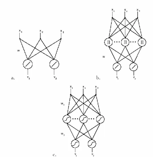
With these definitions we can consider a few examples of F(W, X), shown in

the Fig. 1.6 where (a) indicates a linear approximating function, (b) indicates polynomial estimators and other linear combinations of nonlinear features on the input, and (c) indicates a back-propagation network.

F(W, X) = WX (1.2)

where W is an m × n matrix and X is an n-dimensional vector. It

corresponds to a network without hidden units;

2) The classical approximation scheme is linear in a suitable basis of functions )

(X

i

Φ of the original inputs X, that is

F(W, X) = WΦ_i(X ) (1.3) and corresponds to a network with one layer of hidden units. Spline interpolation and many approximation schemes, such as expansions in series of orthogonal polynomials, are included in this representation. When theΦ are products and powers of the input components_i X , F is a _i

polynomial.

3) The nested sigmoids scheme (usually called back-propagation, BP in short) can be written as )...))) ( (... ( ( ) ( n n

∑

∑

∑

= i j j j i F W,X ρ w ρ ν ρ ρ u X (1.4)

and corresponds to a multilayer network of units that sum their inputs with “weights” w, v, u,… and then perform a sigmoidal transformation of this

sum. This scheme (of nested nonlinear functions) is unusual in the classical theory of the approximation of continuous functions.

In general, each approximation scheme has some specific algorithm for finding the optimal set of parameters W. An approach that works in general, though it may

not be the most efficient in any specific case, is some relaxation method, such as gradient descent or conjugate gradient or simulated annealing, in parameter space, attempting to minimize the error ρ over the set of examples. In any case, our discussion suggests that networks of the type used recently for simple learning tasks

applied networks of the type is an efficient construction of Radial Basis Function Networks used for fast modeling tasks and can be considered as specific methods of function approximation.

1.4 Thesis Outline

The organization of this thesis is structured as follows. Chapter 1 introduces the role of neural networks and the motivation and the background of this thesis. In Chapter 2, the quick radial basis function networks will be described. Moreover, we will present the fuzzy ARTMAP which was applied to a cascade of fuzzy ARTMAP and QuickRBF architecture detailed in the next chapter. We then will introduce the benchmark SVM approaches, and our paralleling QuickRBF architectures using different fusion methods in Chapter 3. In Chapter 4, the experiment of computer simulation and the results are conducted and compared to other prevailing methods, such as single stage SVM approach, dual-SVM approach and the famous PHD. Finally, the conclusion and future work of this thesis are presented in Chapter 5.

Chapter 2. Quick Radial Basis Functions

2.1 Radial Basis Functions and QuickRBF

Networks based on radial basis functions have been developed to address some of the problems encountered with training multilayer perceptrons: radial basis functions are usually able to converge and the training is much more rapid. Both are feed-forward networks with similar-looking diagrams and their applications are similar; however, the principles of action of radial basis function networks and the way they are trained are quite different from multilayer perceptrons.

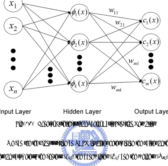
An RBFN (radial basis function network) consists of three layers, namely the input layer, the hidden layer and the output layer. The input layer broadcasts the coordinates of the input vector to each of the nodes in the hidden layer. Each node in the hidden layer then produces an activation based on the associated radial basis function. Finally, each node in the output layer computes a linear combination of the activations of the hidden nodes.

For radial basis function networks, each hidden unit represents the center of a cluster in the data space. Input to a hidden unit in a radial basis function is not the weighted sum of its inputs but a distance measure: a measure of how far the input vector is from the center of the basis function for that hidden unit. Various distance measures are used, but perhaps the most common is the well-known Eculidean distance measure.

If x andµare vectors, the Eculidean distance between them is given by

∑

− = − = i i i x D ₍

_µ

₎2 µ x (2.1)

node j. The hidden node then computes its outputs as a function of the distance between the input vector and its center. For the Gaussian radial basis function the hidden unit output is

2 2 2₎ /2 ( j σ j j D D h =

e

− (2.2)

whereD is the Euclidean distance between an input vector and the location vector _j

for hidden unit j; h is the output of hidden j and _j σ is a measure of the size of the

cluster j (in statistical terms it is called the variance or the square of the standard

deviation).

How an RBFN reacts to a given input stimulus is completely determined by the activation functions associated with the hidden nodes and the weights associated with the links between the hidden layer and the output layer. The general mathematical form of the output nodes in an RBFN is as follows:

∑

(

)

= − = k i ji i i i j w x c 1 ; ) (x

φ

µ

σ

(2.3)

where cj(x) is the function corresponding to the j-th output unit (class j) and is a

linear combination of k radial basis function φ (⋅) with centerµi and bandwidthσi.

Also, w is the weight vector of class j and j w is the weight corresponding to the ji

j-th class and i-th center. The general architecture of RBFN is shown as follows.

j j

Fig. 2.1. General Architecture of Radial Basis Function Networks.

We can see that constructing an RBFN involves determining the values of three sets of parameters: the centers (µi), the bandwidths (σi) and the weights (w ), in ji

order to minimize a suitable cost function.

In QuickRBF package, the centers are randomly selected and bandwidth are fixed and set as 5 for each kernel function for conducting the simplest method. The transformation between the inputs and the corresponding outputs of the hidden units is now fixed. The network can thus be viewed as an equivalent single-layer network with linear output units. Then, the LMSE method is used to determine the weights associated with the links between the hidden layer and the output layer.

Assume h is the output of the hidden layer.

h=

[

φ

₁(x),

φ

₂(x ) ,_K,

φ

_k(x)

]

T (2.4) where k is the number of centers, φ₁(x) is the output value of first kernel function

with input x. Then, the discriminant function c_j

( )

x of class j can be expressed by the following:

c_j(x)=wT_jh, j =1 ,2,_K ,m (2.5) where m is the number of class, and w is the weight vector of class j. We can show _j

j

w as:

w_j =

[

w_j1(x), w_j2(x ) ,_K, w_jk(x)

]

T (2.6) After calculating the discriminant function value of each class, we choose the class with the biggest discriminant function value as the classification result. We will discuss how to get the weight vectors by using least mean square error method in the following.

For a classification problem with m classes, let V designate the i-th column _i

vector of an m × m identity matrix and W be an k × m matrix of weights:

W =

[

w₁, w₂ ,_K ,w_m

]

(2.7) Then the objective function to be minimized

( )

{

}

1 2

∑

= − = m j j T j jE P J W W h V (2.8)

where P and _j E_j{⋅} are the a priori probability and the expected value of class j, respectively.

To find the optimal W that minimizes J, the gradient of J(W) is set to be zero: ( ) 2

{ }

2

{ }

jT [ ] 1 1 T _{W h V 0} hh w = − = ∇

∑

∑

= = m j j j m j j j wJ PE P E (2.9)

where [0] is a k × m null matrix. Let K denote the class-conditional matrix of the _i

{ }

_hhT

i

i E

K = (2.10) If K denotes the matrix of the second-order moments under the mixture distribution, we have

∑

= = m j j j P 1 K K (2.11)

Then Eq. (2.9) becomes

KW=M (2.12) where

{ }

1 T

∑

= = m j j j jE P h V M (2.13)

If K is nonsingular, the optimal W can be calculated by

W* ₌K-1M _(2.14)

However, there is a critical drawback of this method. That is, K may be singular and this will crash the whole procedure. By observing the matrix _{hh , we are aware} T of that the matrix _{hh is symmetric positive semi-definite (PSD) matrix with rank} T equal to 1. Since K is the summation of _{hh for each training instance, K is also a} T PSD matrix with rank smaller than n. However, PSD matrix may be a singular matrix, so we should add the regularization term to make sure the matrix will be invertible. In the regularization theory, it consists in replacing the objective function as follows:

{

}

j j m j m j j j jE P J W W h V wTw 1 1 2 T ) (

∑

∑

= = + − =

λ

(2.15)

where λ is the regularization parameter. Then the Eq. (2.12) becomes

(

K+λI

)

W=M (2.16) If we set λ >0,

(

K+λI

)

will be a positive definite (PD) matrix and therefore is nonsingular.The optimal _W* _{can be calculated by}

W* ₌

(

K_+λI

)

-1M _(2.17)

However, the PD matrix has many good properties, and one of them is a special and efficient triangular decomposition, Cholesky decomposition. By using Cholesky decomposition, we can decompose the

(

K+λI

)

matrix as follows:

(

K+λI

)

=LLT (2.18) where L is a lower triangular matrix. Then, the Eq. (2.16) becomes

(

LLT

)

W=M _(2.19)

Actually, the linear system can be solved efficiently by using back-substitution twice. Finally, we can get the optimal *

j

W for class j from _{W , and then the optimal} * discriminant function c_j(x) for class j is derived. By using the regularization theory, the optimal weights can be obtained analytically and efficiently.

2.2 Fuzzy ART and Fuzzy ARTMAP

The aim of classification, or cluster analysis, is to organize observations into similar groups. Cluster analysis is a commonly used, appealing and conceptually intuitive statistical method. Some of its uses include pattern recognition, where pixels of obtained images are grouped into clusters with similar attributes for targeted objects; gene expression analysis, where genes with similar expression patterns are grouped together and so on. A cluster analysis results in a simplification of a data set for two reasons: first, because each cluster, which is now relatively homogeneous, can be analyzed separately, and second, because the data set can be summarized by a description of each cluster. Thus, it can be used to effectively reduce the size of massive amounts of data. In this thesis, a famous tool of cluster discovery, fuzzy ARTMAP, is adopted to retrieve certain features existing in the dataset, and detailed

as follows.

2.2.1 Fuzzy ART

The Fuzzy ART architecture is capable of performing unsupervised learning against either binary or analog input vectors. Basically, Fuzzy ART consists of three neural layers: preprocessing F , matching ₀ F₁ and competitive F₂.

Every input vector component, a , must be normalized between 0 and 1. Layer _i

0

F is formed by 2M neurons, with M being the dimension of the input vectors, and

provides the complement code of the input vectors according to the following expression: = i I M i M M i M i i 2 1 1 1 ≤ ≤ + − ≤ ≤ − a a (2.20) Layer F₁ is also formed by 2M neurons and its function is to verify the match between input patterns and prototypes learned by the network. Finally, layer F₂ is a competitive layer. It works as a content addressable memory (Carpenter et al., 1998) where each neuron stores a prototype of a class of input vectors. F₂ is formed by a total number of N neurons which are recruited dynamically as they are needed to encode new classes of incoming vectors. Each layer is connected to the next through a set of adaptive weighted paths. These weights, W , form the long term memory _ij

(LTM) element of the neural network and evolve during the training phase. Every weight is initialized to 1 at the beginning of the training and monotonically decreases as the training proceeds and patterns are learned. This monotonical decrease of weights guarantees the eventual stability of the network.

Unsupervised learning in Fuzzy ART is performed in the following way. Each input pattern, a, is put into its complement code, I, according to Eq. (2.20), and then

it is transmitted through F₁ to layer F₂. Each neuron j in F₂ receives an activation, )

(I

j

T , that is a function of the input pattern and the LTM weights:

N j T j j j =1,K, + ∧ = W W I α (2.21)

where W_j =

[

W_j1 ,W_j2 ,_K ,W_j2M

]

are the weights associated with neuron j; ⋅ is the _{L norm,} 1

∑

= = M i i x 1

x ; x∧y =min{ yx, } is the fuzzy AND operator, for vectors, }x∧y =v with v=min{x,y and α∈ ,

[ ]

0 ∞ is a choice parameter

(typically α ≈ 0+).

At this point, the neurons in F₂ hold a WTA competition to select which neuron, J; is going to learn the pattern:

{ }

j j

T

J =argmax (2.22) After the competition, only the output of the winning neuron remains set to 1 and descends through the top-down weighted paths so that the prototype of neuron J is presented in layer F₁. In F₁ the matching between the input pattern, I; and the winner prototype, W , is evaluated according to a criterion determined by a user defined _j

parameter ρ∈

[ ]

0 ,1. The criterion is applied as follows:

1) If ∧ ≥ρ

I W

I _J

, then the input is considered to belong to match prototype in J and pattern is learn by neuron J.

2) If ∧ <ρ

I W

I _J

, then the system is reset and neuron J is inhibited so that it no longer enters the competition for the current pattern. In addition to this, a match tracking mechanism raises the value of parameter ρ so that the next winner must be closer to the pattern. After this new competition,

another winner is selected. Eventually, a new neuron in F₂ will be committed if none of the current neurons is found to match the pattern sufficiently.

When a winner successfully passes the matching criterion, learning occurs. LTM weights are updated according to the following learning law:

(

Old

)

(

)

Old New ₁ J J J W I W W =β ∧ + −β (2.23) where β∈

[ ]

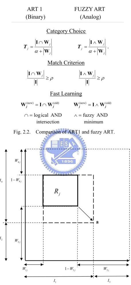
0 ,1 is the learning rate: β → 0+ implies slow learning, while β=1 implies fast learning and each pattern is incorporated to the knowledge stored by the network in just one iteration.

With complement coding of patterns and the _{L norm, each} 1 2

F neuron can be represented geometrically as a hyperbox in _{R covering all the patterns that it has} M

already learned. The size of the hyperbox R associated with neuron j, is determined _j

by weights W as showed in Fig. 2.2. Competition in layer _j F₂ has also a geometric interpretation. Activation function, T , is a measure of the distance between the _j

pattern a and R (Fig. 2.2). Therefore, the neuron with the box lying nearest to the _j

pattern will receive the highest activation. Parameter α in Eq. (2.21) is used to break ties when several boxes include the pattern; in such case, the smaller the box is, the higher the activation received.

Finally, the learning process can be viewed as the expansion of the winner neuron box toward the pattern. If fast learning is applied, the box grows until it actually covers the pattern, while under slow learning the box just expands toward the pattern but without covering it.

Referring to Fig. 2.2, it shows the geometric interpretation of Fuzzy ART. Box

j

input pattern a. Size of box R is determined by weighs associated with neuron j, _j

[

j j j j

]

j = W1 ,W2 ,W3 ,W4

W . In a generic M dimensions case, R size on dimension I _j

Fig. 2.2. Comparison of ART1 and fuzzy ART.

a

Fig. 2.3. Geometric interpretation of Fuzzy ART.

ART 1 FUZZY ART

(Binary) (Analog)

Category Choice

j j j j j j W W I W W I + ∧ = + ∩ = α α T T

.

Match Criterion

ρ ρ ∧ ≥ ≥ ∩ I W I I W I _{j j}

Fast Learning

(old) (new) (old) (new) j j j j I W W I W W = ∩ = ∧ AND fuzzy AND ical log ∧= = ∩ intersection minimum j W3 j W4 j W1 1−W3j j W2 j

R

j W4 1− 3 I 1 I 2 I 4 I

2.2.2 Fuzzy ARTMAP

Fuzzy ARTMAP is an incremental supervised learning of recognition categories and multidimensional maps in response to arbitrary sequences of analog or binary input vectors, which may represent fuzzy or crisp sets of features. It realizes a new minimax learning rule that conjointly minimizes predictive error and maximizes code compression, or generalization. It automatically learns a minimal number of recognition categories, or hidden units, which is achieved by a match tracking process.

The applications of ARTMAP involve analog patterns that are not necessarily interpreted as fuzzy set, but serve to illustrate the properties of the system and allow comparison with several existing systems, such as the benchmark back-propagation and genetic algorithm systems. In all cases, fuzzy ARTMAP simulations lead to favorable levels of learned predictive accuracy, speed, and code compression in both on-line and off-line setting [11].

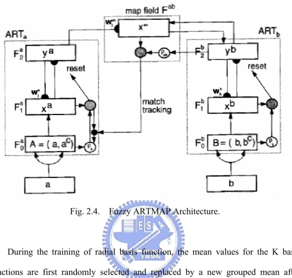
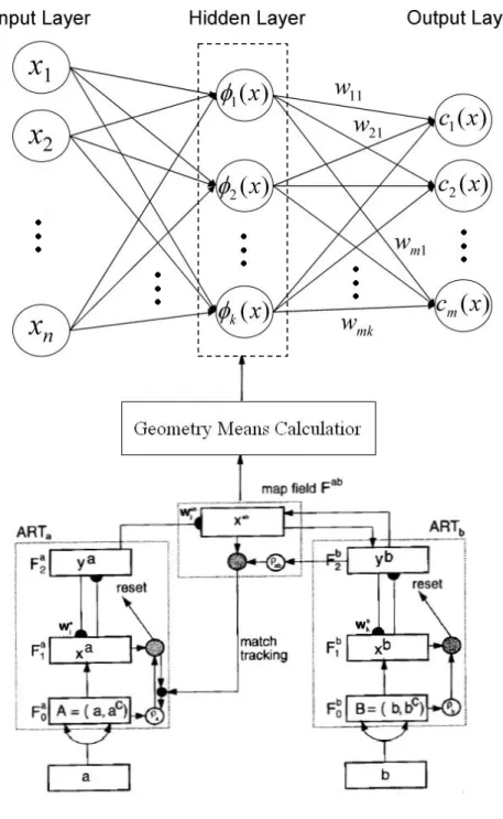
The fuzzy ARTMAP system incorporates two fuzzy ART modules, b

a andART

ART , that are linked together via an inter-ART module, _{F , called a} ab

map field. The map field is used to form predictive associations between categories

and to realize the match tracking rule, whereby the vigilance parameter of ART _a increases in response to a predictive mismatch at ART . Match tracking reorganizes _b category structure so that predictive error is not repeated on subsequent presentations of the input. The interactions mediated by the map field _{F may be operationally} ab

characterized as follows.

b a and ART

ART : Inputs to ART_a andART_b are in the complement code form: for

a

ART or ART are designated by subscripts or superscripts _b a and b. For ART , let _a

[

a

]

M a a a a x x x₁ , ₂,_L , ₂ ≡ x denote the _Fa

1 output vector; let ya ≡

[

y1a ,y2a ,L ,yNaa

]

denote the _Fa

2 output vector; and let waj ≡

[

waj1 ,waj2,L,waj,2Ma

]

denote the j-th a

ART weight vector. For ART , let _b

[

b

]

M b b b b x x x₁ , ₂ ,_L , ₂ ≡ x denote the _Fb 1 output vector; let

[

b

]

N b b b b y y y₁ , ₂ ,_L , ≡ y denote the _Fb

2 output vector; and let

[

b

]

M k b k b k b k ≡ w1 ,w 2,L,w ,2 b

w denote the k-th ART weight vector. For the map field, _b

let

[

ab

]

N ab ab ab b x x x₁ , ₂ ,_L , ≡

x denote the F_ab output vector; and let

[

ab

]

N j ab j ab j ab j ≡ w1 ,w 2,L,w , b

w denote the weight vector from the jth _Fa

2 node to Fab. Vectors _xa_{, y}a_{, x}b_{, y}b_{, andx}ab _{are set to 0 during input presentations.}

Map Field Activation: The map field _Fab _{is activated whenever one of the}

a ART or ART categories is active. If node _b J of _Fa

2 is chosen, then its weights wabj

activate _Fab _{If node K in F}b

2 is active, then the node K in Fab is activated by 1 to 1 pathways between _Fb

2 and Fab If both ARTa andARTb are active, then

ab

F becomes active only if ART predicts the same category as _a ART via the _b weights ab

j

w . The _Fab _{output vector x}ab _obeys

ab x = 0 y w w y b ab J ab J b _∧ inactive is and inactive is if active is and inactive is if inactive is and active is node th the if active is and active is node th the if 2 2 2 2 2 2 2 2 b a b a b a b a F F F F F F J F F J (2.24)

By Eq. (2.24), xab =0 _{if the prediction} ab j

w is disconfirmed by _{y . Such a} b

mismatch event triggers an ART search for a better category, as follows. _a .

Match Tracking: At the start of each input presentation the ART vigilance _a parameter ρ_a equals a baseline vigilance, ρ_a. The map field vigilance parameter is

ab ρ . If b ab ab _y x < ρ (2.25) then ρ_a is increased until it is slightly larger than A∧wa A−1

J , where A is the

input to _Fa

1 , in complement coding form. Then

A w A x a _b J a _{= ∧ <ρ (2.26)}

where J is the index of the active _Fa

2 node. When this occurs, ART search leads a either to activation of another _Fa

2 node J with A w A x a _b J a _{= ∧ ≥ρ (2.27)} and b ab ab j b ab _{y w y} x = ∧ ≥ ρ (2.28) or, if no such node exists, to the shutdown of _Fa

2 for the remainder of the input presentation.

Map Field Learning: Learning rules determine how the map field weights ab jk

w change through time. Initially all template weights are set to 1, and learning proceeds as follows:

(

(Old)

)

(

)

(

(Old)

)

) New ( ₁ j j j I w I w w =β ∧ + −β ∧ (2.29) where βis the learning parameter.

Fig. 2.4. Fuzzy ARTMAP Architecture.

During the training of radial basis function, the mean values for the K basis functions are first randomly selected and replaced by a new grouped mean after distance calculation and category assignation. In this thesis, we have chosen the geometry means, generated from the resulting categories of fuzzy ARTMAP, as the center locations to replace the randomly selected and fixed entities, chosen from the training set.

Chapter 3. Protein Secondary Structure Prediction

3.1 Support Vector Machine

The SVM is a new machine learning method that developed rapidly and has been

widely used in many kinds of pattern recognition problems. The basic method of SVM is to transform the samples into a high-dimension Hilbert space and to seek a separating hyperplane in this space. The separating hyperplane, which is called the optimal separating hyperplane (OSH), is chosen in such a way as to maximize its distance from the closest training samples. As a supervised machine learning technology, SVM is well-founded theoretically on statistical learning theory. SVM has been successfully applied to many fields of pattern recognition, including object recognition, speaker identification and text categorization. The SVM usually outperforms other machine learning technologies, including Neural Networks and K-Nearest Neighbor classifiers. In recent years, the SVM has been used in bioinformatics, including gene expression profile classification, detection of remote protein homologies and recognition of translation initiation sites. Hua and Sun [4] used a single-layer SVM to analyze protein secondary structure with excellent prediction results. Sun et al. [12] describe a dual-layer SVM system used to predict secondary structure. The dual-layer SVM system combined with the PSI-BLAST profiles provides more accurate prediction than Hua and Sun’s [4] simple SVM prediction system.

3.2 A Dual-Layer SVM Approach

A high-performance method was developed for protein secondary structure

prediction based on the dual-layer support vector machine (SVM) and position-specific scoring matrices (PSSMs). SVM is a new machine learning technology that has been successfully applied in solving problems in the field of bioinformatics. The SVM’s performance is usually better than that of traditional machine learning approaches. The performance was further improved by combining PSSM profiles with the SVM analysis.

However, single-stage approaches are unable to find complex relations among different elements in the sequence. So the results could be improved by incorporating the interactions or contextual information among the elements of the output sequence of secondary structures. Sun et al. [12] proposed a dual-layer SVM which tops the overall per-residue accuracy, Q3, at 75.2% on the CB513 data set.

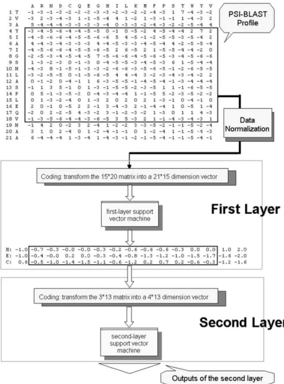
As with Hua and Sun’s work [4], the present analysis used the classical local coding scheme of the protein sequences with a sliding window. PSI-BLAST with n rows and 20 columns can be defined for single sequence with n residues. For the first layer in the prediction system, each residue is coded as a 21-dimensional vector, where the first 20 elements of the vector are the corresponding elements in PSI-BLAST matrix and the last unit was added to represent the N- and C-terminus. For the second layer, the vector corresponding to a residue has 4 elements, where the first 3 elements represent the 3 secondary structures (H, E, C). If the window length is

l, the dimension of the feature vector is 21*l for the first layer and 4*l for the second layer.

A dual-layer SVM structure was used in the prediction system (see Fig. 3.1). The first layer is an SVM classifier that classifies each residue of each sequence into the 3

secondary structure classes (H, E, or C). The one-against-rest strategy was used for the multiclass classification, so there were three outputs for each residue. The outputs represent the probability that the residue belongs to that class. Since the consecutive patterns are correlated (e.g., a helix contains at least 4 consecutive patterns, and a sheet contains at least 3 consecutive patterns), the second-layer SVM classifier filtered successive outputs from the first layer. The target outputs of the second layer were the same as the first layer. As with the first-layer SVM, the second layer also uses the one-against-rest strategy, with each residue classified into the class with the largest output value.

This analysis used the radial basis function (RBF) kernel in both the first- and the second-layer SVM, where γ is a parameter to be determined. The analysis used the soft-margin SVM, so the regularization parameter C also needed to be regulated.

1

γ and C₁ were defined as the gamma parameter and the regularization parameter in the first-layer SVM, while γ and ₂ C₂ were defined as the gamma parameter and the regularization parameter in the second-layer SVM. For the CB513 data set,

1

3.3 Quick Radial Basis Function

Protein secondary structure prediction has been tackled by numerous learning algorithms including neural networks, SVM and other famous classifiers, and therefore presents as a classic problem for testing the effectiveness of new techniques. The QuickRBF package, proposed by Ou et al. [5], can be used to conduct the experiments on the most famous data set used in protein secondary structure prediction, RS126. The RS126 data has been well studied in many publications. Also, the same 7-fold partition used by Riis and Krogh [13] is adopted.

According to the experiments done by Ou et al. [5], which conducted both the LIBSVM, proposed by Lin et al. [6], and QuickRBF approaches in the same environment and the same data sets. The detailed accuracy results [5] can be seen in Table 3.1. As the Table shows, the QuickRBF method basically delivers the same level of accuracy with LIBSVM.

Table 3.1: Comparison of classification accuracy of the RS126 data set with PSI-BLAST PSSM profiles

RS126 LIBSVM QuickRBF QuickRBF QuickRBF QuickRBF

Centers All 12000 5000 1000 Set A 74.06 74.14 74.01 73.73 72.71 Set B 77.44 77.01 76.32 75.54 74.76 Set C 74.99 75.01 75.07 74.93 73.85 Set D 73.11 73.69 73.72 72.44 71.44 Set E 74.08 74.19 74.26 73.97 73.14 Set F 76.93 77.23 77.39 77.28 76.12 Set G 73.82 74.27 74.30 74.07 74.36 Average 74.92 75.08 75.01 74.57 73.77

3.4 A Cascade of Fuzzy ARTMAP and QuickRBF Approach

An important performance measure of a machine learning algorithm is its generalization capability. Generalization is characterized by the number of unseen examples correctly predicted by a learning algorithm given sample training data from which to learn. One way of increasing a learning algorithm’s generalization ability is to reduce its error on training data while providing it training data highly representative of the unknown target function. Fuzzy ARTMAP is designed to realize a new minimax learning rule that conjointly minimizes predictive error and maximized generalization, meaning that the system can learn to create the minimal number recognition categories or “hidden nodes” needed to meet the accuracy criterion (least prediction error).

During the training of radial basis function, the mean values for the K basis functions are first randomly selected and replaced by a new grouped mean after distance calculation and category assignation. In this thesis, we take the advantage of the fuzzy ARTMAP which is capable of learning the “hidden units” automatically. Specifically, we have chosen the geometry means of categories resulting from the fuzzy ARTMAP as the center locations instead of the randomly selected and fixed entities chosen from the training set. Therefore, a cascade of fuzzy ARTMAP and QuickRBF approach is proposed and described in this section.

Figure 3.2 shows the geometry mean of a representative category according to Eq. (3.1) when M = 2 in this case.

(

)

(

(

1-

)

,

(

1-

)

, ,

(

1-

)

)

2 1 , , , _{2 1 M1, 2 M 2, 2M,} 1j C j CMj Wj W j W j W j WMj W j C _K = + ₊ + _{+ K} + (3.1)

Referring to Fig. 3.3, the inputs a of ART are representative vectors of _a 21*w dimension. The ART complement-coding preprocessor transforms the _a

21*w-dimensional vector a into the 2*21*w-dimensional vector _A=(_a,ac) _{at the}

a

ART layer a 0

F . A is the input vector to the ART layer_a a 1

F . Similarly, the input to b

1

F is the 2*3-dimensional vector _B=(_b,bc) _{where b represents for classes C, E,}

H encoded as (1 0 0), (0 1 0) and (0 0 1), respectively. The ART vigilance _a parameter ρ_a can be adjusted so that the resulting categories are accordingly changed. Similarly, other parameters such as ρ_b, ρ_ab and β can also alter the learning of the neural network.

A geometry mean procedure is then used to calculate the geometry means of each category. In this thesis, this geometry means are applied to stand for the centers of each category. Replacing the randomly selected centers by the geometry means produced from the fuzzy ARTMAP, the cascade architecture of fuzzy ARTMAP and QuickRBF is achieved as shown in Fig. 3.3.

Fig. 3.2. Geometry mean of hyperbox R_j j W4 j W1 W3j j W2 × j

C

₂ j

C

₁ j

R

3.5 A Dual-Layer QuickRBF Approach

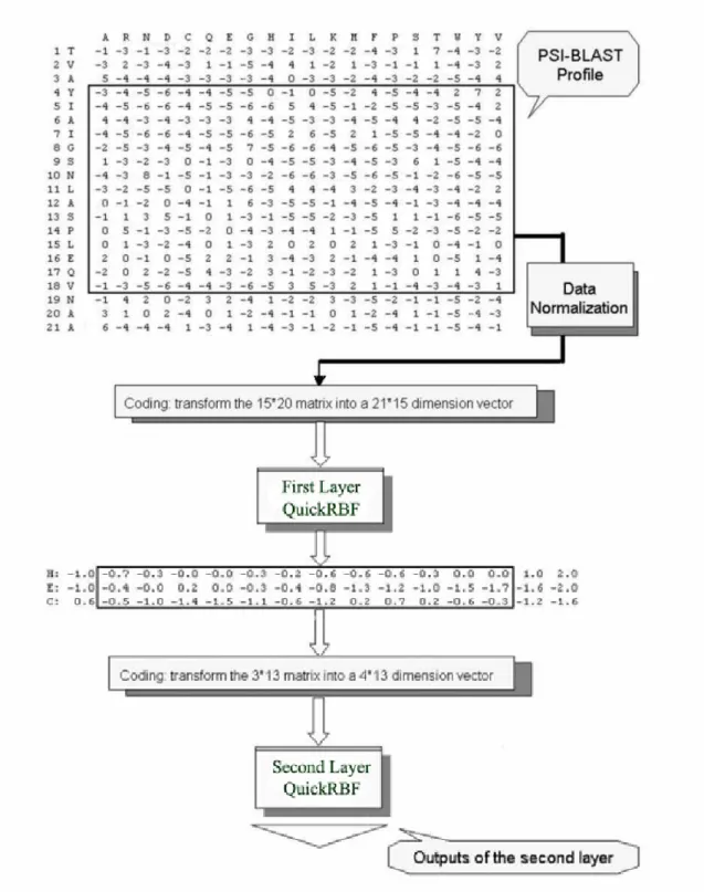
The efficient method was developed for protein secondary structure prediction based on the QuickRBF approaches. QuickRBF is an innovative neural network technology that is capable of delivering the same level of prediction accuracy as the SVM, while enjoying execution efficiency during the phase to construct the classifier.

In this thesis, a dual-layer QuickRBF is conducted as shown in Fig. 3.4. The first layer is a QuickRBF classifier which maps the 21*w dimension representative vector into the 3 classes of PSS (H, E or C). Instead of outputting the class labels, the values of individual output nodes which can be regarded as the probability that the residue belongs to that class for each residue are fed into the second layer after treating the same coding scheme as Hua and Sun [4]. Specifically, the second layer QuickRBF classifies the 4*l vectors and the target outputs of the second layer were the same as the first layer. Finally, each residue is classified into the class with the largest output value.

3.6 Fusion Method

3.6.1 Reliability Index

The prediction reliability index (RI) was used to access the effectiveness of the approaches for the prediction of the secondary structure of a new sequence. The RI offers an excellent tool for focusing on key regions having high prediction accuracy. There are different definitions of the RI. Here we used a definition similar to that proposed by Rost and Sander: RI = maximal_output(I)－Second_largest_output(I). If the value of RI > 0.9, then set RI = 0.9, so the value of RI is between 0 and 0.9. The distribution of the prediction accuracy with different RIs is illustrated in Fig. 3.5. The prediction accuracy of residues with higher RI values is much better than those with lower RI values. Therefore, the definition of RI reflects the prediction reliability.

In this research, to combine the output from the first and second layer, we developed a new classifier design using RI. In this scheme, the output with the maximum RI is chosen as the representative classifier for the final decision of the class. Based on the largest output value of this representative classifier, the final class is chosen. For example, if the output values of the decision function of each classifiers (first layer: C/E/H, second layer: C/E/H) are 0.1/0.2/0.7 and 0.3/0.2/0.5, their RI s are 0.5 (0.7－0.2) and 0.2 (0.5－0.3) respectively. Therefore, the output with highest RI, here the first layer, can be chosen for deciding the final class. Once this representative classifier is selected, the final class is assigned based on the output value of this classifier. In this example, since the largest value of the first layer is the third node, the final class if assigned as helix.

Reliability index distribution of the first and second layer 40 50 60 70 80 90 100 0 0.1 0.2 0.3 0.4 0.5 0.6 0.7 0.8 0.9 Reliability index accu racy in % First Layer Second Layer

Fig. 3.5. The accuracy distribution on different Reliability indices (from 0 to 0.9).

Reliability index distribution of the first and second layer

0 500 1000 1500 2000 2500 3000 3500 4000 4500 0 0.1 0.2 0.3 0.4 0.5 0.6 0.7 0.8 0.9 Reliability index N um be r o f Am in o Ac id First Layer Second Layer

3.6.2 Linear Combination and Weighted Sum Fusion

Since we have proposed the dual-layer QuickRBF approach based on the PSSM profiles to predict the protein secondary structure, we found the difference of predictive results between the first and second layer are somewhat distinct. This motivates us to design a fusion scheme combining the results of each layer in order to raise the overall accuracy. The idea that we have hit upon is the linear combination scheme. Referring to Table 3.2, each residue of the present sequence has three target labels denoted as C, E and H. The respective results of each label are the linear combination of results of the first layer and second layer. Then the final output class of each residue is assigned to the one with the largest output value. Namely, it applies

) ,..., 1 }, , , { ( ) ( max arg ) ( 1 x f x lc C E H j m P _lc lc j = ∈ = (3.1)

where f_lc are the linearly combined values shown as follows:

j j j f j j j f j j j f H H H f E E E f C C C f 2 1 H 2 1 E 2 1 C + = = + = = + = = (3.2)

The next fusion method involves the weighted sum scheme. Referring to Table 3.3, the respective results of three target labels are taken from the weighted sum of the first layer and second layer. The final output class of each residue is assigned to the one with the largest output value. Namely, it applies

) ,..., 1 }, , , { ( ) ( max arg ) ( 2 x f x ws C E H j m P _ws ws j = ∈ = (3.3)

j j j f j j j f j j j f H w H w H f E w E w E f C w C w C f 2 2 1 1 H 2 2 1 1 E 2 2 1 1 C + = = + = = + = = (3.4)

Table 3.2. Fusion method 1: Linear combination.

First-Layer QuickRBF Second-Layer QuickRBF _{(Linear Combination)} Fusion Method 2 Pred 2

Coil Sheet Helix Coil Sheet Helix Coil Sheet Helix Class 1 C11 E11 H11 C21 E21 H21 Cf1 Ef1 Hf1 P11

2 C12 E12 H12 C22 E22 H22 Cf2 Ef2 Hf2 P12

3 C13 E13 H13 C23 E23 H23 Cf3 Ef3 Hf3 P13

… … … … … … … … … … …

m C1m E1m H1m C2m E2m H2m Cfm Efm Hfm P1m

Table 3.3. Fusion method 2: Weighted Sum.

First-Layer QuickRBF Second-Layer QuickRBF Fusion Method 3 _{(Weighted Sum)} Pred 3

Coil Sheet Helix Coil Sheet Helix Coil Sheet Helix Class 1 C11 E11 H11 C21 E21 H21 Cf1 Ef1 Hf1 P21

2 C12 E12 H12 C22 E22 H22 Cf2 Ef2 H f2 P22

3 C13 E13 H13 C23 E23 H23 Cf3 Ef3 Hf3 P23

… … … … … … … … … … …

Chapter 4. Experiment and Results

4.1 Datasets

The set 126 nonhomologous globular protein chains used in the experiment of

Rost and Sander [1], referred to as the RS126 set, was used to evaluate the accuracy of the classifiers. The dataset contained 23606 residues with 32% α-helix, 23% β-strand, and 45% coil. Many current secondary structure prediction methods have been developed and tested on this dataset. The single stage approaches and second-stage approaches were implemented, with multiple sequence alignments, and tested on the dataset, using a sevenfold cross validation technique to estimate the prediction accuracy. With sevenfold cross validation approximately six-seventh of the database was selected for training and, after training, the left one-seventh of the dataset was used for testing. In order to avoid the selection of extremely biased partitions, the RS126 set was divided into seven subsets with each subset having similar size and content of each type of secondary structure as shown in Table 4.1. Referring to Table 4.1, four membrane proteins in the set G are eliminated in this thesis.

Table 4.1. The database of non-homologous proteins used for seven-fold cross validation. All proteins have less than 25% pairwise similarity for lengths great than 80 residues.

4.2 Results

4.2.1 Results of the Cascade of Fuzzy ARTMAP and QuickRBF

For the architecture of the cascade of fuzzy ARTMAP and QuickRBF, we choose a window size of 15 amino acid residues as input according to other benchmark researches such as PSIPRED [14] and SVM [4]. The empirical numbers of categories are about 12000, 10000 and 5000 while the defaulting ρ_a = 0.8, 0.7 and 0.4, respectively. We choose ρ_b = 1 since the encoded classes are linearly independent and orthogonal. We let the map field vigilance parameter ρ_ab be larger

than 0 which means that only the representative vectors holding the same classes will have the chance being learned. The β = 1 which means fast learning is adopted in this thesis.

Table 4.2 shows the performance of the secondary structure predictors using single QuickRBF and cascade of fuzzy ARTMAP (FARTMAP) and QuickRBF on the RS126 set with multiple sequence alignments. The multi-class techniques of the single QuickRBF gave the result for PSS prediction which achieved 75.75% of Q ₃ accuracy while the cascade of the fuzzy ARTMAP and QuickRBF only achieved 73.91%, or even lower.

Table 4.2. Single QuickRBF and cascade of FARTMAP and QuickRBF. RS126 QuickRBF FARTMAP & Cascade of

QuickRBF Cascade of FARTMAP & QuickRBF Cascade of FARTMAP & QuickRBF Centers 5000 12000(ρa=0.8) 10000(ρa=0.7) 5000(ρa=0.4) Set A 75.97 72.25 70.57 68.84 Set B 78.34 76.21 74.89 73.77 Set C 77.01 75.84 73.17 72.15 Set D 72.51 71.35 68.55 67.57 Set E 77.83 75.40 74.24 73.58 Set F 73.26 72.18 69.81 68.22 Set G 76.31 74.44 72.32 71.66 Average 75.75 73.91 71.92 70.77

4.2.2 Results of the Dual-Layer QuickRBF and Fusion Methods

For QuickRBF classifiers at the first stage, similarly we choose a window size of 15 amino acid residues as input. At the second stage, the window size of width 13 is

used as the coding scheme for second-layer QuickRBF technique. The numbers of center selected here were 5000 and 10000 on RS126 which we found the more the numbers of center the better the average accuracy. The first fusion method, linear combination of first and second layers, is determined empirically for optimal performance though the results are only slightly different from the second one. We have used several measures to evaluate the prediction accuracy. The Q3 accuracy indicates the percentage of correctly predicted residues of three states of secondary structure. The Q , _C Q_E , Q_H accuracies represent the percentage of correctly predicted residues of each type of secondary structure.

Tables 4.3 and 4.4 show the performance of the different secondary structure predictors using dual-layer QuickRBF on the RS126 set with multiple sequence alignments. Referring to Table 4.3, the multi-class techniques of first fusion method has an improved accuracy comparing to the results of each layer. It gave the result for PSS prediction which achieved 76.32% of Q accuracy while the accuracy of the ₃ second fusion method was 76.31%. The best result was found to be the first fusion method using reliability index which achieved 76.71% of Q accuracy while the ₃ prediction accuracy obtained by various methods are shown in Table 4.5 for comparison.

Table 4.3. Results of different fusion method with 5000 centers at first stage. RS126 First layer QuickRBF Second layer QuickRBF Fusion Method 1 (RI) Fusion Method 2 (Linear Combine) Fusion Method 3 (Weighted sum) Centers 5000 1000 Set A 74.97 74.62 75.26 75.21 75.23 Set B 78.34 78.28 78.31 78.58 78.55 Set C 77.01 76.77 76.34 77.04 77.08 Set D 72.51 71.92 77.14 72.42 72.39 Set E 77.83 78.54 77.84 79.02 79.01 Set F 73.26 73.31 75.81 75.10 75.05 Set G 76.31 77.16 75.80 77.48 77.40 Average 75.75 75.80 76.42 76.32 76.31

Table 4.4. Results of different fusion method with 10000 centers at first stage. RS126 First layer QuickRBF Second layer QuickRBF Fusion Method 1 (RI) Fusion Method 2 (Linear Combine) Fusion Method 3 (Weighted sum) Centers 10000 1000 Set A 75.62 73.91 74.99 75.14 75.16 Set B 78.37 78.46 79.19 79.16 79.10 Set C 77.31 76.98 76.57 78.09 78.07 Set D 72.42 73.44 77.67 73.49 73.45 Set E 77.97 78.25 78.51 78.35 78.41 Set F 74.27 74.35 76.06 75.98 75.94 Set G 76.20 76.43 75.86 76.75 76.72 Average 76.02 75.97 76.71 76.61 76.60

Referring to Table 4.5, PHD [2]: results obtained from Rost and Sander. DSC, PREDATOR, NNSSP, CONSENSUS [7]: results obtained on the RS126 set from Cuff and Barton. PMSVM [12]: results obtained on CB513 data set from Guo et al.. SVMpsi [23]: results obtaind on RS126 data set from Kim and Park. QRBF [5]: results obtained from the QuickRBF proposed by Ou et al.. dQRBF: results obtained from dual-layer QuickRBF. dfQRBF: results obtained from the first fusion method combining QRBF and dQRBF.

Table 4.5. Results comparison of several methods obtained on RS126 dataset. Method Q (%) 3 Q (%) C QE(%) QH(%) PHD [2] 70.8 72.0 66.0 72.0 DSC [7] 71.1 — — — PREDATOR [7] 70.3 — — — NNSSP [7] 72.7 — — — CONCENSUS [7] 74.8 — — — PMSVM [12] 75.2 72.8 71.5 80.4 SVMpsi [23] 76.1 77.2 63.9 81.5 QRBF [5] 76.0 75.0 63.1 82.9 dQRBF 76.0 77.3 64.3 80.9 dfQRBF 76.7 76.8 64.5 84.7