Multiresolution spectrotemporal analysis of complex sounds
Taishih Chi,a兲Powen Ru,b兲 and Shihab A. Shammac兲
Center for Auditory and Acoustics Research, Institute for Systems Research Electrical and Computer Engineering Department, University of Maryland, College Park, Maryland 20742
共Received 22 June 2004; revised 2 May 2005; accepted 12 May 2005兲
A computational model of auditory analysis is described that is inspired by psychoacoustical and neurophysiological findings in early and central stages of the auditory system. The model provides a unified multiresolution representation of the spectral and temporal features likely critical in the perception of sound. Simplified, more specifically tailored versions of this model have already been validated by successful application in the assessment of speech intelligibility关Elhilali et al., Speech Commun. 41共2-3兲, 331–348 共2003兲; Chi et al., J. Acoust. Soc. Am. 106, 2719–2732 共1999兲兴 and in explaining the perception of monaural phase sensitivity关R. Carlyon and S. Shamma, J. Acoust. Soc. Am. 114, 333–348 共2003兲兴. Here we provide a more complete mathematical formulation of the model, illustrating how complex signals are transformed through various stages of the model, and relating it to comparable existing models of auditory processing. Furthermore, we outline several reconstruction algorithms to resynthesize the sound from the model output so as to evaluate the fidelity of the representation and contribution of different features and cues to the sound percept. ©
2005 Acoustical Society of America. 关DOI: 10.1121/1.1945807兴
PACS number共s兲: 43.66.Ba, 43.71.An, 43.71.Gv 关KWG兴 Pages: 887–906
I. INTRODUCTION
Cochlear frequency analysis has for decades influenced the development of algorithms and perceptual measures for the analysis and recognition of speech and audio. Examples include the formulation of the articulation index 共Kryter, 1962兲 to estimate the effect of noise on speech intelligibility, and the exploitation of models of psychoacoustical masking for the efficient coding of speech and music 共Pan, 1995兲. However, cochlear analysis of sound and the extraction of the acoustic spectrum in the cochlear nucleus are only the earliest stages in a sequence of substantial transformations of the neural representation of sound as it journeys up to the auditory cortex via the midbrain and thalamus. And, while much is known about the neural correlates of sound pitch, location, loudness, and the representation of the spectral pro-file in these early stages, the response properties and func-tional organization in the more central structures of the infe-rior colliculus, medial geniculate body, and the cortex have only begun to be uncovered relatively recently 共deRibaupi-erre and Rouiller, 1981; Kowalski et al., 1996; Schreiner and Urbas, 1988b; Miller et al., 2002; Lu et al., 2001; Egger-mont, 2002; Ulanovsky et al. 2003兲. Consequently, it is less common that one finds ideas from central auditory process-ing beprocess-ing applied in psychoacoustics共Houtgast, 1989; Dau et
al., 1997a, b; Ewert and Dau, 2000; Grimault et al., 2002兲
and in design of speech and audio processing systems共Arai
et al., 1996; Pitton et al., 1996; Greenberg and Kingsbury,
1997; Tchorz and Kollmeier, 1999; Hansen and Kollmeier, 1999; Kleinschmidt et al., 2001; Atlas and Shamma, 2003兲. Interestingly, the opposite has occurred, that is, numerous
useful algorithms and representations that were developed decades ago, based only on engineering intuition, have turned out to be in hindsight grounded on solid auditory neural processing strategies共Hermansky and Morgan, 1994; Atal, 1974兲.
To exploit the accumulating physiological findings from the central auditory system and from psychoacoustic experi-ments, it is essential that they be reformulated as mathemati-cal models and signal processing algorithms. To achieve this objective, this paper provides two specific contributions: 共1兲 It describes a detailed computational model of central
auditory processing. Simplified, specifically tailored, versions of this model have already appeared in previous publications from our group where we demonstrated its successful applications in the objective evaluation of speech intelligibility 共Elhilali et al., 2003; Chi et al., 1999兲 and the perception of phase of complex sounds 共Carlyon and Shamma, 2003兲. Here we provide a more complete mathematical formulation of the model, illus-trating how complex signals are transformed through various stages of the model, and relating it to compa-rable existing models of auditory processing. This ex-panded version of the model is completely consistent with the earlier versions and has been validated to ac-count for the types of signals and distortions considered in earlier publications.
共2兲 It outlines algorithms for reconstructing the input acous-tic signal from its final model outputs. These algorithms are important in that they demonstrate the sufficiency of this model representation by reconstructing faithful rep-lica of the original inputs. They also enable the model to be used in assessing the perceptual significance of vari-ous output features, as well as in applications where a modified final acoustic waveform is necessary such as noise suppression for general audio and hearing aids. a兲Present address: Department of Communication Engineering, National
Chiao Tung University, Hsinchu, Taiwan, Republic of China
b兲Present address: Cybernetics InfoTech Inc. c兲Electronic mail: [email protected]
The model we describe is not biophysical in spirit, but rather it abstracts from the physiological data an interpreta-tion that we believe is likely to be relevant in the design of sound engineering systems. Two particularly important physiological observations are incorporated. The first is the apparent progressive loss of temporal dynamics from the pe-riphery to the cortex. Thus, on the auditory nerve, rapid phase locking to individual spectral components of the stimulus survives up to 4 – 9 kHz. It diminishes to moderate rates of synchrony in the midbrain共under 1 kHz兲, and to the much lower rates of modulations in the cortex 共less than 30 Hz兲1共Kowalski et al., 1996; Miller et al., 2002; Schreiner and Urbas, 1988a; Langner, 1992兲. Another important change in the nature of the neural responses is the emergence of elaborate selectivity to combined spectral and temporal features, selectivity that is typically much more complex than the relatively simple tuning curves and dynamics of auditory-nerve fiber responses 共Nelken and Versnel, 2000; Shamma et al., 1993; Edamatsu et al., 1989兲.
The computational model consists of two major auditory transformations. An early stage captures monaural process-ing from the cochlea to the midbrain. It transforms the acous-tic stimulus to an auditory time-frequency spectrogramlike representation that combines relatively simple bandpass spectral selectivity with moderate temporal dynamics 共⬍1000 Hz兲. The second is called the cortical stage because it reflects the more complex spectrotemporal analysis pre-sumed to take place in mammalian AI. In the following sec-tion, we review the cortical physiological data and psychoa-coustical results that motivated and justified this model’s development. The mathematical formulation of the early and
cortical stages are summarized in Secs. III and IV, together with an illustration of the way in which a variety of complex sounds are represented at each stage. In Sec. V, algorithms to
reconstruct audible approximate versions of the original
sounds from the model’s representations are described. We also provide an example of how the reconstructed signals can be used to assess the contribution of different ranges of spectro-temporal modulations to the intelligibility of speech. Finally, we end in Sec. VI with a summary and a brief as-sessment of the utility of the model in a variety of potential applications.
II. AUDITORY CORTICAL PHYSIOLOGY
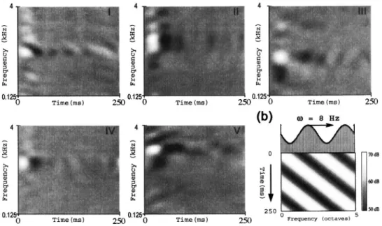
The cortical stage of the model is strongly inspired by extensive data and ideas gained from physiological and psy-choacoustical experiments over the last decade. Specifically, much insight has been gained from measurements of the so-called spectro-temporal response fields 共STRF兲 of AI cells. Examples of a variety of measured STRFs are shown in Fig. 1共a兲. A STRF summarizes the way a cell responds to the stimulus. Along its ordinate—“frequency axis”—the color white depicts acoustic frequencies that excite responses, black denotes frequencies that suppress 共or inhibit兲 sponses, while gray denotes frequency regions of no re-sponse. Thus, some STRFs are responsive 共excited or sup-pressed兲 over a broad range of frequencies, exceeding an octave共ii兲, while others are quite narrowly tuned 共iv兲. Along its abscissa—“Time axis”—the STRF depicts the response dynamics to an “impulse” of energy delivered at each fre-quency. In most STRFs in Fig. 1, the impulse response
con-FIG. 1. Details of the dynamic ripple stimulus and examples of spectrotemporal response fields共STRFs兲 in primary auditory cortex 共A1兲. 共a兲 Example STRFs recorded from A1 of the ferret. White共black兲 color indicates regions of strongly excitatory 共suppressed兲 responses. The STRFs display a wide range of properties from temporally fast共iv兲 to slow 共iii, v兲, spectrally sharp 共iv兲 to broad 共i, ii兲, with symmetric 共iv兲 or asymmetric 共iii兲 inhibition. 共b兲 The moving ripple spectral profile关S共t,x兲兴 is defined by the expression: S共t,x兲=1+A·sin共2·共· t +⍀·x兲+⌽兲, where A is the modulation depth, ⌽ is the phase of the profile,is called ripple velocity共in Hz兲, and ⍀ controls the spectral variation 共or modulation兲—also called ripple density 共in cycles/octave兲. It usually consists of many simultaneously presented tones, depicted schematically by the vertical lines along the frequency axis. The tones are usually equally spaced along the logarithmic frequency axis and spanning 5 oct共e.g., 0.25–8 kHz or 0.5–16 kHz兲. The sinusoidal spectral profile S共t,x兲 is depicted by the dashed curve. The spectrogram of one ripple profile is shown in the bottom panel共⍀=0.4 cycles/octave,= 8 Hz兲.
sists of a damped wave of alternating excitatory共white兲 and inhibitory 共black兲 responses. The response fades rapidly in some STRFs共iv兲, while it lasts twice as long in others 共v兲. Finally, this combined time-frequency sensitivity can take more complex forms that are “inseparable” as in the oriented STRFs of i and iii.
Another way to understand the STRF of a cell is through the implied response selectivity to special test stimuli. STRFs have been measured in many ways 共Calhoun and Schreiner, 1995; deCharms et al., 1998兲, one of which is the “ripple analysis method”共Shamma et al., 1995; Kowalski et
al., 1996; Klein et al., 2000兲. Ripples are broadband noise
with sinusoidally modulated spectrotemporal envelopes with different parameters 关Fig. 1共b兲兴. They serve the same func-tion as regular sinusoids in measuring the transfer funcfunc-tion of linear filters, except that they are two dimensional 共spectral and temporal兲. AI cells respond well to ripples and are usu-ally selective to a narrow range of ripple parameters that reflect details of their spectrotemporal transfer functions. By compiling a complete description of the responses of a cell to all ripple densities and velocities it is possible by an inverse Fourier transform to compute the corresponding STRF.
Therefore, a cell’s STRF and its ripple spectrotemporal transfer functions are uniquely related through the Fourier transform. For instance, broadly tuned cells are most respon-sive to low ripple densities, whereas the opposite is true for narrowly tuned cells. Similarly, STRFs with relatively slug-gish dynamics respond poorly to fast ripple rates. Finally, oriented STRFs imply strong selectivity to correspondingly oriented ripples共i.e., of an appropriate rate-density combina-tion兲. From a functional perspective, the rich variety of STRFs found in AI implies that each STRF acts as a
modu-lation selective filter of its input spectrogram, specifically
tuned to a particular range of spectral resolutions共also called
scales兲 and a limited range of temporal modulations 共or rates兲. The collection of all such STRFs then would
consti-tute a filterbank spanning the broad range of psychoacousti-cally observed scale and rate sensitivity in humans and ani-mals 共Viemeister, 1979; Green, 1986; Dau et al., 1997a; Amagai et al., 1999; Chi et al., 1999兲.
Evidence of the importance of spectrotemporal modula-tions in the perception of complex sounds has come from experiments in which systematic degradations of the speech signal were correlated with the gradual loss of intelligibility 共Drullman et al., 1994; Shannon et al., 1995兲. All such ex-periments have consistently pointed to the importance of the slow temporal 共⬍30 Hz兲 and broad spectral modulations in conveying a robust level of intelligibility 共Drullman, 1995; Fu and Shannon, 2000兲. In fact, the relationship between the temporal modulations and speech intelligibility has long been codified in the formulation of the widely used speech transmission index 共STI兲 共Houtgast et al., 1980兲. In an ex-tension of such ideas, and inspired by the neurophysiological data briefly reviewed here, we formulated and tested a spectro-temporal modulation index共STMI兲 共Chi et al., 1999; Elhilali et al., 2003兲, which assesses the integrity of both the spectral and temporal modulations in a signal as a measure of intelligibility. The STMI proved reliable in capturing the deleterious effects of noise and reverberations, as well as of
previously difficult to characterize distortions such as nonlin-ear compression, phase jitter, and phase shifts共Elhilali et al., 2003兲.
In summary, there is physiological and psychoacoustical evidence that the auditory system, particularly at the level of AI, analyzes the dynamic acoustic spectrum of the stimulus extracted at its earlier stages. It does so by explicitly repre-senting its spectrotemporal modulations by employing arrays of spectrally and temporally selective STRFs. In the remain-der of this paper, we elaborate on the mathematical formula-tion of these computaformula-tions, and detail a method to invert the representations back to the acoustic stimulus so as to hear the effects of arbitrary manipulations.
III. THE EARLY STAGE: THE AUDITORY SPECTROGRAM
Sound signals undergo a series of transformations in the early auditory system and are converted from a one-dimensional pressure time waveform to a two-one-dimensional pattern of neural activity distributed along the tonotopic 共roughly a logarithmic frequency兲 axis. This two-dimensional pattern, which we shall call the auditory
spec-trogram, represents an enhanced and noise-robust estimate of
the Fourier-based spectrogram 共Wang and Shamma, 1994兲. Details of the biophysical basis and anatomical structures involved are available 共Shamma, 1985b; Shamma et al., 1986; Yang et al., 1992兲.
A. Mathematical formulation
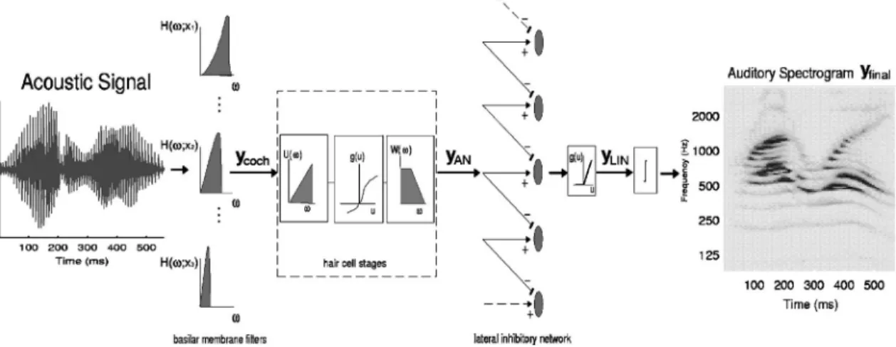
The stages of the early auditory model are illustrated in Fig. 2. In brief, the first operation is an affine wavelet trans-form of the acoustic signal s共t兲. It represents the spectral analysis performed by the cochlear filter bank. This analysis stage is implemented by a bank of 128 overlapping
constant-Q共Q10dB⯝3兲 bandpass filters with center frequencies 共CFs兲
that are uniformly distributed along a logarithmic frequency axis 共x兲, over 5.3 oct 共24 filters/octave兲. The impulse re-sponse of each filter2 is denoted by h共t;x兲. These cochlear filter outputs ycoch共t,x兲 are transduced into auditory-nerve
patterns yAN共t,x兲 by a hair cell stage consisting of a
high-pass filter, a nonlinear compression g共·兲, and a membrane leakage low-pass filter w共t兲 accounting for decrease of phase-locking on the auditory nerve beyond 2 kHz. The final transformation simulates the action of a lateral inhibitory network 共LIN兲 postulated to exist in the cochlear nucleus 共Shamma, 1989兲, which effectively enhances the frequency selectivity of the cochlear filter bank 共Lyon and Shamma, 1996; Shamma, 1985b兲. The LIN is simply approximated by a first-order derivative with respect to the tonotopic axis and followed by a half-wave rectifier to produce yLIN共t,x兲. The
final output of this stage is obtained by integrating yLIN共t,x兲
over a short window, 共t;兲=e−t/u共t兲, with time constant
= 8 ms mimicking the further loss of phase locking observed in the midbrain. The mathematical formulation for this model can be summarized as follows:
ycoch共t,x兲 = s共t兲丢th共t;x兲, 共1兲
yLIN共t,x兲 = max共xyAN共t,x兲,0兲, 共3兲
yfinal共t,x兲 = yLIN共t,x兲丢t共t;兲, 共4兲
where丢tdenotes convolution operation in the time domain.
The model described above attempts to capture many of the important properties of auditory processing that are criti-cal for our objectives and further detailed in the following sections. In creating such a computational model, one has to balance many conflicting requirements and hence make com-promises on what simplifications to apply and what details to include. For instance, our cochlear filtering is essentially lin-ear, lacking such phenomena as two-tone suppression and level-dependent tuning, which are critical in some applica-tions 共Carney, 1993兲. The lateral inhibition model is very schematic and lacks details of single neurons 共Shamma, 1989兲. We also have no explicit adaptive properties in our current model共Westerman and Smith, 1984; Meddis et al., 1990; Dau et al., 1996兲. All of these details are likely to be important in certain circumstances and should be added when needed共Cohen, 1989兲.
B. Examples of the auditory spectrogram
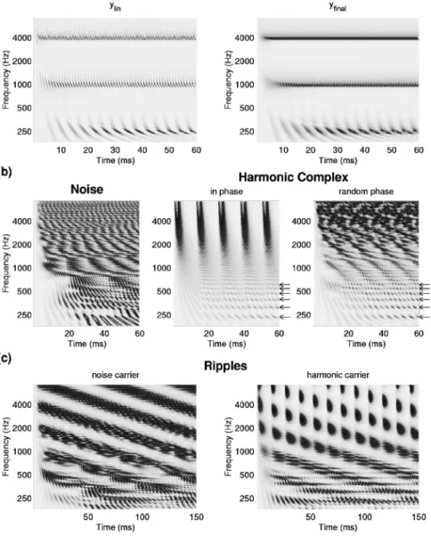
Examples of the information preserved at the LIN output 关yLIN共t,x兲兴 and midbrain levels 关yfinal共t,x兲兴 of the model are
described for five types of progressively more complex stimuli; a three-tone combination, noise, a harmonic com-plex, ripples, and speech and music segments. Understanding details of the auditory spectrogram yfinal共t,x兲 is important
since it serves as the input to the cortical analysis stage as we discuss in the next section.
1. Three tones: 250, 1000, and 4000 Hz
Figure 3共a兲 illustrate the response patterns due to a low-, medium-, and high-frequency tones. The low-frequency tones 共250 and 1000 Hz兲 evoke the typical traveling-wave phase-locked patterns observed experimentally in the audi-tory nerve共Pfeiffer and Kim, 1975; Shamma, 1985a兲. For the high-frequency tone, phase locking is lost and only the en-velope is preserved. These patterns remain the same at the
midbrain stage except that the upper limit of phase locking decreases to below 1000 Hz. Thus, in the right panel of Fig. 3共a兲, substantial phase locking is only seen for the 250-Hz tone.
2. Noise
Figure 3共b兲 共left panel兲 depicts the yfinal共t,x兲 generated
by a broadband noise constructed with 59 random-phase tones that are equally spaced共0.1 oct兲 on a logarithmic fre-quency axis 共135–7465 Hz兲. At this intertone spacing, two to four tones interact within each constant-Q cochlear filter, producing a modulated carrier at the CF of each filter. The envelope modulations at each filter reflect its bandwidth and the intertone spacing in the stimulus. In the low frequency regions共⬍1000 Hz兲, the output 关yfinal共t,x兲兴 captures both the
carrier and envelope. At higher CF regions, the predominant representation is that of the envelopes as carrier phase-locking diminishes. Note that the modulation rates of the envelope increase共in Hz兲 with CF as filter bandwidths and stimulus intertone spacing become wider. Maximum rates are limited by maximum filter bandwidths, and hence do not exceed a few hundred Hertz in most mammals 共Joris and Yin, 1992兲.
3. Harmonic complexes
Unlike broadband noise, harmonic complexes have uni-form intertone spacing equal to the fundamental frequency of the harmonic series. Consequently, the fundamental compo-nent and low-order harmonics remain well resolved by the filters, whereas many high-order harmonics fall within the bandwidth of a cochlear filter at high CFs. Figure 3共b兲 共middle panel兲 illustrates the responses to in-phase harmonic series stimulus with the fundamental at 80 Hz. Low-order harmonics 共⬍8th兲 are well resolved 共as indicated by the ar-rows兲, each dominating the response within one filter, and hence there are little envelope modulations. At high CFs, the unresolved higher harmonics interact, producing the strong 80-Hz periodic envelope modulations. When the harmonics are random phase 关Fig. 3共b兲, right panel兴, the envelope modulations become irregular and less peaked, but still
pre-FIG. 2. Schematic of early auditory stages. The acoustic signal is analyzed by a bank of constant-Q cochlear-like filters. The output of each filter共ycoch兲 is
processed by a hair cell model共yAN兲 followed by a lateral inhibitory network, and is finally rectified 共yLIN兲 and integrated to produce the auditory spectrogram
serve their periodicity of 80 Hz. The key general observation to make about these envelope modulations is that they relate to intercomponent interactions, and hence are affected by the spacing, phase, and relative amplitudes of the components— factors reflecting the perceptual timber of the sound. In the next two example stimuli, we distinguish these intermediate rate modulations from slow modulations created by produc-tion mechanisms which, in speech and music, strongly determine the intelligibility of speech and identity of an instrument.
4. Ripples: Spectrotemporally modulated noise
The model’s outputs for a spectro-temporal modulated broadband noise—also called a ripple—are shown in Fig. 3共c兲 共left panel兲. The stimulus is generated by amplitude modulating each of the 59 components of the noise described earlier in Fig. 3共b兲 共left panel兲 so as to produce a spectrotem-poral profile as depicted in Fig. 1共b兲. Detailed definition and description of these stimuli can be found in Chi et al.共1999兲 and Kowalski et al.共1996兲.
The left panel of Fig. 3共c兲 displays the yfinaloutput for a
downward sweeping ripple 共= 16 Hz,⍀=1 cycle/octave兲.
At low CFs 共Ⰶ1000 Hz兲, the responses exhibit temporal modulations at three different time scales simultaneously. The slow modulations 共16 Hz兲 reflect the spectrotemporal sinusoidal envelope of the ripple. They ride on top of the
intermediate modulations due to component interactions
共30–400 Hz兲. These in turn ride on one top of the fast re-sponses phase locked to the tones of the stimulus. At high CFs, only the slow and intermediate modulations survive. At very low CFs共⬍250 Hz兲, slow and intermediate modulation rates may become comparable due to the narrower band-widths of the filters, and hence the distinct view of the ripple modulations deteriorates.
Figure 3共c兲 共right panel兲 illustrates the responses to the
same ripple spectrotemporal envelope, but this time carried
by the harmonic series of Fig. 3共b兲 共middle panel兲. The slow modulations are again well represented in the responses, but this time riding on a totally different pattern of intermediate modulations that reflect the 80-Hz periodicity of the funda-mental. It is in this sense that we distinguish between these two types of envelope modulations: the intermediate are strictly due to component interactions whereas the slow modulations are superimposed on top and are related to the evolution of the spectrum, e.g., from one syllable to another
FIG. 3. Examples of early auditory re-sponses for progressively more complex stimuli. 共a兲 A three-tone 共250,1000,4000 Hz兲 combination; left panel shows the response at the LIN output 关yLIN共t,x兲兴 and right panel shows the
re-sponse at midbrain level of the model 关yfinal共t,x兲兴. 共b兲 The midbrain output
yfinal共t,x兲 to a broadband noise 共left兲,
broad-band in-phase harmonic complex共middle兲, and a broadband random-phase harmonic complex共right兲. 共c兲 The yfinal共t,x兲 output to
a spectro-temporally modulated noise共left兲 and spectro-temporally modulated in-phase harmonic series 共right兲. All stimuli are sampled at 16 kHz.
in speech, or from one note or instrument to another in music 共see next example兲.
5. Speech and music
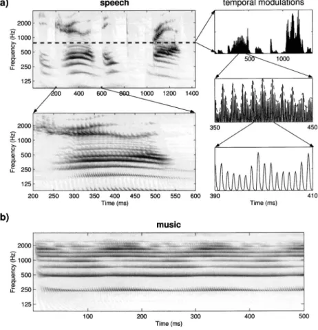
Speech and music are an elaboration of harmonic or noise ripples in that they are conceptually constructed of a spectrotemporal envelope superimposed on a broadband noise or harmonic complex. Figure 4共a兲 shows the yfinal共t,x兲
responses in detail to the utterance /He drew a deep breath/ spoken by a male speaker. Figure 4共b兲 displays the responses to the B3 note played on a bowed violin. Both responses exhibit similar features to those of the ripple. For example, it is possible to see in Fig. 4共a兲 the three kinds of temporal modulations, as highlighted for one channel共at 750 Hz兲 in the three right panels. Here the slow modulations that reflect the syllabic rates of speech 共top panel兲 are superimposed upon the intermediate rate modulations due to unresolved harmonics 共⬇100 Hz兲 of the fundamental pitch 共middle panel兲, which in turn are riding upon the phase-locked re-sponses to the acoustic energy near 750 Hz共bottom panel兲. Also evident in the spectrograms are the spectral modula-tions created by the resolved harmonics共⬍500 Hz兲, and the second and third formants 共⬎750 Hz兲. The same types of modulations are seen in the violin sound in Fig. 4共b兲. Note especially the slow modulations encoding the gradual onset of the note, and the periodic modulations at⬇6 Hz seen in most channels responses. As in speech, these slow features reflect primarily motor production mechanisms due to the fingering共vibrato兲 and bowing characteristics.
The distinction between these three types of temporal scales共fast, intermediate, and slow兲 is essentially identical to one already proposed by Stuart Rosen 共Rosen, 1992兲. In an incisive article, he dissected the acoustic speech waveform into these three time scales and related them to the various auditory and production aspects just as described above. The one point to emphasize here is that the temporal scales de-fined here are made with respect to the channel responses
after the early auditory analysis rather than the original
acoustic waveform关or as Rosen calls it, the normal hearing case共Rosen, 1992兲 兴.
IV. THE CORTICAL STAGE: SPECTROTEMPORAL ANALYSIS
The second analysis stage mimics aspects of the re-sponses of higher central auditory stages共especially the pri-mary auditory cortex兲. Functionally, this stage estimates the spectral and temporal modulation content of the auditory spectrogram. It does so computationally via a bank of filters that are selective to different spectrotemporal modulation pa-rameters that range from slow to fast rates temporally, and from narrow to broad scales spectrally. The spectrotemporal receptive fields共STRFs兲 of these filters are also centered at different frequencies along the tonotopic axis 共Chi et al., 1999兲.
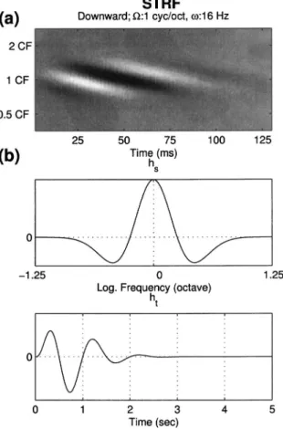
An example of the STRF of such a filter in the bank is shown in Fig. 5共a兲. Three features are of particular interest: 共i兲 it is centered on a particular center frequency 共CF兲. The location of the excitatory 共white兲 and inhibitory 共black兲 stripes on the vertical axis indicates that it is sensitive to
FIG. 4. Examples of auditory spectrograms 关yfinal共t,x兲兴 for speech and music stimuli. 共a兲
The auditory spectrogram of the utterance /He drew a deep breath/ spoken by a male with a pitch of approximately 100 Hz. The dashed line marks the auditory channel at 750 Hz whose temporal modulations are depicted to the right at different time scales. At the coarsest scale共top panel兲, the slow modulations 共few Hz兲 roughly correlate with the different syllabic segments of the utterance. At an intermediate scale共middle panel兲, modulations due to interharmonic inter-actions occur at a rate that reflects the funda-mental共100 Hz兲 of the signal. This is clearly shown by the dashed line envelope of the re-sponse. At the finest scale共bottom panel兲, the fast temporal modulations are due to the fre-quency component driving this channel best 共around 750 Hz兲. 共b兲 The auditory spectrogram of the note共B3兲 played on a violin. Again, note the modulations of the energy in time, especially at the higher CF channels 共⬎1500 Hz兲.
frequencies of about a 2-oct range around the CF共between about 0.5 CF and 2 CF兲; 共ii兲 the modulation rate along the time axis is about 16 Hz; and共iii兲 the excitatory portions are separated on the vertical axis by about 1 oct, giving rise to a spectral “scale” sensitivity to peaks separated by 1 oct, or a scale of 1 cycle/ octave. Finally, the bars sweep downwards diagonally from the top left, which is denoted in the model by assigning a positive sign to the rate parameter; bars sweeping up from bottom left to top right are designated by negative rate values. This distinction reflects the differential sensitivity of neurons in the auditory cortex to the direction in which spectral peaks move共Depireux et al., 2001兲.
The filter output is computed by a convolution of its STRF with the input auditory spectrogram关yfinal共t,x兲兴, i.e., it
is a modified spectrogram. Note that the spectral and tempo-ral cross sections of a filter’s STRF are typical of a bandpass impulse response in having alternating excitatory 共positive兲 and inhibitory共negative兲 fields. Consequently, the filter out-put is large only if the spectrotemporal modulations are com-mensurate with the rate, scale, and direction of the STRF. That is, each filter will respond best to a narrow range of these modulations. The output of the model consists of a map of the responses across the filter bank, with different stimuli being differentiated by which filters they activate best. The response map provides a unique characterization of the spec-trogram, one that is sensitive to the spectral shape and
dy-namics of the entire stimulus. We now provide a mathemati-cal formulation of the STRFs and procedures to compute, display, and interpret the model outputs.
A. Mathematical formulation
We assume a bank of “idealized” STRFs as depicted in Fig. 5共a兲. Each STRF is selective to a narrow range of tem-poral and spectral modulations and is also directionally sen-sitive to either upward or downward drifting modulations. A complete set of such STRFs with a range of temporal and spectral selectivity 共e.g., 1–300 Hz, and 0.25–8 peaks or cycles/octave兲 would be sufficient to decompose and charac-terize the modulations in the auditory spectrogram. More re-alistic complex STRFs can be readily formed by superposi-tion of these basic STRFs.
We define the STRF as a real function that is formed by combining two complex functions in a manner consistent with extensive physiological data. Specifically, experimental STRFs are not necessarily time-frequency separable. Instead, we have found that they are almost always so-called “quad-rant separable.”3This requires that the STRF be represented as the real of the product of a complex temporal and a com-plex spectral “impulse response” function, hIRT共t兲 and
hIRS共x兲, as follows: STRF⬅R兵hIRT共t兲·hIRS共x兲其, where
hIRS共x;⍀,兲 = hirs共x;⍀,兲 + jhˆirs共x;⍀,兲, 共5兲
hIRT共t;,兲 = hirt共t;,兲 + jhˆirt共t;,兲. 共6兲
R兵·其 denotes the real part, and h共·兲 and hˆ共·兲 denote Hilbert
transform pairs. The real functions hirs共·兲 and hirt共·兲 are
de-fined by sinusoidally interpolating seed functions hs共·兲, ht共·兲
and their Hilbert transforms 共Wang and Shamma, 1995兲,
hirs共x;⍀,兲 = hs共x;⍀兲cos+ hˆs共x;⍀兲sin, 共7兲
hirt共t;,兲 = ht共t;兲cos+ hˆt共t;兲sin, 共8兲
where⍀ andare the spectral density and velocity param-eters of the filters; and are characteristic phases; hs共·兲
and ht共·兲 are the spectral and temporal functions that
deter-mine the modulation selectivity of the STRF, and hˆs共·兲 and
hˆt共·兲 are their Hilbert transforms. In addition, the directional
sensitivity of the STRF is modeled as STRF⇓=R兵hIRT共t兲 · hIRS共x兲其,
STRF⇑=R兵hIRT
* 共t兲 · h
IRS共x兲其,
where ⴱ denotes the complex conjugate; ⇓ and ⇑ denote downward and upward moving direction respectively. Note, the downward STRF shown in Fig. 5共a兲 is a special case of == 0.
We choose hs共·兲 to be a Gabor-like function 关commonly
used in the vision literature to describe the analogous spatial aspect of a receptive field 共Jones and Palmer, 1987兲兴. It is defined as the second derivative of a Gaussian function; ht共·兲
is assumed to be a gamma function 关e.g., as in Slaney 共1998兲兴. Both are depicted in Fig. 5共b兲,
FIG. 5. A representative STRF and the seed functions of the spectrotempo-ral multiresolution cortical processing model.共a兲 An example of a STRF in the model. It is upward selective and tuned to共1 cycle/octave,16 Hz兲. 共b兲 Seed functions共noncausal hsand causal ht兲 used to generate all STRFs of
the model. The abscissa of each figure is normalized to correspond to the tuning scale of 1 cycle/ octave or rate of 1 Hz.
hs共x兲 = 共1 − x2兲e−x
2/2 ,
ht共t兲 = t2e−3.5tsin共2t兲,
and for different scales and rates,
hs共x;⍀兲 = ⍀hs共⍀x兲,
ht共t;兲 =ht共t兲.
Therefore, the STRF in general is an inseparable spec-trotemporal function of hs共·兲 and ht共·兲, with a specific highly
constrained spectrotemporal structure known as “quadrant separable.”
The spectrotemporal response of a downward共upward兲 cell c for an input spectrogram y共t,s兲 is then given by
rc⇓共⇑兲共t,x;c,⍀c,c,c兲
= y共t,x兲丢txR兵关hIRT共ⴱ兲共t;c,c兲 · hIRS共x;⍀c,c兲兴其, 共9兲
where 丢txdenotes convolution with respect to both t and x.
This multiscale multirate 共or multiresolution
spectrotempo-ral兲 response is called “cortical representation.” Substituting
Eqs.共5兲–共8兲 into Eq. 共9兲, the cortical representation at down-ward or updown-ward cell c can be rewritten as
rc⇓共t,x;c,⍀c,c,c兲 = y共t,x兲丢tx关共hths− hˆthˆs兲cos共c+c兲 +共hˆths+ hthˆs兲sin共c+c兲兴 共10兲 and rc⇑共t,x;c,⍀c,c,c兲 = y共t,x兲丢tx关共hths+ hˆthˆs兲cos共c−c兲 +共hˆths− hthˆs兲sin共c−c兲兴, 共11兲
where ht⬅ht共t;c兲 and hs⬅hs共x;⍀c兲 to simplify notation.
A useful reformulation of the response rcis in terms of
the output magnitude and phase of a two-dimensional com-plex wavelet transform as follows. Let
z⇓共t,x;c,⍀c兲 = y共t,x兲丢tx关hTW共t;c兲hSW共x;⍀c兲兴
=兩z⇓共t,x;c,⍀c兲兩ej⇓共t,x;c,⍀c兲, 共12兲
z⇑共t,x;c,⍀c兲 = y共t,x兲丢tx关hTW* 共t;c兲hSW共x;⍀c兲兴
=兩z⇑共t,x;c,⍀c兲兩e
j⇑共t,x;c,⍀c兲, 共13兲
with hSW共·兲 and hTW共·兲 defined as
hSW共x;⍀c兲 = hs共x;⍀c兲 + jhˆs共x;⍀c兲, 共14兲
hTW共t;c兲 = ht共t;c兲 + jhˆt共t;c兲. 共15兲
Substituting Eqs. 共14兲 and 共15兲 into Eqs. 共12兲 and 共13兲 and comparing with Eqs. 共10兲 and 共11兲, the cortical response at cell c can be simplified to
rc⇓共t,x;c,⍀c,c,c兲
=R兵z⇓其cos共c+c兲 + I兵z⇓其sin共c+c兲
=兩z⇓兩cos共⇓−c−c兲 共16兲
and
rc⇑共t,x;c,⍀c,c,c兲
=R兵z⇑其cos共c−c兲 − I兵z⇑其sin共c−c兲
=兩z⇑兩cos共⇑+c−c兲 共17兲
where z⇓⬅z⇓共t,x;c,⍀c兲, z⇑⬅z⇑共t,x;c,⍀c兲, ⇓
⬅⇓共t,x;c,⍀c兲, and ⇑⬅⇑共t,x;c,⍀c兲 for short
nota-tion; R兵·其 and I兵·其 denote the real part and imaginary part, respectively.
The expressions above show that the cortical model re-sponse rc can be reexpressed in terms of magnitude
re-sponses兩z⇓兩,兩z⇑兩 and phase responses ⇓,⇑, which are ob-tained by complex wavelet transform 关Eqs. 共12兲 and 共13兲兴. Clearly, the magnitude responses 兩z⇓共t,x;c,⍀c兲兩 and
兩z⇑共t,x;c,⍀c兲兩 represent the maximal downward 共⇓=c
+c兲 and upward 共⇑= −c+c兲 cortical responses at
loca-tion共t,x;c,⍀c兲.
B. Examples of cortical representations
Because of the multidimensionality of the cortical re-sponse rc, displaying it in an intuitive manner is not trivial,
requiring user judgment as to which dimensional views pro-vide the best insights. We illustrate next a variety of such views for the stimuli discussed earlier in Sec. III.
1. Three tones
Figure 6共a兲 shows three particularly useful summary views of the cortical responses to the three-tone auditory spectrogram in Fig. 3共a兲. These three displays are generated by first integrating兩z⇓兩,兩z⇑兩 over their duration, i.e., removing their dependence on t and becoming three dimensional. Next, to generate each of the 2-D panels in Fig. 6共a兲, the remaining third variable is integrated out over its domain. For example, in the left panel, the dependence on scale共⍀c兲 is removed by
integrating all STRF outputs along this dimension, hence emphasizing the representation of temporal modulations 共rate兲 at each CF. Since this stimulus is stationary 共sustained tones兲, it evokes only very low rate outputs 共c艋4 Hz兲 at
each of the three tone frequencies. There is, however, a strong output at x andcof 250 Hz due to the phase-locked
responses of this tone 关seen in the auditory spectrogram of the stimulus in Fig. 3共a兲兴; a weaker output due to phase lock-ing is also seen at 1 kHz. Note also that both phase-locked responses are much stronger in the “Downward” panel of the display because of the traveling wave delay evident in the spectrograms of Fig. 3共a兲.
The center panel of Fig. 6共a兲 displays the output in the scale-frequency plane, integrating all filter outputs along the rate axis. STRFs with fine resolution relative to the intertone 2-oct spacing 共i.e., tuned to ⍀c⬎0.5 cycle/octave兲 respond
to each tone separately. STRFs with broad bandwidths 共⍀c
into one broad peak. A “bifurcation” point emerges around the scale at which the peaks become resolved共⍀c⬇0.5兲.
The right panel is particularly useful in summarizing the conjunction between the temporal and spectral modulations in a spectrogram. As expected, strong response can be seen at very low rate艋4 Hz and at 0.5 cycle/octave 共since the tones are separated by 2 oct兲. A strong 250-Hz phase-locked re-sponse is also seen here but has been smeared out along the scale axis. Note, the frequency axis is integrated out, and hence the display is insensitive to pure translations of the spectrum along the x axis.
2. Noise and harmonic complexes
Like the tones, both stimuli here are stationary. How-ever, the drastically different nature of their envelope modu-lations and underlying spectra creates distinctive cortical out-puts as shown in Figs. 6共b兲 and 6共c兲.
The noise evokes a rate-frequency response 关Fig. 6共b兲, top panel兴 which captures the increase in intermediate-rate
temporal modulations with increasing CF 共marked by the dashed line兲 due to the increasing bandwidth of the cochlear filters as discussed in Fig. 3共b兲 earlier. By contrast, the re-sponse to the harmonic stimulus 关top panel of Fig. 6共c兲兴 is dominated by the phase-locked responses to the resolved low-order harmonics, and all intermediate-rate modulations at high CF 共艌1000 Hz兲 occur at a rate=80 Hz 共marked by the dashed line兲. Finally, both panels exhibit larger energy in the “downward”-half of the plot due the accumulating phase lag of the cochlear filters 共the well-known “traveling waves”兲.
The scale-frequency panels共bottom panels兲 of Figs. 6共b兲 and 6共c兲 illustrate the contrast between the irregular versus regular nature of the two stimulus spectra. Note especially the distinctive and typical pattern associated with harmonic spectra in which “bifurcation” points shift systematically up-wards, indicating the increasing crowding of the higher har-monics along the x axis.
FIG. 6. Examples of cortical representations for stimuli as in Fig. 3:共a兲 a three-tone 共250,1000,4000 Hz兲 combination, 共b兲 a broadband noise, 共c兲 broadband in-phase harmonic complex, and共d兲 ripples. For each of these stationary stimuli, the four-dimensional representation 兩z⇓兩, 兩z⇑兩 is first integrated over time to generate a three-dimensional representation. For the three-tone combinations, each of the remaining three variables共scale, rate, frequency兲 is integrated out over its domain to display these 2-D representations at left, center, and right panels of共a兲, respectively. For the broadband noise 关in 共b兲兴 and in-phase harmonic complexes关in 共c兲兴, the top and bottom panels demonstrate the rate-frequency and scale-frequency cortical representations. The top and bottom panels of 共d兲 show the scale-rate representations of a downward noise ripple共top兲 and an upward harmonic ripple 共bottom兲, both modulated at 16 Hz, 1 cycle/octave. In each plot, the negative共positive兲 rate denotes upward 共downward兲 moving direction.
3. Ripples
Ripples with a single sinusoidal spectrotemporal modu-lation activate mostly STRFs with the corresponding selec-tivity. This is best illustrated by the localized response pat-tern in the scale-rate views of Fig. 6共d兲 due to a downward noise ripple共top panel兲 and an upward harmonic ripple 共bot-tom panel兲. Regardless of the carrier, both ripples activate a localized response that captures the rate and scale of the slow modulations in the stimulus. Details of other views, however, would distinguish the two ripples from each other.
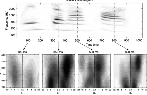
4. Speech and music
Speech and music are typically nonstationary, with spec-trotemporal modulations that change their parameters. Con-sequently, it is often important to view the time evolution of the response patterns. Figure 7 illustrates one possible repre-sentation of the model outputs as a distribution of activity in the scale-rate plane as different phonemes and syllables are analyzed by the model. As before, these panels are computed by first integrating兩z⇓兩,兩z⇑兩 over frequency x, and then plot-ting the scale rate as a function of the third axis t.
These plots can uniquely summarize the salient features of the underlying spectrogram, and hence may potentially serve as efficient descriptors of the underlying speech seg-ments. For instance, the downward-sweeping harmonic peaks near 350 and 800 ms generate strongly asymmetric patterns in the second and forth panels. The opposite sym-metry is seen near 100 ms where the formant is sweeping upwards. Along the spectral dimensions, the main
concentra-tion of energy in the spectrogram shifts upwards from near 500 Hz at 100 ms 共second harmonic兲 to 700 Hz at 350 ms 共third harmonic兲, to near 1000 Hz at 800 ms 共fourth and fifth harmonics兲. Consequently, the concentration of energy along the scale axis共illustrated in the lower series of panels兲 shifts upwards from near 1 cycle/ octave 共at 100 ms兲, to 2 cycles/ octave 共at 350 ms兲, to about 4 cycles/octave 共at 800 ms兲. For further examples of such an analysis, please refer to Shamma共2003兲.
V. RECONSTRUCTION
We derive in this section computational procedures to resynthesize the original input stimulus from the output of early auditory and cortical stages. While the nonlinear opera-tions in the early stage make it impossible to have perfect reconstruction, perceptually acceptable renditions are still feasible as we shall demonstrate. The ability to reconstruct the audio signal from the final representation is extremely useful in building the intuition of the role of different spec-trotemporal cues in shaping the timbre percept as we shall elaborate in this section. Furthermore, it provides indirect measure of the fidelity and completeness of the representa-tion as well as a potential means for manipulating timbre of musical instruments, morphing speech, and changing voice quality.
A. Reconstruction from auditory spectrogram
The most important component of the forward analysis stage—the linear filter bank operation 关Eq. 共1兲兴—is
invert-FIG. 7. The cortical multiresolution spectrotemporal representation of speech. The auditory spectrogram of the speech utterance /We’ve done our part/ spoken by a female speaker. The four bottom panels display scale-rate representation of the model output at the time instants marked by the vertical dashed lines in the auditory spectrogram. Each panel displays the spectrotemporal distribution of responses over the recent past共several 100 ms兲. For instance, the asym-metric responses at 350 ms reflect the downward shift in the pitch or frequency of all harmonics near the onset of the syllable共300 ms兲. They peak near 6 – 10 Hz because of the intersyllable time interval of about 120– 180 ms共between the first and second syllables—/we’ve/ and /done/兲. They also peak at 2 cycle/ octave because most of the spectral energy occurs near the second and third harmonics共which are separated by about 0.5 oct兲.
ible and the inverse operation can be derived as follows 共Akansu and Haddad, 1992兲. From Eq. 共1兲,
Ycoch共,x兲 = S共兲H共;x兲 ⇒
兺
x Ycoch共,x兲H*共;x兲 共18兲 =S共兲兺
x H共;x兲H*共;x兲 ⇒ S共兲 =兺
x Ycoch共,x兲H*共;x兲冒
兺
x 兩H共;x兲兩2, where Ycoch共, x兲, S共兲, and H共; x兲 are the Fouriertrans-forms of ycoch共t,x兲, s共t兲, and h共t;x兲 respectively. The overall
response of the filter bank,兺x兩H共; x兲兩2, is flat except at the
lowest and highest frequency skirts where it drops precipi-tously, causing large noise and numerical errors in the inver-sion procedures. To avoid this problem, we shall simply ig-nore the response at these extreme frequencies and make the overall response unitary within the remaining band by intro-ducing a real-valued weighting function W共x兲:
H1共;x兲 = W共x兲H共;x兲 such that
兺
x
兩H共;x兲兩2W共x兲 ⯝ 1
within the effective band. Therefore, the time waveform s˜共t兲
can be computed from the projected filter bank response
y ˜coch共t,x兲 关Eq. 共18兲兴: S ˜共兲 =
兺
x Y ˜ coch共,x兲H1*共;x兲, 共19兲 s ˜共t兲 =兺
x y ˜coch共t,x兲丢th1 *共− t;x兲 =兺
x y ˜coch共t,x兲丢th1共− t;x兲. The reconstruction from the envelope yfinal共t,x兲 back toycoch共t,x兲 is difficult to derive directly through the two
non-linear functions g共·兲 and max共·,0兲. Instead, an iterative method based on the convex projection algorithm proposed in Yang et al.共1992兲 is used to reconstruct s共t兲. The method is summarized in the following steps:
共1兲 Initialize a Gaussian distributed white noise with zero-mean and unit variance, i.e., s˜共k兲共t兲⬃N共0,1兲, and set the
iteration counter k = 1. 共2兲 Compute y˜coch
共k兲 共t,x兲 and all the way to y˜
final
共k兲 共t,x兲 with respect to s˜共k兲共t兲.
共3兲 Find the ratio r共k兲共t,x兲 between the target y
final共t,x兲 and
y
˜共k兲final共t,x兲.
共4兲 Scale the filter-bank response, i.e., y˜coch
共k兲 共t,x兲←r共k兲共t,x兲 ⫻y˜coch
共k兲 共t,x兲.
共5兲 Reconstruct time waveform s˜共k+1兲共t兲 by inverse filtering 关Eq. 共19兲兴, and update counter k=k+1.
共6兲 Go to step 2 unless certain criteria are met 关e.g., the distortion rate of y˜final共k兲 共t,x兲 or the number of iteration兴.
Note, the auditory spectrogram yfinal共t,x兲 is assumed roughly
representing a local time-frequency共TF兲 energy distribution, and hence the estimated y˜coch共t,x兲 can be adjusted by the
ratio of the target yfinal共t,x兲 divided by the computed
spec-trogram y˜final共t,x兲 pertaining to y˜coch共t,x兲. Figure 8 illustrates
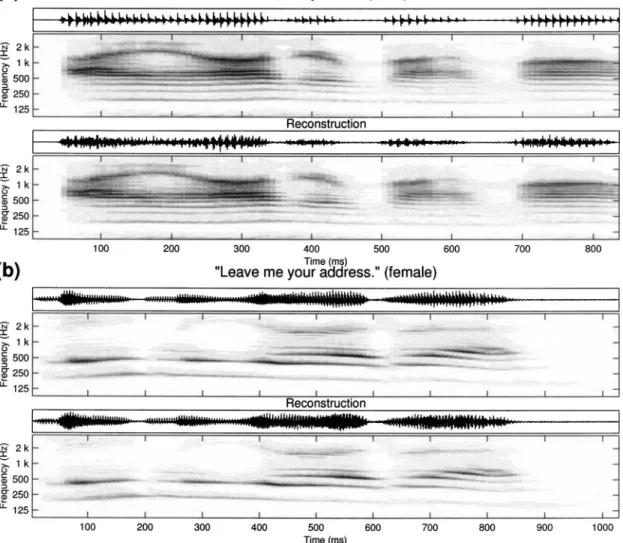
the similarity between original and reconstructed auditory spectrograms of two speech utterances after 100 iterations. Note that although this iterative algorithm does not give a unique reconstructed waveform because of the loss of the phase of the original components, the quality of recon-structed sounds using different initial conditions is very close and is reasonably similar to the original signal as can be heard at http://www.isr.umd.edu/CAAR/pubs.html. We shall discuss later in this section an objective assessment of the quality of this reconstructed speech using the mean opinion score共MOS兲 as quantified by the “perceptual evaluation of speech quality” 共PESQ兲 index available from http:// www.itu.int/ under “ITU Publications”共ITU-T, 2001兲. B. Reconstruction from the cortical representation
The cortical stage is modeled by a bank of spectrotem-poral filters which produce multiscale, multirate 共or multi-resolution兲 time-frequency cortical representations from an auditory spectrogram. This linear spectro-temporal filtering process is implemented by a two-dimensional complex wavelet transform关Eqs. 共12兲, 共13兲, 共16兲, and 共17兲兴. This stage is formally identical to the cochlear analysis stage 关Eq. 共1兲 versus Eq. 共9兲兴, and hence the one-dimensional inverse fil-tering technique 关Eq. 共18兲兴 can be extended to solve the in-verse problem of two-dimensional cortical filtering process.
The Fourier representations of Eqs.共12兲 and 共13兲 can be written as Z⇓共,⍀;c,⍀c兲 = Y共,⍀兲HTW共;c兲HSW共⍀;⍀c兲, 共20兲 Z⇑共,⍀;c,⍀c兲 = Y共,⍀兲HTW * 共− ;c兲HSW共⍀;⍀c兲, 共21兲 and from Eqs.共14兲 and 共15兲
HSW共⍀;⍀c兲 = Hs共⍀;⍀c兲关1 + sgn共⍀兲兴, 共22兲
HTW共;c兲 = Ht共;c兲关1 + sgn共兲兴, 共23兲
where Hs共⍀;⍀c兲 and Ht共;c兲 are the Fourier transform of
hs共x;⍀c兲 and ht共t;c兲, respectively, and
sgn共A兲 =
冦
1, A⬎ 0,
0, A = 0,
− 1, A⬍ 0.
冧
Therefore, reconstructing from the cortical representa-tions back to auditory spectrogram is given by
Y ˜ 共,⍀兲 =兺c,⍀cZ⇓HTW⇓ * H SW * +兺 c,⍀cZ⇑HTW⇑ * H SW * 兺c,⍀c兩HTW⇓HSW兩 2+兺 c,⍀c兩HTW⇑HSW兩 2 , 共24兲 where Z⇓⬅Z⇓共,⍀;c,⍀c兲, Z⇑⬅Z⇑共,⍀;c,⍀c兲, HTW⇓ ⬅HTW共;c兲, HTW⇑⬅HTW * 共−; c兲, and HSW⬅HSW共⍀;⍀c兲
for short notation. With similar considerations given to the lowest and highest frequencies of the overall two-dimensional transfer function, an excellent reconstruction
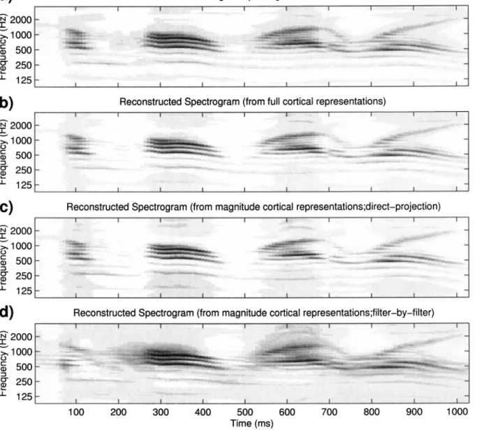
within the effective band can be obtained. One example is shown in Fig. 9共b兲 with the rates up to 32 Hz and scales up to 8 cycles/ octave used in the reconstruction. The recon-structed signals can be heard at http://www.isr.umd.edu/ CAAR/pubs.html.
It is likely that temporal modulations faster than 20– 40 Hz are encoded in the auditory cortex only by their energy distribution or envelope rather than by their actual phase-locked waveforms 共Kowalski et al., 1996; Lu et al., 2001兲. Psychoacoustic experiments and previous models of temporal modulation sensitivity also support this conclusion 共Dau et al., 1997b; Sheft and Yost, 1990兲. Furthermore, in certain applications of the cortical model共Chi et al., 1999兲, the output magnitude turns out to be an efficient and excel-lent indicator of the information and percepts of the stimulus. It is therefore useful to demonstrate that the “magnitude” of the response carries sufficient information about the stimulus that generated it. In the Appendix, two algorithms are pro-posed to reconstruct original speech from the modulation-energy-distributions关兩z⇓兩 and 兩z⇑兩 in Eqs. 共16兲 and 共17兲兴 only. While the “quality” of the reconstructed signals is worse due to a smaller dynamic range or to propagation of errors in the
reconstruction procedures共see the Appendix兲, they are com-pletely intelligible as can be heard on the website http:// www.isr.umd.edu/CAAR/pubs.html.
C. Quality of the reconstructed speech signals
The multiscale auditory model共together with its recon-struction algorithms兲 can be essentially considered a “coding-decoding” system, and as such we can derive an objective assessment of the “quality” of the reconstructed speech by comparing it to the original clean samples using the standard perceptual evaluation of speech quality共PESQ兲 metric recommended by ITU 共ITU-T, 2001兲. In this model-based method, we compare samples of clean speech signals to samples reconstructed from the auditory spectrogram and the full cortical representation 共magnitude and phase in-cluded兲. The typical PESQ score obtained for the reconstruc-tion from the auditory spectrogram is 4+ 共toll quality兲. For instance, the average of 50 reconstructions of the sentence /Come home right away/共Fig. 9兲 starting from different ini-tial conditions and after 200 iterations is 4.04 with = 0.075. The average PESQ score for the reconstruction from
FIG. 8. Two examples of reconstructed acoustic waves from auditory spectrograms:共a兲 sentence /I honor my mom/ spoken by a male speaker and 共b兲 sentence /Leave me your address/ spoken by a female speaker. The original speech signals are extracted from TIMIT corpus. In each example, the original time waveform关s共t兲兴, the target auditory spectrogram 关yfinal共t,x兲兴, the reconstructed time waveform 关s˜共t兲兴, and the corresponding auditory spectrogram 关y˜final共t,x兲兴
the full cortical representation 共with rates up to 128 Hz and scales up to 8 cycles/ octave兲 is 4.02 共toll quality兲 with = 0.069.
D. Intelligibility of the reconstructed signals
To demonstrate the utility of the reconstructed speech signals from the model, we explore the assertions we made earlier in the Introduction regarding the critical role played by the slow spectrotemporal envelope modulations in pre-serving intelligibility of the speech signal. Specifically, we use the model to reconstruct a speech sentence after remov-ing from its original version progressively more of its tem-poral and spectral modulations. We assess in psychoacoustic tests the perceptual effect of such manipulations, and com-pare the results to the spectrotemporal modulation index 共STMI兲, a measure that was previously demonstrated to be a reliable correlate of human perception of speech intelligibil-ity under a wide variety of interference signals and
condi-tions 共Elhilali et al., 2003兲. We shall specifically employ a particular version of the STMI denoted by STMIT共Elhilali et al., 2003兲, where the superscript “T” refers to the use of a
clean speech signal as the “template” to be compared to each of the “modulation reduced” 共or distorted兲 versions recon-structed from the model.
We first compute the multiscale representation of the clean speech signal through the model 关as in Eqs. 共16兲 and 共17兲, ∀c兴. Temporal modulations are then filtered out by nulling the outputs of the undesired filters共parametrized by their center modulation ratescand⍀c兲. This “filtered”
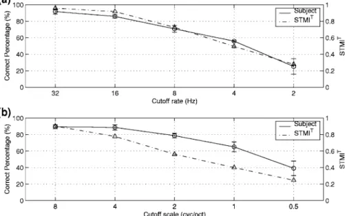
rep-resentation is then inverted to reconstruct the corresponding “modulation reduced” acoustic signal 共as explained in Sec. V B兲. Figure 10共a兲 shows the STMIT of the reconstructed speech as a function of the upper limit of temporal modula-tion rates共dashed line兲. Rates along the abscissa refer to the c’s of the cortical filters that are nulled in the STMIT
com-putations. Since the filters are fairly broad, these rates are
FIG. 9. Examples of reconstructed spectrograms. The top panel shows the original spectrogram of sentence /Come home right away/ spoken by a male speaker. The reconstructed spectrograms from full cortical representations and magnitude cortical representations共direct-projection and filter-by-filter algo-rithms兲 are demonstrated on the second to bottom panel, respectively. All spectrograms are reconstructed from those cortical representations which only include modulation rates up to 32 Hz.
gradual. Each value of the STMIT shown in the plot is the average of 20 sentences 共a mix of males and females兲 ex-tracted from the TIMIT corpus 共the training portion of the New England dialect region兲. It is evident that intelligibility becomes marginal when temporal modulations around 4 Hz are filtered out, consistent with numerous previous experi-mental results 共Elhilali et al., 2003; Drullman et al., 1994兲. These results are consistent with the average intelligibility scores measured with four native speakers. In these tests, each subject was to identify 300 reconstructed CVC word samples 关see Elhilali et al. 共2003兲 for experiment details兴. The average percentage “correct phonemes” and the error bars with one standard deviation ranges are plotted in Fig. 10共a兲.
Figure 10共b兲 illustrates the STMIT and intelligibility scores obtained when the spectral profiles of the speech sen-tence are smoothed by removing progressively higher scales. While the STMIT and subjects’ performance deviate from each other, the overall results confirm that the loss of spec-trally sharp features diminishes intelligibility gradually be-ginning when the filters are effectively wider than about the critical bandwidth共3 cycles/octave兲. Some intelligibility re-mains even with filters as broad as 0.5– 1 cycles/ octave共or about an octave兲, consistent with previous experimental find-ings共Shannon et al., 1995兲.
VI. DISCUSSION
We presented a model of auditory processing that trans-forms an acoustic signal into a multiresolution spectrotem-poral representation inspired by experimental findings from the auditory cortex. The model consists of two major trans-formations of the acoustic signal:
共1兲 A frequency analysis stage associated with the cochlea, cochlear nucleus, and response features observed in the midbrain: This stage effectively computes an affine wavelet transform of the acoustic signal with a spectral resolution of about 10%共Lyon and Shamma, 1996兲.
共2兲 A spectrotemporal multiresolution analysis stage postu-lated to conclude in the primary auditory cortex: This stage effectively computes a two-dimensional affine wavelet transform with a Gabor-like spectrotemporal mother-wavelet关see Fig. 5共b兲兴.
The model is intended to be a computational realization of the most basic aspects of auditory processing and not a biophysical description of its stages. Hence, there is only a loose correspondence between any specific structure and model parameters. However, we hypothesize that the model final representation of the acoustic signal captures explicitly and quantitatively the spectral and dynamic aspects that are directly perceived by a listener. Consequently, this represen-tation may be utilized to account for a variety of phenomena, especially those related to the perception of timbre, such as in the assessment of speech quality and intelligibility 共El-hilali et al., 2003; Chi et al., 1999兲, discrimination of musical timbre 共Ru and Shamma, 1997兲, and, more generally, quan-tifying the perception of complex sounds subjected to arbi-trary spectral and temporal changes 共Carlyon and Shamma, 2003兲.
The spirit of this model shares much with others that have been proposed to quantify the perceptual relevance of temporal modulations in acoustic signals共Dau et al., 1997a; Sheft and Yost, 1990; Houtgast, 1989; Bacon and Grantham, 1989; Viemeister, 1979兲. Dau and colleagues developed the most detailed of these models, consisting of a bank of purely temporal modulation selective filters. They also established its parameters and perceptual relevance in a series of exten-sive psychoacoustic experiments共Dau et al., 1997a b兲. Our model is consistent with Dau’s model in the details of its analysis of temporal modulations, e.g., possessing similar fil-ter bandwidths in the modulation filfil-terbank 共Q3dB= 1.8 ver-sus Q3dB= 2 in Dau’s model兲. The two models fundamentally differ in the way temporal modulations from different spec-tral channels are integrated at the end. Dau’s model is fully
separable, integrating spectral information subsequent to an
independent temporal analysis. By contrast the multiscale
FIG. 10. The spectro-temporal modulation index共STMIT兲 共Elhilali et al., 2003兲 of
re-constructed speech as a function of the range of spectral and temporal modulations pre-served in the signal.共a兲 The STMIT共dashed
line兲 and the experimental measurements of the correct phoneme recognition percentage of human subjects共solid line兲 as a function of the range of temporal modulations pre-served.共b兲 The STMIT共dashed line兲 and the
human performance共solid line兲 as function of the scales preserved.
cortical model is inseparable共but see footnote 3兲, postulating a “spectral” modulation filterbank that is fully integrated with the temporal modulation analysis. Under circumstances where both temporal and spectral features of the input spec-trograms are manipulated 关e.g., as in phase jitter or phase shift distortions described in Elhilali et al. 共2003兲兴, the two models respond differently.
A. Variations on the cortical model
As with the early auditory stage, the multiresolution cor-tical model is highly schematic and lacks realistic biophysi-cal mechanisms and parameters. Nevertheless, the model aims to capture perceptually significant features in the audi-tory spectrogram, and hence justify its relevance through its successful application in accounting for a variety of percep-tual thresholds and tasks as we have described above.
Many details of the model are somewhat arbitrary and can be probably modified to reflect future physiological and anatomical findings with no significant effect on the compu-tations. For example, real cortical STRFs 共Fig. 1兲 are far more complex than the simple Gabor-like shapes we have employed in the model. They are often tuned to multiple frequencies and are rarely purely selective to upward or downward frequency sweeps but rather are simply more re-sponsive to one direction or the other. In many situations, these differences are not crucial as long as important spec-trogram features共e.g., FM sweeps and AM modulations兲 are still encoded explicitly albeit in a different form.
One potentially interesting variation on our model is to split the spectrotemporal modulation analysis into two stages. The first would be a relatively fast bank of filters mimicking the temporal analysis hypothesized to exist in the inferior colliculus 共Langner and Schreiner, 1988兲 共rates of 30– 1000 Hz兲. The second stage would be slower filters 共艋30 Hz兲 operating on each output from the earlier stage. This latter stage would then capture all the important slow modulations of the spectrogram explicitly, whereas the ear-lier stage extracts the intermediate and fast modulations of the auditory spectrogram. The natural split between the dy-namic factors involved in intelligibility共the slow rates found in the cortex兲 from those involved in sound quality 共interme-diate rates found precortically兲 becomes particularly advan-tageous when considering phenomena that contrast these two rate domains such as the streaming of two sounds based purely on their modulation rates共Roberts et al., 2002; Gri-mault et al., 2002兲.
B. Relation to previous reconstruction algorithms The multiresolution representation and associated recon-struction algorithms presented here differ from previous methods for processing spectral and temporal envelopes in two ways. First, its formulation combines the spectral and temporal dimensions compared to the purely spectral 共e.g., ter Keurs et al., 1992; Baer and Moore, 1993兲, purely tem-poral共e.g., Drullman et al., 1994兲, or a separable cascade of the two共e.g., Dau et al., 1997b兲. Second, our reconstruction algorithm starts from a random noise signal without any prior information about the original speech. By contrast,
pre-vious experiments usually retained the carrier waveform of the speech in each frequency band共Drullman et al., 1994兲 or the harmonic structure of the speech in each frame共ter Keurs
et al., 1992; Baer and Moore, 1993兲 and used them to
resyn-thesize the filtered speech by superimposing the newly pro-cessed envelopes upon them. These carriers improve the quality of the reconstructed speech, but may contain residual intelligible information共Ghitza, 2001; Smith et al., 2002兲.
Our algorithms are similar in spirit to Slaney’s inversion algorithm 共Slaney et al., 1994兲, which also employs the it-erative projection method and disposes of the fine structure in reconstructing the stimulus. The algorithm, however, dif-fers fundamentally in all of its details in that it uses for its two-stage representation the cochleagram from a simpler Gammatone filter bank cochlear model 共as opposed to the
early stage兲 and the correlogram 共as opposed to the cortical multiscale representation兲. Consequently, all the constraints
imposed during the iterations are completely different.
C. Applications of the multiscale auditory model The validity of the auditory model stems from its ability to account for psychoacoustic findings and from its success-ful application in a variety of perceptual tasks. To this end, we have recently adapted and tested the auditory model in several very different contexts. In the first, the auditory model was used to account for the detection of phase of complex sounds such as phase differences between the enve-lopes of sounds occupying remote frequency regions, and between the fine structures of partials that interact within a single auditory filter共Carlyon and Shamma, 2003兲. The ap-proach was simply to interpret the discrimination between two stimuli as being proportional to the distance 共or differ-ence兲 measured between their cortical representation in the model 共Tchorz and Kollmeier, 1999兲. Discriminations suc-cessfully accounted for phase differences between pairs of bandpass filtered harmonic complexes, and between pairs of sinusoidally amplitude modulated tones, discrimination be-tween amplitude and frequency modulation, and discrimina-tion of transient signals differing only in their phase spectra 共“Huffman sequences”兲 共Carlyon and Shamma, 2003兲.
In a second application, we used the model to analyze the effects of noise, reverberations, and other distortions on the joint spectrotemporal modulations present in speech, and on the ability of a channel to transmit these modulations共Chi
et al., 1999; Elhilali et al., 2003兲. The rationale behind this
approach is that the perception of speech is critically depen-dent on the faithful representation of spectral and temporal modulations in the auditory spectrogram 共Hermansky and Morgan, 1994; Drullman et al., 1994; Shannon et al., 1995; Arai et al., 1996; Dau et al., 1996; Greenberg et al., 1998兲. Therefore, an intelligibility index which reflects the integrity of these modulations can be effective regardless of the source of the degradation. Such a spectrotemporal modula-tion index 共STMI兲 was derived using the model representa-tion of speech modularepresenta-tions and was validated by comparing its predictions of intelligibility to those of the classical
speech transmission index (STI) and to error rates reported