Short Paper
_________________________________________________Machine Learning with Automatic Feature Selection
for Multi-class Protein Fold Classification
*CHUEN-DER HUANG+, SHENG-FU LIANG, CHIN-TENG LIN AND RUEI-CHENG WU
+
Department of Electrical Engineering Hsiuping Institute of Technology
Taichung, 412 Taiwan
Department of Electrical and Control Engineering National Chiao Tung University
Hsinchu, 300 Taiwan E-mail: ctlin@mail.nctu.edu.tw
In machine learning, both the properly used networks and the selected features are important factors which should be considered carefully. These two factors will influence the result, whether for better or worse. In bioinformatics, the amount of features may be very large to make machine learning possible. In this study we introduce the idea of feature selection in the problem of bioinformatics. We use neural networks to complete our task where each input node is associated with a gate. At the beginning of the training, all gates are almost closed, and, at this time, no features are allowed to enter the network. During the training phase, gates are either opened or closed, depending on the requirements. After the selection training phase has completed, gates corresponding to the helpful features are completely opened while gates corresponding to the useless features are closed more tightly. Some gates may be partially open, depending on the importance of the corresponding features. So, the network can not only select features in an online manner during learning, but it also does some feature extraction. We combine feature selection with our novel hierarchical machine learning architecture and apply it to multi-class protein fold classification. At the first level the network classifies the data into four major folds: all alpha, all beta, alpha + beta and alpha/beta. In the next level, we have another set of networks which further classifies the data into twenty-seven folds. This approach helps achieve the following. The gating network is found to reduce the number of features drastically. It is interesting to observe that, for the first level using just 50 features selected by the gating network, we can get a test accuracy comparable to that using 125 features in neural classifiers. The process also helps us get a better insight into the folding process. For example, tracking the evolution of different gates, we can find which characteristics (features) of the data are more important for the folding process. Eventually, it reduces the computation time. The use of the hierarchical architecture helps us get a better performance also.
Keywords: machine learning, hierarchical architecture, feature selection, gate, neural
network, protein fold, bioinformatics
Received June 3, 2003; revised March 24 & June 1, 2004; accepted July 15, 2004. Communicated by Chuen-Tsai Sun.
1. INTRODUCTION
For the past few decades, neural networks (NNs) had been used as an intelligent machine learning method in many fields such as pattern recognition, speech and bioinformatics. There have been several attempts to use NNs for the prediction of protein folds.
Dubchak et al. [1] pointed out that when they requested a broad structural classi- fication of protein, four classes, all alpha, all beta, (alpha + beta) and (alpha/beta), it was easy to get more than 70% prediction accuracy using a simpler feature vector to represent a protein sequence [2-4]. However, the problem become more and more difficult as demand for more classes increased.
Dubchak et al. [5] used a multi-layer perceptron network for predicting protein folds using global description of the chain of amino acids to represent proteins. They used the different properties of amino acids as features. For example, they used the relative hydrophobicity of amino acids and also used information about the predicted secondary structure and the predicted solvent accessibility. With this method, they divided the amino acids into the following: three groups based on the hydrophobicity, three groups based on secondary structure and four groups based on the solvent accessibility. Now, a protein sequence is described based on three global descriptors: Composition (C), Transition (T) and Distribution (D). These descriptors essentially describe the frequencies with which the properties change along the sequence and their distribution on the chain. In reference [5], the authors used various combinations of these features and trained networks to find a good set of features.
Dubchak et al. [1] proposed a neural network-based scheme for classifying protein folds into 27 classes. This method, as the one in reference [5], used global descriptors of the primary sequence. These descriptors were also computed from the physical, chemical and structural properties of the constituent amino acids.
In reference [1], the authors used proteins from the PDB where two proteins had no more than 35% of sequence identity. Here, in addition to the three amino acid attributes described earlier, the authors used three more attributes: normalized van der Walls volume, polarity and polarizability. The same set of descriptors were used for all attributes resulting in a parameter vector of 21 components for each attribute. They also used the percent composition of amino acids as feature vectors. Let there be M folds in the data set. For each fold, the authors divided the data set into two groups, one containing points from the fold and the other containing the rest. So, there were M such partitions. For each fold an NN is trained. This procedure was repeated seven times for each fold. Each time only one set of features computed from a particular attribute was used and this procedure was repeated seven times for each fold. Then, a voting mechanism was used to decide the fold of a given protein. All these investigations clearly suggest that features are very important for a better prediction of protein folds.
Researchers in bioinformatics have acknowledged the importance of feature analysis. Some systematic efforts to find the best set of features have been done. But mostly, the authors have used enumeration techniques. Feature analysis is more important for bioinformatics applications for two reasons: the class structure is highly complex and the data usually has very large dimensions. Most of the feature analysis
techniques available in the pattern recognition literature are off-line in nature. It is known that every feature,which characterizes a data point may not have the same impact with regard to its classification, i.e., some features may be redundant and some may have derogatory influence on the classification task. Thus, selection of a proper subset of features from those available is important for the design of efficient classifiers. There are methods for selecting good features based on feature ranking, etc., [6-9].
The goodness of a feature depends on the problem being solved and on the tools being used to solve the problem [6]. Therefore, feature selection, can select the most appropriate features for the task and result in a good classifier simultaneously. In referecne [10], Pal et al. developed an integrated feature selection and classification scheme based on the multilayer perceptron architecture. We would like to use the same concept here to reduce the dimensionality of the data. In addition to this, we use a novel hierarchical architecture for achieving a better classification performance [5].
2. ONLINE FEATURE SELECTION THROUGH GATING
In a standard multilayer perceptron network, the effect of some features (inputs) can be eliminated by forbidding them to enter the network, i.e., by equipping each input node (hence each feature) with a gate and closing the gate. For good features, the associated gates can be completely opened. On the other hand, if a feature is partially important, then, the corresponding gate should be partially opened. Pal and Chintalapudi [10] suggested a mechanism for realizing such a gate so that “partially useful” features are identified and attenuated according to their relative usefulness. In order to model the gates, we consider an attenuation function for each feature such that, for a good feature, the function produces a value of 1 or nearly 1, while for a bad feature, the value should be nearly 0. For a partially effective feature, the value should be intermediate in value. To model the gate, we multiply the input feature value by its gate function value and the modulated feature value is passed into the network. The gate functions attenuate the features before they propagate through the net, so we may call these gate functions attenuation functions. A simple way of identifying useful gate functions is to use sigmoidal functions with a tunable parameter, which can be learned by using training data. To complete the description of the method, we define the following in connection with a multi-layer perceptron network.
Let Fi : R → [0, 1] be the gate or attenuation function associated with the ith input feature; Fi has an argument wi; Fi′(wi) is the derivative of the attenuation function at wi; µ is the learning rate of the attenuation parameter; i is the learning rate of the connection weights; xi is the ith input of an input vector; x′ is the attenuated value of x, i.e., x′ = xF(w);
0
ij
w is the weight connecting the jth node of the first hidden layer to the ith node of the input layer; and δ1j is the error term for the j-th node of the first hidden layer. It can be
easily shown that, except for wij0, the update rules for all weights remain the same as that for an ordinary MLP. Assuming that the first hidden layer has q nodes the update rules
for w and wij0 i are
0 0 1
, , ( ),
ji new ji old i j i
0 1 , , 1 ( ) ( ). q i new i old i ji j i j w w µx w δ F w = ′ = −
∑
(2) Although for the gate function, several choices are possible, here we use the sigmoidal function F(w) = 1.0/(1 + e−w). The p gate parameters are initialized so that when the training starts, F(w) is practically zero for all gates, i.e., no feature is allowed to enter the network. As the back-propagation learning proceeds, gates for the features that can reduce the error faster are opened. Note that, the learning of the gate function continues along with other weights of the network. At the end of training, the important features can be picked up based on the values of the attenuation function.3. LEARNING MACHINES
In our experiment, we use a novel hierarchical learning architecture which has been proposed by us [11]. The concept of the hierarchical architecture is neither the same as the cascade network nor the divide-and-conquer network. The constituents of the hierarchical architecture are all independent networks.
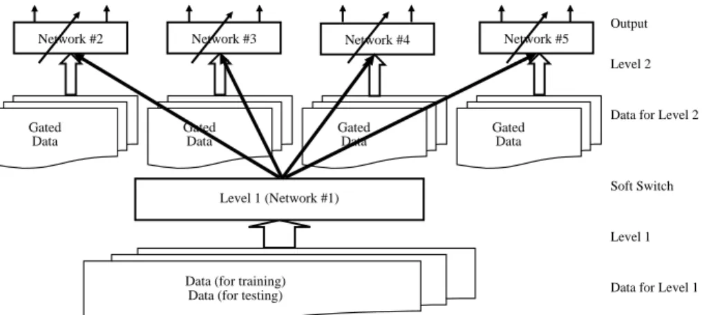
A hierarchical architecture is suitable for data sets that can be grouped into a smaller number of classes, where each class can be further divided into a set of other classes. The problem handled here, the multi-classification of protein structure, has this characteristic. Under each of the main structures, all alpha, all beta, alpha/beta and alpha + beta, there are several folds. Fig. 1 illustrates the concept of hierarchical learning architecture.
Gated Data Gated Data Gated Data Gated Data Network #2 Level 1 (Network #1) Network #4 Network #5
Data (for training) Data (for testing)
Network #3
Output
Level 2
Data for Level 2
Soft Switch
Level 1
Data for Level 1
Fig. 1. Concept of hierarchical learning architecture. In the figure, the black solid arrows between levels 1 and 2 are soft switchs used to switch the classified data of level 1 to corresponding classifiers of level 2.
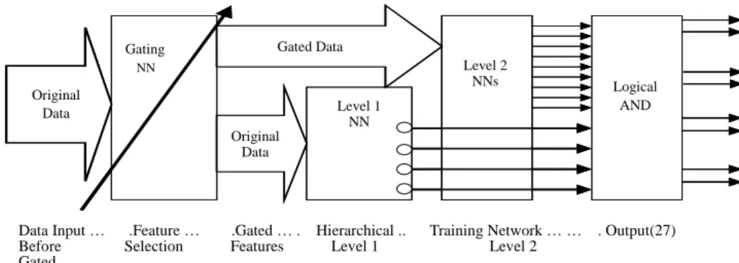
Before training the hierarchical classifier, data should be passed through the feature selection network to find the important features. Fig. 2 shows the integrated view of the whole system. There are major components, the gating network and the hierarchical classifier. First, the original data is used to train the gating network. At the end of the
G a t i n g N N L e v e l 1 N N L e v e l 2 N N s L o g i c a l A N D O r i g i n a l D a t a G a t e d D a t a G a t e d D a t a D a t a I n p u t … . F e a t u r e … . G a t e d … . H i e r a r c h i c a l . . T r a i n i n g N e t w o r k … … . O u t p u t ( 2 7 ) B e f o r e S e l e c t i o n F e a t u r e s L e v e l 1 L e v e l 2 G a t e d G a t i n g N N L e v e l 1 N N L e v e l 2 N N s L o g i c a l A N D O r i g i n a l D a t a G a t e d D a t a G a t e d D a t a D a t a I n p u t … . F e a t u r e … . G a t e d … . H i e r a r c h i c a l . . T r a i n i n g N e t w o r k … … . O u t p u t ( 2 7 ) B e f o r e S e l e c t i o n F e a t u r e s L e v e l 1 L e v e l 2 G a t e d Original Data Gated Data Original Data Level 1 NN Level 2 NNs Logical AND Gating NN
Data Input … .Feature … .Gated … . Hierarchical .. Training Network … … . Output(27) Before Selection Features Level 1 Level 2
Gated
Fig. 2. Block diagram of overall learning system. In the architecture, features are gated by a gate before they are fed into classifiers. The gated data feed into levels 1 and 2 are the same data sets which have been gated. By using gated data, the classifiers can do its mission, four outputs for level 1 and 27 for level 2.
training, we look at the gate function values for each feature. If the gate function value is greater a threshold th, then we consider that feature important. In this way, from the initial set of p features, we get a reduced set of q important features.
Now, this q-dimensional data set is used to train the hierarchical learning machine represented by Levels 1 and 2 in Fig. 1. This hierarchical machine is shown in Fig. 2. Let the training data be XTr = X1∪ X2∪ X3∪ X4, where Xi is the training data corresponding to group i. First, we train the Level 1 NN (the NN in Level 1, see Fig. 1) using X. The Level 1 NN divides the data into four groups. Note that the division of X made by the Level 1 NN may not exactly correspond to XTr = X1 ∪ X2 ∪ X3 ∪ X4. The Level 2 networks are independently trained. The ith Level 2 NN is trained with Xi. Once the training of the second level networks is complete, the system is ready to be tested. A test data point is first passed through the gating network, which reduces its dimension to q. This q dimensional data point is now fed to the Level 1 NN which will classify the point to one of the four groups, say to group 3. Then, the training data point is fed to the 3rd network in the second level. It should be noted here that, for such an architecture, if the Level 1 NN makes any mistakes, the Level 2 network cannot recover the same. The proposed architecture is quite general and, hence, for both Levels 1 and 2, we can use any classification network In fact, we can use any non-neural classifier too. Although features are selected by using a feature-selection multilayer perceptron type network, we use the selected features for classification by using both MLP and RBF networks.
4. DATA SET AND FEATURES
For bioinformatics applications, feature extraction is a very important task which deserves discussion because the extracted features may have a strong influence on the accuracy. Table 1 summarizes the characteristics of the descriptors. For comparison, we used the same data sets as Dubchak and Ding’s prior work. The number of training proteins used in our experiments is 313. They can be divided into 4 groups with 27 folds.
Table 1. Features used in the experiments.
Descriptors Features
Composition (C) 20 kinds of amino acids 20
Predicted Secondary Structure (S) Alpha Beta Loop 21
Hydrophobicity (H) Positive Neutral Negative 21
Volume (V) Large Middle Small 21
Polarity (P) Positive Neutral Negative 21
Polarizability (Z) Strong Middle Weak 21
Total 125
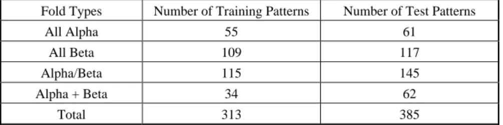
Table 2. Numbers of patterns in the training and test sets.
Fold Types Number of Training Patterns Number of Test Patterns
All Alpha 55 61
All Beta 109 117
Alpha/Beta 115 145
Alpha + Beta 34 62
Total 313 385
The number of proteins used in the test set is 385. Table 1 shows the number of input nodes of the neural networks. Table 2 depicts the distribution of training and test proteins in different groups.
5. EXPERIMENTS AND RESULTS
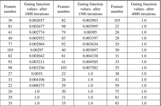
We have run the gating networks for several times and the results presented correspond to some typical outputs. We emphasize the fact that, depending on the initialization, two different sets of features may be picked by the gating net as the important items in two different runs. This is absolutely fine, as features are often highly correlated. Moreover, depending on the choice of threshold, the number of selected features may be different. Table 3 shows 15 of the most important features of a typical run of the gating network after 1000, 1500, and 4000 iterations. It is interesting to note that, after 1000 iterations, eight of the top-most 15 important features come from the group predicted by the secondary structure. Of these eight, one of the features, No. 27, disappears from the list of important features with further iterating. Probably, the gate corresponding to some other correlated feature opened faster.
After 4000 iterations, of the 15 important features, nine come from the predicted secondary structure. This clearly tells that the local secondary structure, as expected, has a strong impact on the final folds. In this list of 15 important features, we have representation from polarity, polarizability, volume and hydrophobicity. In this investigation, we initialized the gating function with a value of 0.000124.
Table 3. Values of the gate functions for the most important 15 features after different numbers of iterations. Feature number Gating function values- after 1000 iterations Feature number Gating function values- after 1500 iterations Feature number Gating function values- after 4000 iterations 30 0.002657 82 0.002903 103 1.0 81 0.002677 98 0.002995 22 1.0 41 0.002774 79 0.00305 26 1.0 40 0.002952 83 0.003197 28 1.0 77 0.002964 92 0.003634 29 1.0 103 0.00297 40 0.003697 30 1.0 82 0.003042 81 0.004338 31 1.0 92 0.003211 41 0.004585 33 1.0 98 0.003256 103 0.007582 35 1.0 27 0.0035 22 1.0 38 1.0 31 0.004106 26 1.0 41 1.0 22 0.008275 29 1.0 59 1.0 26 1.0 30 1.0 75 1.0 29 1.0 31 1.0 81 1.0 35 1.0 35 1.0 83 1.0
Table 4. Performance of ordinary MLP on different subsets of features.
C CS CSH CSHP CSHPV CSHPVZ Correct Classifications 243 (63.1%) 308 (80.0%) 305 (79.2%) 301 (78.2%) 302 (78.4%) 309 (80.3%)
Table 4 depicts the classification performance at level 1 (into four groups) by the MLP network with different sets of features. Table 4 reveals that the use of more features are not necessarily good. It also says that the distribution predicted secondary structure and composition constitute a good set of features. This is also consistent with the results obtained from the gating network.
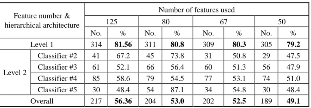
Table 5 presents classification performance of the system with different feature sets when RBF nets are used as the basic classifier unit. The Level 1 performance shows that, with 67 features (50% reduction), the decrease in performance is only 1.26%, while with 65% of the features, the test accuracy is reduced by only 0.76%. This clearly suggests that the gating network can do an excellent job in selecting important features. Let us consider the overall classification performance (with 27 folds) now. For this case, we get 53% of the test accuracy with 67% of the features which is just 3% less than what we can achieve in taking all 125 featues into account. Comparing our results with that of Dubchak et al. [12], we find that All vs. All method with support vector machines they used can result in a test accuracy of 53.9%, while with the RBF networks, using only 67% of the features, we can get 53% of the test accuracy.
Table 5. Performance of the hierarchical system using different feature gated sets.
Number of features used
125 80 67 50
Feature number & hierarchical architecture
No. % No. % No. % No. %
Level 1 314 81.56 311 80.8 309 80.3 305 79.2 Classifier #2 41 67.2 45 73.8 31 50.8 29 47.5 Classifier #3 61 52.1 66 56.4 60 51.3 56 47.9 Classifier #4 85 58.6 79 54.5 77 53.1 74 51.0 Level 2 Classifier #5 30 48.4 54 87.1 34 54.8 30 48.4 Overall 217 56.36 204 53.0 202 52.5 189 49.1 6. CONCLUSIONS
In this paper, we integrated two novel ideas: an online feature selection technique and a hierarchical learning machine to treat the multi-class protein fold recognition problem. The results show that the proposed architecture is quite effective in both reducing the dimensionality of the data and enhancing the classification performance.The proposed methods are simpler than other machine learning methods, e.g. one-vs.-others method. Since the consideration of all possible subsets is not computatonally feasible, it is often impossible to find the best set of features. The proposed technique allows the processing of more futures from amino acid sequences, such as N-gram and spaced-N- gram. We have used these high-order features along with the features used in this paper in our experiemnts and have achieved higher accuracy than other exisitng methods.
REFERENCES
1. I. Dubchak, I. Muchnik, C. Mayor, I. Dralyuk, and S. H. Kim, “Recognition of a protein fold in the context of the SCOP classification,” PROTEINS: Structure,
Function and Genetics, Vol. 35, 1999, pp. 401-407.
2. P. Y. I. Chou and G. D. Fashman, (eds.), Prediction of Protein Structure and
Principles of Protein Conformation, Plenum Press, New York, 1989, pp. 549-586.
3. H. Nakashima, K. Nishikawa, and T. Ooi, “The folding type of a protein is relevant to the amino acid composition,” Journal of Biochem, Vol. 99, 1986, pp. 152-162. 4. I. Dubchak, S. R. Holbrook, and S. H. Kim, “Prediction of protein folding class from
amino acid composition,” Proteins, Vol. 16, 1993, pp. 79-91.
5. I. Dubchak, I. Muchnik, S. R. Holbrook, and S. H. Kim, “Prediction of protein folding class using global description of amino acid sequence,” in Proceeding of
National Academia (Biophysics), Vol. 92, 1995, pp. 8700-8704.
6. R. De, N. R. Pal, and S. K. Pal, “Feature analysis: neural network and fuzzy set theoretic approaches,” Pattern Recognition, Vol. 30, 1997, pp. 1579-1590.
7. K. Fukunaga and W. Koontz, “Applications of the karhunen-loeve expansion to feature selection and ordering,” IEEE Transactions on Computers, Vol. C-19, 1970, pp. 311-318.
8. K. L. Priddy, S. K. Rogers, D. W. Ruck, G. L. Tarr, and M. Kabrisby, “Bayesian selection of important features for feed-forward neural network,” NeuroComputing, Vol. 5, 1993, pp. 91-103.
9. A. Verikas and M. Bacauskiene, “Feature selection with neural networks,” Pattern
Recognition Letters, Vol. 23, 2002, pp. 1323-1335.
10. N. R. Pal and K. Chintalapudi, “Connectionist system for feature selection,” Neural,
Parallel and Scientific Computation, Vol. 5, 1997, pp. 359-381.
11. I. F. Chung, C. D. Huang, Y. H. Shen, and C. T. Lin, “Recognition of structure classification of protein folding by NN and SVM hierarchical learning architecture,”
International Conference on Neural Information Processing (ICONIP ’03), 2003,
pp. 1159-1167.
12. I. Dubchak and C. H. Q. Ding, “Multi-class protein fold recognition using support vector machines and neural networks,” Bioinformatics, Vol. 17, 2001, pp. 349-358.
Chuen-Der Huang (黃淳德) received the B.S. degree in Electrical Engineering in 1980 and M.S. degree in Automatic Control Engineering in 1983 both from Feng Chia University, Taichung, Taiwan. He received the Ph.D. degree in the Department of Elec-trical and Control Engineering, National Chiao Tung University, Hsinchu, Taiwan. Dr. Huang currently serves as an Associate Professor in the Department of Electrical Engi-neering, HsiuPing Institute of Technology, Taichung, Taiwan. Dr. Huang also as the Di-rector of the Affiliated Institute of Continuing Education of HsiuPing Institute of Tech-nology currently. His research interests include bioinformatics, machine learning, fuzzy control, automation, and data mining.
Sheng-Fu Liang (梁勝富) was born in Tainan, Taiwan, in 1971. He received the B.S. and M.S. degrees in Control Engineering from the National Chiao Tung University (NCTU), Taiwan, in 1994 and 1996, respectively. He received the Ph.D. degree in Elec-trical and Control Engineering from NCTU in 2000. Currently, he is a Research Assistant Professor in Electrical and Control Engineering, NCTU. Dr. Liang has also served as the executive secretary of Brain Research Center, NCTU Branch, University System of Tai-wan since September 2003. His current research interests are neural networks, fuzzy neu-ral networks (FNN), brain-computer interface (BCI), and multimedia signal processing.
Chin-Teng Lin (林進燈) received the B.S. degree in Control Engineering from the National Chiao Tung University, Hsinchu, Taiwan, in 1986 and the M.S. and Ph.D. de-grees in Electrical Engineering from Purdue University, U.S.A., in 1989 and 1992, re-spectively. Since August 1992, he has been with the College of Electrical Engineering and Computer Science, National Chiao Tung University, Hsinchu, Taiwan, where he is currently the Associate Dean of the college and a professor of Electrical and Control En-gineering Department. He served as the Director of the Research and Development Of-fice of the National Chiao Tung University from 1998 to 2000, and the Chairman of Electrical and Control Engineering Department from 2000 to 2003. His current research interests are neural networks, fuzzy systems, cellular neural networks (CNN), fuzzy
neu-ral networks (FNN), VLSI design for pattern recognition, intelligent control, and multi-media (including image/video and speech/audio) signal processing, and intelligent transportation system (ITS). He is the book co-author of Neural Fuzzy Systems − A
Neuro-Fuzzy Synergism to Intelligent Systems (Prentice Hall), and the author of Neural Fuzzy Control Systems with Structure and Parameter Learning (World Scientific). Dr.
Lin is a member of Tau Beta Pi, Eta Kappa Nu and Phi Kappa Phi honorary societies. He is also a member of the IEEE Circuit and Systems Society (CASS), the IEEE Neural Network Society, the IEEE Computer Society, the IEEE Robotics and Automation Soci-ety, and the IEEE System, Man, Cybernetics Society. Dr. Lin is also the member and Secretary of Neural Systems and Applications Technical Committee (NSATC) of IEEE CASS and will join the Cellular Neural Networks and Array Computing (CNNAC) Technical Committee soon. Dr. Lin is the Distinguished Lecturer representing the NSATC of IEEE CASS from 2003 to 2004. Dr. Lin has been the Executive Council member (Supervisor) of Chinese Automation Association since 1998. He was the Execu-tive Council member of the Chinese Fuzzy System Association Taiwan (CFSAT), from 1994 to 2001. Dr. Lin is the Society President of CFSAT since 2002. He was the Chair-man of IEEE Robotics and Automation Society, Taipei Chapter from 2000 to 2001. Dr. Lin has won the Outstanding Research Award granted by National Science Council (NSC), Taiwan, since 1997 to present, the Outstanding Electrical Engineering Professor Award granted by the Chinese Institute of Electrical Engineering (CIEE) in 1997, the Outstanding Engineering Professor Award granted by the Chinese Institute of Engineer-ing (CIE) in 2000, and the 2002 Taiwan OutstandEngineer-ing Information-Technology Expert Award. Dr. Lin was also elected to be one of the 38th Ten Outstanding Rising Stars in Taiwan, (2000). Dr. Lin currently serves as the associate editors of IEEE Transactions on Systems, Man, Cybernetics (Part B), IEEE Transactions on Fuzzy Systems, International Journal of Speech Technology, and the Journal of Automatica. He is a Senior Member of IEEE.
Ruei-Cheng Wu (吳瑞成) received the B.S. degree in Nuclear Engineering from National Tsing Hua University, Taiwan, R.O.C., in 1995, and M.S. degree in Control Engineering from National Chiao Tung University, Taiwan, in 1997. He is currently pur-suing the Ph.D. degree in brain research center in electrical and control engineering at National Chiao Tung University, Taiwan. His current research interests are brain re-search, audio signal processing, fuzzy control, neural networks, and linear control sys-tem.