American Society for Quality
Adding a Variable in Generalized Linear Models Author(s): P. C. Wang
Source: Technometrics, Vol. 27, No. 3 (Aug., 1985), pp. 273-276
Published by: American Statistical Association and American Society for Quality Stable URL: http://www.jstor.org/stable/1269708 .
Accessed: 01/05/2014 22:27
Your use of the JSTOR archive indicates your acceptance of the Terms & Conditions of Use, available at . http://www.jstor.org/page/info/about/policies/terms.jsp
.
JSTOR is a not-for-profit service that helps scholars, researchers, and students discover, use, and build upon a wide range of content in a trusted digital archive. We use information technology and tools to increase productivity and facilitate new forms of scholarship. For more information about JSTOR, please contact support@jstor.org.
.
American Statistical Association and American Society for Quality are collaborating with JSTOR to digitize,
Adding a Variable in Generalized
Linear Models
P. C. Wang
Department of Applied Mathematics National Chiao Tung University
Hsinchu, Taiwan Republic of China
The likelihood ratio statistic can be used to determine the significance of an explanatory variable in a generalized linear model. In order to obtain such a statistic, however, we need two sets of iterations for two maximum likelihoods. Moreover, the statistic is not directed to detect influential or outlying observations that affect the importance of the variable con- sidered. Therefore we develop relatively simple procedures to help the analyst select an appro- priate model and detect the effects of such observations on adding a variable into any model. Two examples are given for illustration.
KEY WORDS: Added variable plots; Score statistics; Influence; Outliers; GLIM. 1. INTRODUCTION
Diagnostics are used to assess the adequacy of as- sumptions underlying a model and to identify unex- pected characteristics of the data that may seriously influence conclusions or require special attention. The importance of diagnostics in normal regression analysis has been emphasized by several authors (e.g., Belsley et al. 1980, Cook and Weisberg 1982, and Hocking 1983). A variety of graphical and nongraph- ical methods for this purpose are available to aid in an analysis based on the linear model with normal errors, but relatively few methods have been devel- oped for application outside this framework. Pregi- bon (1981), Landwehr et al. (1984), and Cook and Wang (1983) are three exceptions. The first two de- velop diagnostic procedures for logistic regression and the last do this for nonlinear regression.
Many diagnostic procedures are available for se- lecting explanatory variables and detecting the effects of influential or outlying observations on a particular explanatory variable under a normal linear model. One of them, the added variable plot, serves well for this purpose, as illustrated in Cook and Weisberg (1982). Atkinson (1982, 1983) and Cook and Wang (1983) developed similar plots for transformations and nonlinear regression. In this article I extend these diagnostic approaches to generalized linear models that have been applied to data in many fields, as illustrated by McCullagh and Nelder (1983).
The technique of the score statistic has been used to derive diagnostic procedures for various purposes. Atkinson (1982) used it to construct partial residual plots for diagnosing the need for transformation of the responses in linear regression; Cook and Weis-
berg (1983) used it and its graphical version for diag- nostic information about heteroscedasticity; Pregi- bon (1982) and Chen (1983) used it to test the need for explanatory variables in generalized linear models. The main exploration here is to use the score statistic and its graphical version to determine if an explanatory variable is significant. I derive results in the next section and present two applications in Sec- tion 3. Concluding comments are given in the last section.
2. THE SCORE STATISTIC AND ADDED VARIABLE PLOT
The probability function for a single response y in a generalized linear model (McCullagh and Nelder 1983) is
h(y I 0, c) = exp {[Oy - b(0)]/a(c) + c(y, ?)} for some smooth functions a( ), b( ), and c( ). Our concern is the parameter 0. Let (fiT, 7)T be a vector of p + 1 parameters, (xT, z)T be a vector of observed
values of p + 1 explanatory variables, and r = xr/1 + zy be a link function of E(y) = b(0), the derivative of the function b(0). Our main interest is to use the score statistic, instead of the likelihood ratio test (LRT) statistic, to determine if 7 = 0. Given a sample of independent observations (yi, xf, zi), assume 0O = g(i) = g(xf/T + zi7) for a fixed function g. The log- likelihood function of (fiT, y) for the sample is
L(0, Y) = {[Oii - b(0O)]/a(q) + c(yi, O)}, (1) where Y = (Y, .... y
Under the null hypothesis Ho that y = 0, the maxi- 273
P. C. WANG mum likelihood estimate (MLE) / of /, can be ob-
tained by an iterative method. Let denote the differ- entiation sign. We obtain the score for Ho,
n
U(4) = E g(6iyi - b(Oi)]zi/a(), (2)
and the information matrix for (iT, y),
I(/, ) = T d(0O)( .
i
(3) where Oi = g(ri), ri = xi /, and d(Oi) = (i)2b(O). Let X=(x1, ..., xn), Z=(z , ..., z)', V= diag {d(O^)}, and S be a vector of entries(rTi)[yi - b(Oi)]/a(4). Then (2) and (3) can be written in simpler forms:
U() = STZ and
(XTVX XTVZ\ ( ZTVX ZTVZ]
After a few algebraic manipulations, the score sta- tistic for Ho (Cox and Hinkley 1974, p. 324), U() TI -1 U(), becomes
T = (STZ)2/(Vl/2Z)T(I - H)V'/2Z, (4) where H = Vl/2X(XTVX)-lXTVl/2 and I -1 is the ((p + 1), (p + 1)) entry of the inverse of I(4). This sta- tistic is computationally equivalent to the F test for adding a variable in a normal linear model. Using this fact, we can establish a graphical version of (4) for diagnostic purposes.
Let W = V1/2X- + V- 1/2S. We construct the ap- proximating model,
W = V1/2Xp + V1l2Z7 + E, (5) where E is N(O, a21) distributed. The added variable plot for variable V112Z under (5) is a plot of R = V-1/2S versus (I - H)V1/2Z (Cook and Weisberg 1982). I use this plot for diagnostic checks, since the significance of the F test for y = 0 under model (5), which is equivalent to (4), corresponds to the "non- zeroness" of the slope of the regression line in the plot. Note that the regression line passes through the origin because we can always find a vector perpen- dicular to both R and (I - H)V112Z.
For convenience, the entries of R and (I - H)V1/2Z are called residuals and Z-residuals, re- spectively. Generally we might need extra compu- tations to obtain V. However, under the most com- monly used models, such as normal, binomial, Pois- son, and exponential models, it is available after the iteration to obtain the MLE of /.
In the rest of the section, I explore our discussions further for several special distributions.
Case 1. Let b() = 02/2, a() = a2, and g be the
identity function. This is a normal linear model- that is, Y = X:/ + Zy + E with E - N(O, o21), V = a'-21, and R = (Y - X)/' when a is known. When a2 is unknown, we need to replace a2 by its MLE d2 to compute V, R, and the score statistic. This score statistic is equivalent to the F-test statistic. The plot that I propose is equivalent to the added variable plot illustrated in section 2.3.2 of Cook and Weisberg (1982). The usefulness of such plots is also discussed in the book, with several numerical examples.
Case 2. g is the identity, and a(4) is constant. The logistic regression, the Poisson regression with mean en, and the exponential regression with mean r- 1 are three examples. Denote V* = diag {d(0i) - (jiXyi
- b(Oi))/a(c)}. The Newton-Raphson method for finding the MLE of , leads to the iterative scheme
pt+ 1 = /t + (XTV*X) 1XTS, t = 0, 1, 2, ..., (6)
where V* and S are evaluated at p/'. At the "final" step, V = V* = diag {d(Oj)} is available with
4.
In fact, the information matrix in this case is equal to the negative of the second derivative matrix of the log-likelihood; that is not necessarily true in general.Case 3. The general case: The iterative scheme (6) can be applied with the same V*. However, we need to recalculate V after obtaining the MLE of ,/. In some cases, V becomes the identity matrix (e.g., for the exponential distribution with mean e").
3. EXAMPLES
In this section I present two brief examples to illus- trate the usefulness of added variable plots in gener- alized linear models, one in logistic regression and the other in Poisson regression. I omit those in normal linear regression, since they have been illus- trated by Cook and Weisberg (1982).
3.1 Finney's Data
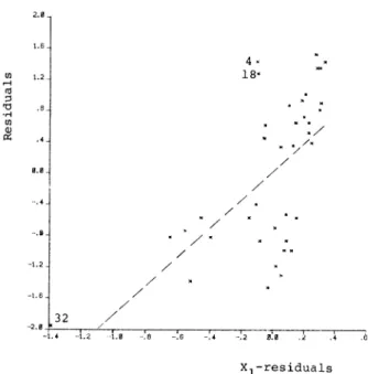
The data were analyzed by Finney (1947). Pregi- bon (1981) used them to illustrate the building blocks of logistic regression diagnostics. The response is either the occurrence or nonoccurrence of vasocon- striction. This response might depend on the rate (Xl) and volume (X2) of air inspired on a transient vasoconstriction in the skin of the digits. The plots in Figures 1 and 2, where the score statistics' values are 14.82 and 13.68, respectively, clearly indicate the sig- nificance of one variable after the other is included in the model. This suggests the importance of these two explanatory variables. Note that observations 4 and 18 in both plots seem to be the two most important observations that affect the slope of the regression through the origin, or the significance of the score statistic. In fact, when these two observations are de- leted, the MLE of /f changes from (-2.875, 5.719, 4.526) to (-24.58, 39.55, 31.94). Observation 32, TECHNOMETRICS, AUGUST 1985, VOL. 27, NO. 3
2.0 1.6 0) 1--i *H 5) .1 n ; 6.0 4 1 18' 1.2. .8 . .4. 0.0 -.4 -.8. -1.2- -1.6 / 4 5.0 H I, UA P; / / 7/ / / / 7 4.0 . 3.0 / / 2.0 . 1.0 -2.0 / 32 / -1.4 --.2 -[.0 -8 -'.6 .4 -.2 .0 .2 .4 . Xl-residuals
Figure 1. Added Variable Plot for Rate in Finney's (1947) Data. which stands out in Figure 1, also attracts our atten- tion, although it does not affect the regression much. Its strange Xl value can be detected after careful checks.
3.2 J0rgensen's Data
The data are taken from Jorgensen (1961). The response is the number of failures of a complex piece of electronic equipment in a week. Nine weeks in which each week was divided into two operating re- gimes were spent in observation. Explanatory vari- ables T1 and T2 are times spent in regimes one and
-H U1) fx 1.2 .8 . .4 . '-4 18
/.
/ ./ . / / / 7' '7 / / / '5 8 / -15. 0 -0.0 -5. 0 0.0 5.0 10.0 15.0 20.0 25.0 30.0 35.0 Tl-residualsFigure 3. Added Variable Plot for Time T1 in Jorgensen's (1961) Data.
two, respectively. For my illustration, treat these nine responses as independent Poisson observations with possible mean Tl,3 + T2 /2 . The importance of ex-
planatory variable T, after including T2 in the model is clearly shown in the plot of Figure 3 with score statistic 39.99. Moreover, the coefficient of T1 esti- mated by the plot is .159, not far from its MLE of .167. Unlike time TI, however, time T2 is not signifi- cant when time T1 is included. The added variable plot in Figure 4 indicates this with a value of 1.825 for the score statistic.
Observations 4, 5, and 8 seem to control two linear
'U En ,--I 10 .31 a) A? 0.0 2.5 . 2.0 - 1.5. .5 . -.8 - -1.2 - -1.6 . -.5 .6 -.4 -.2 00 .2 .4 .6 .8 1.0 1.2 1.4 2. -4. -.0 -6.0 3.0 0.0 3.0 6.0 9.0 12.0 15.0 18.0 X2-residuals Figure 2. Added Variable Plot for Volume in Finney's (1947) Data.
T2-residuals
Figure 4. Added Variable Plot for Time T2 in Jorgensen's (1961) Data.
TECHNOMETRICS, AUGUST 1985, VOL. 27, NO. 3
--~. ,-- , ' . a i I I I i I I I I I - L . 10 I I I I 1.G - / ? /
P. C. WANG trends on these two added variable plots. Both plots
suggest that the conclusion would be totally different without these three observations. Moreover, observa- tion 1 in Figure 4, which has the largest residual, suggests the decrease of the importance of variable T2 without it. These suggestions are confirmed by the score statistics without the corresponding observa- tions.
4. DISCUSSIONS AND CONCLUSIONS Pregibon (1981) gave excellent diagnostic pro- cedures in logistic regression, based on the model that includes all of the important explanatory vari- ables. In the preceding, I provide another approach to better understanding of the nature of the data under consideration. My procedures, both the score statistic and the corresponding added variable plot, check the importance of any explanatory variable and possibly influential or outlying observations for this variable. The score statistic indicates the signifi- cance of the slope of the regression line in the added variable plot and determines the importance of the underlying variable. The plot gives the overall im- pression of the scatter of the data points and detects observations that affect the importance of the vari- able. Such observations might be revealed when they are separated from the rest of the data. Thus I view these two procedures as complementary, and I rec- ommend the use of both.
Both the score statistic and the LRT statistic can be used for generalized linear models and be com- puted in the GLIM computer package. However, score statistics need fewer computations, since no iteration to obtain MLE's is needed under the alter- native. Although the score statistic I derived is a spe- cial case of Pregibon's (1982), we expect it to be more useful along with its corresponding added variable plot.
The slope of the regression line in an added vari- able plot can be used as an estimate of the coefficient of the variable considered. In normal linear regres- sion, this slope is exactly its MLE under the alter- native. However, this is not true in general. The MLE's in generalized linear models are usually ob- tained by an iterative method. Thus it is almost im-
possible to obtain such an estimate in any single step. The slope of the regression line in the plot might be a good starting estimate of the coefficient considered.
ACKNOWLEDGMENT
I thank the referees, the associate editor, and the editor for their helpful comments that led to im- provements in the presentation of this article.
[Received February 1984. Revised October 1984.] REFERENCES
Atkinson, A. C. (1982), "Regression Diagnostics, Transformations and Constructed Variables" (with discussion), Journal of the Royal Statistical Society, Ser. B, 44, 1-36.
(1983), "Diagnostics Regression Analysis and Shifted Power Transformations," Technometrics, 25, 23-34.
Belsley, D. A., Kuh, E., and Welsch, R. E. (1980), Regression Diag- nostics: Identifying Influential Data and Sources of Collinearity, New York: John Wiley.
Chen, C. (1983), "Score Tests for Regression Models," Journal of the American Statistical Association, 78, 158-161.
Cook, R. D., and Wang, P. C. (1983), "Diagnostics for Nonlinear Regression," unpublished manuscript.
Cook, R. D., and Weisberg, S. (1982), Residuals and Influence in Regression, London: Chapman and Hall.
(1983), "Diagnostics for Heteroscedasticity in Regression," Biometrika, 70, 1-10.
Cox, D. R., and Hinkley, D. V. (1974), Theoretical Statistics, London: Chapman and Hall.
Finney, D. J. (1947), "The Estimation From Individual Records of the Relationships Between Dose and Quantal Response," Bio- metrika, 34, 320-324.
Hocking, R. R. (1983), "Developments in Linear Regression Meth- odology: 1959-1982" (with discussion), Technometrics, 25, 219- 249.
Jorgensen, D. W. (1961), "Multiple Regression Analysis of a Pois- son Process," Journal of the American Statistical Association, 56, 235-245.
Landwehr, J. M., Pregibon, D., and Shoemaker, A. C. (1984) "Graphical Methods for Assessing Logistic Regression Models" (with discussion), Journal of the American Statistical Association, 79, 61-83.
McCullagh, P., and Nelder, J. A. (1983), Generalized Linear Models, London: Chapman and Hall.
Pregibon, D. (1981), "Logistic Regression Diagnostics," Annals of Statistics, 9, 705-724.
(1982), "Score Tests in GLIM With Applications," in GLIM.82: Proceedings of the International Conference on Gener- alized Linear Models (Ser. 14, "Lecture Notes in Statistics"), New York: Springer-Verlag.
TECHNOMETRICS, AUGUST 1985, VOL. 27, NO. 3 276