四通道即時EEG訊號獨立事件分析之FPGA實現

(1)

國立交通大學

電機與控制工程學系

碩

士論文

四通道即時

EEG 訊號獨立事件分析

之

FPGA 實現

FPGA Implementation of Four-Channel ICA for

On-line EEG Signal Separation

研究生：黃煒忠

指導教授：林進燈博士

(2)

四通道即時

EEG 訊號獨立事件分析之

FPGA 實現

FPGA Implementation of 4-Channel ICA for

On-line EEG Signal Separation

研究生：黃煒忠

Student：Wei-Chung Huang

指導教授：林進燈

Advisor : Dr. Chin-Teng Lin

國立交通大學

電機與控制工程學系

碩士論文

A Thesis

Submitted to Department of Electrical and Control Engineering College of Electrical Engineering

National Chiao Tung University in Partial Fulfillment of the Requirements

for the Degree of Master in

Electrical and Control Engineering July 2008

Hsinchu, Taiwan, Republic of China

(3)

四通道即時

EEG 訊號獨立事件分析之

FPGA 實現

學生：黃煒忠

指導教授：林進燈博士

國立交通大學電機與控制工程研究所

中文摘要

在真實世界的多感應器應用中，如何從混合訊號中分析出獨立訊號的瞎訊號分離是一個常見的問題，例如:音訊和生醫訊號處理。本論文提出一個基於資訊最大化之獨立事件分析方法應用於四通道 EEG 訊號分離。並用定點數實現於 FPGA,再藉由藍芽傳輸分離後的訊號。經由實驗的結果，本論文所提出的硬體方式比軟體運算快56 倍，且絕對相關係數和離線訊號處理比較至少有 80% 。最後，實際示範將用Altera DE2 發展板展示，此設計使用 16605 邏輯單元。而本論文所提出的四通道即時獨立事件分析系統也加入彈性的介面用於實際 EEG 訊號分離的應用。用資訊最大化演算法的即時生醫訊號分離其取樣頻率設定在64Hz，並藉由整合性的算術運算架構可讓整體操作速度在 68MHz。

(4)

FPGA Implementation of 4-Channel ICA for

On-line EEG Signal Separation

Student：Wei-Chung Huang Advisor : Dr. Chin-Teng Lin

Department of Electrical and Control Engineering

National Chiao Tung University

Abstract

Blind source separation of independent sources from their mixtures is a common problem for multi-sensor applications in real world, for example, speech or biomedical signal processing. This thesis presents an independent component analysis (ICA) method with information maximization (Infomax) update applied into 4-channel one-line EEG signal separation. This can be implemented on FPGA with a fixed-point number representation, and then the separated signals are transmitted via Bluetooth. As experimental results, the proposed design is faster 56 times than soft performance, and the correlation coefficients at least 80% with the absolute value are compared with off-line processing results. Finally, live demonstration is shown in the DE2 FPGA board, and the design is consisted of 16,605 logic elements.

The 4-channel On-line ICA accompanied with flexible communication interface for real EEG signal separation has been presented in this thesis. The proposed integrated mathematics architecture can allow high-speed at 68MHz and real-time biomedical signal separation with Infomax ICA at sampling rate 64 Hz.

(5)

誌謝

兩年的研究所生涯隨著論文的完成劃上了句號，這兩年間，要感謝許多人的鼓勵和幫忙，使我獲得充實的專業能力並順利完成研究所的學業。首先要感謝的是我的指導教授-林進燈老師。林老師是國內十分傑出的一位教授，在不同領域內都有相當好的研究成果。感謝老師提供了很理想的研究環境、豐富的資源及正確的引導，使我在研究上非常順利。在老師悉心的指導下，讓我學習到解決問題的能力及做研究應有的態度，使我獲益良多。在實驗室裡，鍾仁峰博士給予我最直接的教導，不管遇到課業上或研究上的問題，常常去請教鍾仁峰博士，感謝鍾學長不厭其煩地教導，使我增進了對積體電路設計上的專業知識，開拓了我的視野。在學校裡，感謝范倫達教授時常關心我學業上的研究，時常與我討論論文方向及進度。還要特別感謝洪紹航學長對於我研究上的指導，幫解決了我許多的問題。另外也感謝實驗室所有的夥伴，經翔、德瑋、俊傑、靜瑩及智文等學長姐們。還有我的同學們，毓廷、煒忠、建昇、孟修、寓鈞、舒愷、孟哲、俊彥、依伶。以及實驗室的學弟妹，昕展、哲睿、介恩、家欣、有德，感謝大家在研究上及生活上的互相扶持及鼓勵。最後要感謝家人爸爸、媽媽、妹妹的支持，讓我能專心於學術上的研究，渡過所有難關，謝謝！人生值得感謝的人其實很多，感謝老天、感謝許多親人、朋友和同學，在生命的旅途中，因為有你們，因為我們彼此珍惜、相互扶持，才能有無比的力量。

(6)

List of Figures

Fig. 2- 1 Illustration of the BSS problem...4

Fig. 2- 2 Illustration of ICA formulation ...5

Fig. 2- 3 Illustration of probability density distribution ...6

Fig. 2- 4 Entropy relationship by the concept of set ...7

Fig. 2- 5 Blind separation network architectures for two-source mixtures...9

Fig. 2- 6 Illustration of Off-line and on-line algorithm ...19

Fig. 2- 7 Diagram flow of the computation of implementation of on-line ICA learning algorithm...20

Fig. 3- 1 Illustrate of time process in on-line ICA...22

Fig. 3- 2 Matlab execution time...23

Fig. 3- 3 (a) original signal and p.d.f of original signal (b) mixed signal...25

Fig. 3- 4 Off-line EEGLAB toolbox ...26

Fig. 3- 5 Time-domain Comparison of on-line and off-line algorithm...26

Fig. 3- 6 Correlation coefficients Comparison of on-line and off-line algorithm...27

Fig. 3- 7 FFT comparison of on-line and off-line algorithm ...27

Fig. 3- 8 Time-Frequency Comparison of on-line and off-line algorithm...28

Fig. 3- 9 (a) original signal and p.d.f of original signal (b) mixed signal...29

Fig. 3- 14 Mixed EEG signal ...32

Fig. 3- 19 Mixed EEG signal2 ...34

Fig. 3- 23 Time-Frequency comparison of on-line and off-line algorithm...37

Fig. 4- 1 (a) Top level hardware architecture...38

Fig. 4- 2 ICA main system architecture ...39

Fig. 4- 3 Non-linear function ...40

(9)

Fig. 4- 5 Comparison of floating-point and fix point function ...42

Fig. 4- 6 Integrated computing unit ...43

Fig. 4- 7 Main Calculation Model architecture...44

Fig. 4- 8 Final Result architecture...45

Fig. 4- 9 Main controller architecture ...46

Fig. 4- 10 Asynchronous memory controller circuit...47

Fig. 4- 11 System controller circuit ...48

Fig. 4- 12 System pipeline flow...48

Fig. 4- 13 Illustration of micro-controller...49

Fig. 4- 14 Dynamic Branch Prediction ...50

Fig. 4- 15 Branch Controller and Flush Line...50

Fig. 4- 16 Illustration of RS232 Protocol...52

Fig. 4- 17 Receiver header controller architecture...53

Fig. 4- 18 Transmitter header controller architecture ...54

Fig. 4- 19 Illustration of Header Controller ...55

Fig. 4- 20 Detail of compilation report (a) summary (b) timing...56

Fig. 4- 21 post simulation of recursive operation circuit ...57

Fig. 4- 22 Time consumption of Weight calculation ...57

Fig. 4- 24 post simulation of system controller with no converge...58

Fig. 4- 25 post simulation of system controller with converge...59

Fig. 4- 27 post simulation of input interface...60

Fig. 4- 28 post simulation of output interface...60

Fig. 4- 30 post simulation of overall system...62

Fig. 4- 31 Illustration of demonstration ...62

Fig. 4- 32 Medi-Trace 200 ...63

Fig. 4- 33 Pin Configuration of AD7466 ...64

Fig. 4- 34 Interfacing to the MSP430F161 ...64

Fig. 4- 35 MSP430 Applications...65

Fig. 4- 36 four channels brain-computer interface...66

Fig. 4- 37 Pin Configuration of BM0203...68

Fig. 4- 38 EEG Graphical User Interface...69

Fig. 5- 1 left is pattern1 post simulation, and right is offline ICA result ...72

Fig. 5- 2 left is pattern2 post simulation, and right is offline ICA result ...72

Fig. 5- 3 left is EEG1 post simulation, and right is offline ICA result ...72

(10)

Fig. 5- 5 (a) mixed signal (b) ICA signal ...73

(11)

List of Tables

Table 2- 1 FastICA algorithm with deflationary orthogonalization...16

Table 2- 2 FastICA algorithm ...17

Table 3- 1 Matlab profile ...22

Table 4- 1 Description of the non-linear circuit...41

Table 4- 2 Description of recursive circuit...43

Table 4- 3 FSM of micro-controller...49

Table 4- 4 FSM of Header Controller ...55

Table 4- 5 low-cost transceiver microchips ...67

Table 4- 6 Detail pad description ...69

Table 4- 7 System specification ...70

(12)

Chapter1

Introduction

1-1 Motivation

In recent years, Independent Component Analysis (ICA) has been proved as a powerful algorithm to solve blind source separation (BSS) [1] problems in a variety of signal processing applications such as speech [2], image, or biomedical signal processing. Especially biomedical signals, which are different signal sources from organs such as brain, heart, or muscles, push the ICA algorithm to process more channels than speech or image applications. However, the characteristic of general ICA is limited to only process off-line and enormous data. On clinic, this cannot assist doctors in real-time diagnosis. Thus, more researches focus on on-line and faster ICA from points of view on software or hardware implementation.

The applications of ICA are separation of artifacts in Magnetoencephalography data, finding hidden factors in financial data, reducing noise in natural images, and telecommunications. Another, very different application of ICA is on feature extraction. A fundamental problem in digital signal processing is to find suitable representations for image, audio or other kind of data for tasks like compression and denoising. In On-line ICA application, it can detect the characteristic of biomedical signals immediately by On-line processing and send out the correct response to human. It is helpful to real-time biomedical monitor. Another application, it can used

(13)

for reduce dimension on high-channels data or extract noise in clamant environment. Since the large number of matrix operation and complicated non-linear computation are required, it is hard to real-time process in embedded systems. However, the FPGA implementation not only accelerate the speed of the operation circuit by parallel processing, but also show real-time computation and low-power property by fast symmetrical non-linear lookup table.

1-2 Goal and Summary

The Infomax ICA algorithm which is based on the concept of information maximization is designed to solve the problems of blind signal separation (BSS). There are two problems: The algorithm is not suitable for on-line computation, and complicated mathematics operation which make Infomax ICA hard to implement in VLSI. The algorithm has been improved by a new effective hardware and overlap memory scheduling to solve those problems. Finally, the thesis using pipeline flow to increase calculation throughput, and add dynamic branch predict to overlapping memory access time in pipeline.

1-3 Organization of the Thesis

This thesis is organized as follows. The Infomax theory and system level design are introduced in chapter 2 and chapter 3 individually. Chapter 4 describes FPGA implementation of ICA. The experimental results and discussions are presented in Chapter 5, and conclusions are made in the last chapter.

(14)

Chapter2

ICA Algorithm

2-1 Basic Concepts of ICA

ICA could be used in different fields, for example: image, audio signal processing, and biomedical data analysis. In this section, the basic concepts of ICA from the viewpoints of signal processing and statistics are introduced.

2-1-1

Problem Description

ICA is created to solve cocktail-party problems in signal processing. There are situations where there are a number of signals produced by some physical sources. These signals could be, for example, electric signals from different brain areas, speech signals from different people speaking in the same room [3], or radio waves from different mobile phones in the same area [4]. The sensors are placed in different positions, so that mixtures are different from one another as a result of space factors.

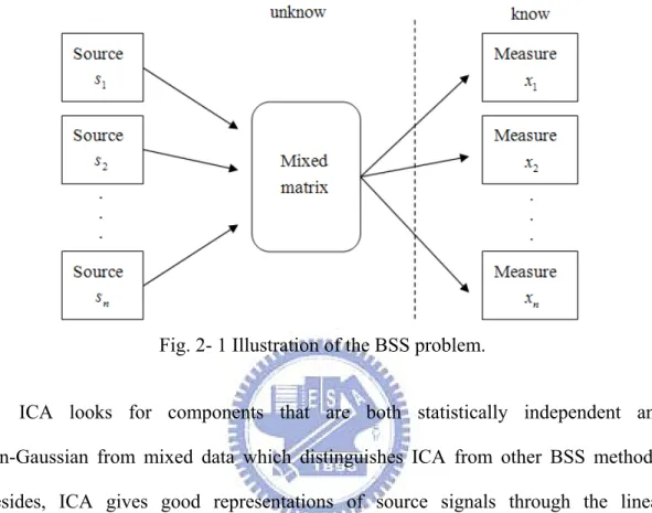
In practice, the information about the original signals and the mixing system are unknown, and the information of mixed signals from sensors. For this reason, drawing out original signals from those mixtures is professed Blind Source Separation. The BSS problem is illustrated in Fig. 2- 1. ICA is one of the useful methods to precede

(15)

BSS problems which separate signals mainly by independence. In the following contents, representations will be called components due to the name of ICA.

Fig. 2- 1 Illustration of the BSS problem.

ICA looks for components that are both statistically independent and non-Gaussian from mixed data which distinguishes ICA from other BSS methods. Besides, ICA gives good representations of source signals through the linear combination of mixed signals with non-linear decorrelation methods. In practical situations, it is easy to find the components which are really non-Gaussian.

On the other hand, the best de-mixing matrix that makes the components really independent to each other can not be found in general. It should be noted that algorithms exist to make the components as independent as possible.

2-1-2

Formulation

Most of the work on BSS so far addresses the case of mixtures, where a linear mixture model is assumed:

x(t)= A×s(t) (2.1)

(16)

observed vector of mixtures (ignoring noise). ICA now consists of estimating both the matrix A and s when x is the only given signal. It should be noted that the number of independent components s(t)_i equals to the number of observed variables

i

t

x( which is a simplifying assumption and is not completely necessary. ICA obtains ) a n×n matrix W where

⎥ ⎥ ⎥ ⎥ ⎦ ⎤ ⎢ ⎢ ⎢ ⎢ ⎣ ⎡ × = ⎥ ⎥ ⎥ ⎥ ⎦ ⎤ ⎢ ⎢ ⎢ ⎢ ⎣ ⎡ ≅ ⎥ ⎥ ⎥ ⎥ ⎦ ⎤ ⎢ ⎢ ⎢ ⎢ ⎣ ⎡ n n n x x x W y y y s s s M M M 2 1 2 1 2 1

(2.2)

Above the equation, s_i(t)≈ y_i(t)=W×x_i(t), y_i is called the representation of sources from the measurements. If is more similar to S, it is a better representation. Fig. 2- 2 shows the formulation of ICA.

Fig. 2- 2 Illustration of ICA formulation.

2-1-3

Independent Conditions

Sources are assumed to be statistically independent and non-Gaussian in ICA. The condition is a critical technique that makes ICA different from other methods.

According to the central limit theorem (CLT), sum of non-Gaussian random variables are closer to Gaussian than original ones. However, non-Gaussian assumption is also due to a natural disadvantage of ICA. In the statistical point of view, uncorrelated data are independent only when those data are Gaussian. Therefore, if the original independent components are Gaussian, their mixtures must be Gaussian. After mixtures are turned into uncorrelated by pre-processing, they are still Gaussian and already independent. However, those uncorrelated mixtures are always dissimilar

(17)

to the original independent components. There are two kinds of non-gaussian data: super-Gaussian and sub-Gaussian as illustrations in Fig. 2- 3.

Fig. 2- 3 Illustration of probability density distribution.

2-2 Two kinds of ICA Algorithm

We consider methods for estimating solution to the unknowns in ICA problem. In the simple case, we assume noiseless ICA x=As are the elements of the mixing matrix, A, and the sources s which we consider as being estimated by a recovered source set a.

2-2-1

The Concept of Entropy and

M

utual Information

The ICA algorithm assume all of the sources are independent in the module. The M sources together generate an M-dimensional probability density function (p.d.f) p(s). Statistical independence between the sources means that the joint source density factorizes as (2.3) p(s)=

∏

= M m m t s p 1 )) ( ( (2.3) If the p.d.f of the estimated sources also factorizes then the recovered sources are

(18)

independent and the separation has been successful. Independence between the recovered sources is measured by their mutual information, which is defined in terms of entropies.The entropy of an M-dimensional random variable x with p.d.f p(x) is

H[x]=H[p(x)]=−

∑

p(x)logp(x). (2.4) The entropy measures the average amount of information that observation of x yields. The joint entropy H[x,y] of two random variable x and y is defined as:

H[x,y]=H[p(x,y)]=−

∑

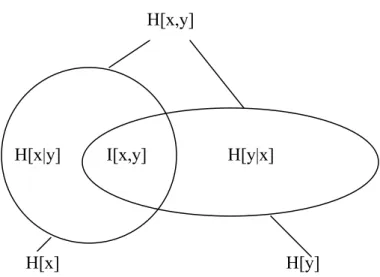
p(x,y)logp(x,y), (2.5) where p(x,y) is the Joint probability density of variable x and y. We can consider the entropy of x and y as a set. In Fig. 2- 4, joint entropy H[x,y] is continuum of H[x] and H[y], for H[x,y]≤H[x]+H[y], if x and y are independent, H[x,y]=H[x]+H[y].

Fig. 2- 4 Entropy relationship by the concept of set.

The conditional entropy of y given x is

H[y|x]=−

∑

p(y|x)logp(y|x). (2.6) Conditional entropy H[y|x] is entropy H[y] without H[x]. From which it follow that

H[x,y] = H[x]+ H[y|x]

= H[y]+ H[x|y]. (2.7) H[x,y]

H[x|y] H[y|x] I[x,y]

(19)

The above equation means that the sum of the information encoded by x alone and the information encoded by y given a knowledge of x. The entropy of each variable is related to probability of observations.

The mutual information between two random variables x and y is defined in terms of their entropies as follow (2.8):

I[x,y]=H[x]+H[y]-H[x,y] =H[x]-H[x|y]

=H[y]-H[y|x]. (2.8) From the equation above, the mutual information contains the sum of the entropy of each variables and the difference of the joint entropy of all variables.

Using concept of mutual information, an m-dimensional random variabley , _i

i=1…n, the mutual information of all variable is defined as:

∑

= − = n i i n H y H y y y y I 1 2 1, ,..., ) ( ) ( ) ( . (2.9) Where H is entropy, H(y) is the joint entropy H(y₁_,y₂_,...,y_n)of variabley , the _i

value of mutual information always positive or zero. If and only if the value is zero, each variable is independent. If the target is finding the minimum mutual information between each variable, it is equal to find the direction of non-Gaussian distribution. Next section, we will describe two methods of ICA: Information maximization ICA and FastICA.

2-2-2

Infomax ICA

(1)

Information maximization

Bell and Sejnowski [5] proposed to learn the separating matrix W by minimizing the mutual information between components of y(t) = g(u(t)) , where g is a nonlinear function approximating the cumulative density function (cdf) of the sources. Bell &

(20)

Sejnowski formulated blind source separation algorithms in terms of information maximization.

Consider the information transmitted by mapping f: x→y. K.Torkkola [6] consider the two-stage mapping, which might be implemented by a single layer feed-forward neural network in Fig. 2- 5, as follows:

u=W*x, (2.10) y=g(u), (2.11)

Fig. 2- 5 Blind separation network architectures for two-source mixtures.

where W is a linear transformation and g is a bounded nonlinearity applied to each individual output u. The information transmitted by the mapping is the mutual information between the input and output:

I[x,y]=H[x]+H[y]-H[x,y]

=H[y]-H[y|x], (2.12) where H[y] is the entropy of the output, while H[y|x] is whatever entropy the output has which didn’t come from the input. In the case that we have no noise, the mapping between x and y is deterministic and H[y|x] has its lowest possible value. This

X1

X2

W12

W21

W22

W11

g

y1

y2

∑

G

(21)

divergence is one of the consequences of the generalization of information theory to continuous variables. In order to reduce complexities, the algorithm consider only the gradient of information theoretic quantities with respect to some parameter, w, in the network.

Since gradients are as well behaved as discrete variable entropies, the reference terms involved in the definition of differential entropies disappear. The above equation can be differentiated as follows, with respect to a parameter, w, involved in the mapping from x to y:

( , ) H(y) w y x I w ∂ ∂ = ∂ ∂ , (2.13) H[y|x] does not depend on w, and lead ( | )=0

∂ ∂

x y H

w . Thus for invertible

continuous deterministic mappings, the mutual information between inputs and outputs can be maximized by maximizing the entropy of the outputs alone.

When a single input x pass through a transforming function g(x) to give an output variable y, both I(y| x) and H(y) are maximized when we align high density parts of the probability density function of x with highly sloping parts of the function g(x). This is the idea of “matching a neuron’s input-output function to the expected distribution of signals”.

From another point of view, thus

∑

= − = n i i n H y H y y y y I 1 2 1, ,..., ) ( ) ( ) ( , to

minimize mutual information to each outputs y_i existence when )

,... (

)

(y H y₁_,y₂ y_n

H = , and I(y₁,y₂,...,y_n)=0. Output y is independent. In order _i

to let mutual information of outputs be zero, need to satisfy below situation: 1. The choice of non-linear function g(.) is crucial.

_u e u g y ₋ + = = 1 1 ) ( u=Wx. (2.14) 2. According to maximum entropy theorem, if bounded variable with

(22)

uniform distribution has the maximum entropy. y must between 0~1 _i

because of it is the p.d.f of independent component u . Therefore in _i

order to maximize the entropy of output, we need output y uniform distribution

The output y have to independent to satisfy both of situation. Although the transformation between y and u is a monotonic transform, information maximization using this concept to achieve the target of ICA.

(2)

Gradient information

Consider a network with an input vector x, a weight matrix W, a bias vectorw and a nonlinearly transformed output vector y=g(u), u= Wx+₀ w . ₀

Providing W is a square matrix and g is an invertible function, the multivariate probability density function of y can be written

| | ) ( ) ( J x P y P = , (2.15) where |J| is the absolute value of the Jacobian of the transformation. Bell simplifies to the product of the determinant of the weight matrix and the

derivative '

i

y , of the outputs, y , with respect to their net inputs: _i

∏

= = n i i y W J 1 ' ) (det . (2.16) For example, in the case where the nonlinearity is the logistic sigmoid:

_u e u g y ₋ + = = 1 1 ) ( and ' _y(1 _y) u y y = − ∂ ∂ = . (2.17) We can perform gradient ascent in the information that the outputs transmit about inputs by noting that the information gradient is the same as the entropy gradient for invertible deterministic mappings. The joint entropy of the outputs is:

(23)

Weights can be adjusted to maximize H(y). As before, they only affect the E[ln |J|] term above:

∏

= ∂ ∂ + ∂ ∂ = ∂ ∂ = ∂ ∂ Δ n i i y W W W J W W y H W 1 ' _| | ln | det | ln | | ln ) ( α . (2.19)

For the full weight matrix, we use the definition of the inverse of a matrix, and the fact that the adjoint matrix, adj W, is the transpose of the matrix of cofactors. This gives:

_ln_|_det _|₌_[ _]−1

∂

∂ _W _WT

W . (2.20)

For the second term, we note that the product splits up into a sum of log-terms, only one of which depends on a particular w.

n T i n i n i i y x x y W x y x y W y W ln | | ln | | 1 ( ) ( ) (1 2 ) 1 1 1 ' ₌ ₋ ∂ ∂ ∂ ∂ ∂ ∂ = ∂ ∂ ∂ ∂ = ∂ ∂

∏

= − = = . (2.22) The resulting learning rules are familiar in form:

_Δ_W _∝_[_WT_]−1₊₍₁₋₂_y₎_xT_{. (2.23)}

Except that now x, y, W, and1, are vectors (1 is a vector of ones). But this learning rule is too complex to calculate because of the inverter matrix. Multiplied by WTW _{change the rescale of the rule, the new learning rules as follow:}

_ΔW ₌₍I₊₍₁₋₂y₎uT₎W ₌₍I₊_ϕ₍u₎uT₎W_{. (2.24)}

Thus, the simplification much uncomplicated than before, and this learning rules is suitable to separate blind sources. An ICA model consists of two distinct components, the first is the formulation of a valid contrast function and second is the algorithm for estimating the free parameters of the system.

Considering approaches which rely on the gradient of the contrast to ascend or descend to an extreme contrast measure. It is computationally attractive to have access, to the analytic form for the gradient of the contract function with respect to the free parameters. The bias of the contrast function to be that of a generative model approach, Gradient-ascent, or steepest-gradient, methods require this first order

(24)

information and update W in direction of the gradient. The update rule for W in discrete time t<-t+1 defined in equation as follows:

W(t+1)=W(t)+lΔW. (2.25) where lis the adaptation parameter (learning rate) which is fixed this procedure corresponds to maximum likelihood re-estimation with an exponential weighting over successive samples. Note that this learning rule describes an online learning procedure because data are processed sequentially as they are received. Gradient ascent to the likelihood for a batch of T observation is performed with the modified rule

( 1) ( ) ( 1 ( ) ( )) 1

∑

= + + = + T t T _t u t T I l t W t W ϕ . (2.26) Since the learning rule (2.26) is obtained from (2.25) by dropping the averaging operation it is sometimes called stochastic gradient ascent. The use of steepest-gradient techniques to ascend the likelihood to near its supremum was formulated by Bell & Sejnowski [1995]. One of the key problems is their poor convergence in region of shallow gradient and in regions where the likelihood landscape is far from isotropic. To overcome some of these issues, Bell & Sejnowski utilized batching, whereby the mean gradient over a set of consecutive samples is utilized rather than the sample by sample estimate.

2-2-3

FAST ICA

After we have defined a measure of non-gaussian, we have to develop a practical method for maximizing it. The basic method used in this kind of problems is the gradient method. However, FastICA is based on a fixed-point iteration scheme for finding a maximum of the non-gaussian of WTx_{. More rigorously, it can be derived}

as an approximative Newton iteration. The FastICA algorithm using negentropy combines the superior algorithmic properties resulting from the fixed-point iteration with preferable statistical properties due to negentropy.

(25)

(1)

Fixed-point algorithm

In this subsection, we will introduce Fixed-point algorithm. Fixed-point iteration would be equate W to the gradient measure of non-gaussian. This is because if W equals this gradient, then due to normalization to unit norm. This suggests the following fixed-point iteration:

W _<₋_ε[xg(WTx)]_{. (2.27)} The iteration does not have good convergence properties. Therefore, the iteration has to be modified. Multiplied by constant α and add W on both side of this equation as below:

₍₁₊_α₎W ₌_ε_[xg₍WTx_)]₊_αW_{. (2.28)}

Thus, by choosing α wisely, it may possible to obtain an algorithm that convergence very fast.

The suitable coefficientα , and thus the FastICA algorithm, can be found using an approximative Newton method [7]. The Newton method is a powerful method for solving equations. When it is applied to the gradient, it gives optimization method that usually converges in a small number of steps. The problem with the Newton method is that it usually requires a matrix inversion at every step. Therefore, the total computational load may not be smaller than with gradient methods. This approximative Newton method gives a fixed-point algorithm of the form.

To derive the approximative Newton method, first note that the maxima of the approximative of the negentropy of WTx _{are obtained at certain optima of}

)] ( [G WTx

ε . According to Kuhn-Tucker conditions, the optima of _ε[G(WTx)]_under the constraint _ε[(_WT_x)2]_{= W} 2 ₌1_{are obtained at points where}

(26)

_ε[g(WTx)]+ W_β =0_{, (2.29)} where β is some constant. Denoting the function on the left-hand side by F, we obtain its Jacobian matrix JF(w) as

JF₍W₎₌_ε_[xxTg'₍WTx_)]₊_βI _{. (2.30)}

To simplify the inversion of this matrix, we decide to approximate the first term. Since the data is sphered, a reasonable approximation seem to be

_ε_[xxTg'₍WTx_)]_≈_ε_[xxT_]_ε_[g'₍WTx_)]₌_ε_[g'₍WTx_)]I_{. (2.31)}

Thus the Jacobian matrix becomes diagonal, and can easily be inverted. Thus, obtain approximative Newton iteration:

= −ε +β _ε ₊_β )] ( [ )] ( [ ' _W _x g W x W xg W W T T . (2.32) This algorithm can be further simplified by multiplying both sides by

β

ε +

= [ ( )] )

(_W _g' _W _x

JF T _{. After straightforward algebraic simplification}

_W _<₋_ε[_xg(_WT_x)₋_ε[_g'(_WT_x)]_W]_{. (2.33)} This is the basic fixed-point iteration in FastICA.

(2)

Estimating several Independent Components

The key point to estimate more than one independent component is based on the following property: the vectors W corresponding to different independent _i

components are orthogonal in whitened space. Thus, to estimate several independent components, we need to run any of the above one unit algorithm using several units with weight vectors, and to prevent different vectors from converging to the same maxima we must orthogonalize the vectors after every iteration. We present in the following different methods for achieving decorrelation.

A simple way of orthogonalization is deflationary orthogonalization using the Gram-Schmidt method. This means that we estimation the independent components

(27)

one by one. When we have estimated p independent components, we run any one unit algorithm for W_p₊₁ , and after every iteration step subtract from W_p₊₁ the ‘projections’ WTW_j W_j j p

p ) , 1,...

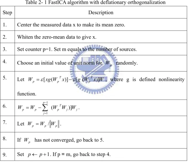
( = , of the previously estimated p vectors, and then renormalize W_p₊₁ . The result FastICA algorithm [8] with deflationary orthogonalization is show in Table 2- 1.

Table 2- 1 FastICA algorithm with deflationary orthogonalization

Step Description 1. Center the measured data x to make its mean zero.

2. Whiten the zero-mean data to give x.

3. Set counter p=1. Set m equals to the number of sources. 4. _{Choose an initial value of unit norm for}

p W randomly. 5. _Let _W _xg _W _x _g _W T_x _W p T p

p =ε[ ( )]−ε[ '( )] , where g is defined nonlinearity

function. 6. j j T p p j p p W W W W W ( )] 1 1

∑

− = − = . 7. _Let p p p W W W = / . 8. _If p

W has not converged, go back to 5.

9. Set p← p+1. If p = m, go back to step 4.

In certain application, it may be desirable to use a symmetric decorrelation, in which no vectors are ‘privileged’ over others. This means that the vectors W are not _i

estimated one by one, instead, they are estimated in parallel. One motivation for this is that the deflationary method has the drawback that estimation errors in the first

(28)

vectors are accumulated in the subsequent ones by the orthogonalization. This is done by first doing the iteration step of one unit algorithm on every vector W , and _i

afterwards orthogonalization all the W by special symmetric methods. _i

The symmetric orthogonalization of W can be accomplished by the classical method involving matrix square roots,

W ₌₍WWT₎−1/2W_(2.34)

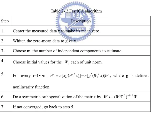
The inverse square root is obtain the eigenvalue decomposition, T m T _Ediag _d _d _E WW ) ( ,... ) ( 1/2 1/2 1 2 1 ₋ ₋ − = (2.34) Using the former symmetric orthogonalization, we give the correspond version of the FastICA algorithm in Table 2- 2.

Table 2- 2 FastICA algorithm

Step Description 1. Center the measured data x to make its mean zero.

2. Whiten the zero-mean data to give x.

3. Choose m, the number of independent components to estimate. 4. _{Choose initial values for the}

i

W each of unit norm.

5. _{For every i=1…m,} _W _xg _W _x _g _WT_x _W i T

i

i =ε[ ( )]−ε[ '( )] , where g is defined

nonlinearity function

6. Do a symmetric orthogonalization of the matrix by W _←₍WWT₎−1/2W

(29)

2-3

Main Structure of ICA Methods

Base on the algorithm of off-line ICA flow, in order to achieve real-time calculation, we divide the input of mixed sources to process real-time signals individually, and overlap the previous mixed sources to calculate new separated signals.

2-3-1

The Choice of ICA Algorithm

We consider two reasons feasibility and complexity of real time to realize on-line ICA from two algorithms above. In order to reach real time, we need to choose a low complicated computation and suitable property for the separation of super Gaussian signals. The reason for why we choose infomax ICA is that the flexible transmission and unnecessary preprocessing, it can reduce complicated calculation when real-time. Though the infomax ICA constringency is harder than FastICA, we add a decrease parameter with growing data to accelerate the convergence. In next section, we will propose a solution to fix the order of weight in real time processing.

2-3-2

Solution of on-line ICA

Since the original blind source separation algorithm by Jutten and Herault [9], several on-line and batch mode algorithms have been formulated under the umbrella of independent component analysis. While some of the batch ICA algorithms such as JADE [10] and FastICA [11] give relatively fast convergence in estimating W, they are not quite suitable for on-line implementation in a real-time setting. Depend on Gradient information learning rules, the weight need update at each new division. In order to fix the direction of weight are the same in every division, overlapping previous mixed sources will fix the order of the weight. The method of data-stream processing illustrate in Fig. 2- 6.

(30)

Fig. 2- 6 Illustration of off-line and on-line algorithm.

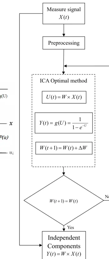
Fig. 2- 7 show the ICA MODEL, X(t) are measure data. After preprocessing, the model will enter the main calculation unit, including non-linear transformation, and gradient information update. However, in on-line processing of data stream, each division data stream will flow through the ICA model, then, each time the weight be calculated for each division data. Briefly, we take eight seconds division data to processing, and updating two seconds because of the overlap are six seconds. Finally, if the weight is stable, Y(t) represent the independent components which is the product of input X(t) and weight matrix.

(31)

Fig. 2- 7 Diagram flow of the computation of implementation of on-line ICA learning algorithm. Measure signal ) (t X Preprocessing W t W t W( +1)= ( )+Δ ICA Optimal method

) ( ) (t W X t U = × U e U g t Y ₋ − = = 1 1 ) ( ) ( ) ( ) 1 (t W t W + =

Independent

Components

) ( ) (t W X t Y = ×

ICA MODEL:

Yes No

(32)

Chapter3

System Architecture Design and

Simulation Result

3-1

System Architecture

In this chapter, we will discuss the execution flow of real time algorithm in software. With the system level simulation [12] and data stream flow, we can set specifications of overall system architecture, e.g. the resolution of input, the core speed, and the flexible interface.

3-1-1

Computing Flow

Before setting specifications, we need to analyze the process of data stream in system. First, set the sample rate for 64Hz. In the system of algorithm, we put 512 points data into ICA model with growing data. The 128 points are the set of result because of the old data overlap. Illustrate the system level process with Fig. 3- 1.

However, we discuss the algorithm for on-line execution in MATLAB. In software simulation, we measure the weight update and memory access time by profile command that records information about once recursive time. Table 3- 1 shows the detail of measurement. Total recorded time means the average execution time in ones iteration. And Fig. 3- 2 show execution time with some test data and average execution time at last. The iteration includes two parts: weight update calculation and

(33)

memory access. We can find that 86 percent of the total time is Weight update calculation.

Fig. 3- 1 Illustrate of time process in on-line ICA.

Table 3- 1 Matlab profile

Total recorded time 8.30956 ms Clock precision 0.00000006 s Clock Speed 1650 MHz 2S 8S 2S

M

512 points 512 points 512 points 512 points 512 points 512 points 128 points T ICA MODEL ICA MODEL ICA MODEL ICA MODEL ICA MODEL ICA MODEL 128 points 128 points 128 points 128 points 128 points

M

6S

(34)

Matlab execution time 0 2 4 6 8 10

DATA1 DATA2 DATA3 DATA4 DATA5 Average

ms

Weight update Memory access

Fig. 3- 2 Matlab execution time.

On the other hand, if the sample rate is 64Hz and the training needs 10 times, we can not finish the training in 16ms. As a result, the software execution time is not fast enough to achieve on-line processing. So we develop a suitable hardware for on-line ICA by FPGA.

3-1-2

Specification of On-line Process

In this system scheme, we need to formulate three parts: the resolution of the input signal, expected core speed, and the core speed. As a result of the quantity of four channels transmission and the restrictions of bus, the resolution of the input signal set as 8 bit. Since the memory bandwidths are 32 bits, it will read four channel data at the same time and it is efficient for memory controller design. While in the data stream, ICA model will process eight seconds data, it means if the sample rate is 64 Hz, the model can process 512 points once, and next iteration, the new two second data combines with old six second data into the ICA model. In order to achieve real-time execution, the ICA model should finish the eight seconds data iteration before the next point into memory. Since it can be derived the required speed of overall system. We set the sample rate is 64 Hz because the frequency of the signal

(35)

which we analyze less than 32Hz. Most of the cerebral signal observed in the scalp EEG falls in the range of 1-20 Hz. So the required speed of overall system derived as follow: ) _ _ ( _ _

_speed sample rate train loop w calculate converge decision

core = × × + (3.1)

In equation (3.1), train _loop represent the maximum number of times of weight update. If the number of times of weight update greater than maximum value, the iteration would stop training. The w _calculate represent the consumption of clock cycles in one iteration. And the coverage _decision represent the number of clock cycles which calculate the difference between new weight and old weight for the decision of weight coverage. In the situation we defined, the core speed should be at least 68MHz for on-line execution.

3-2

Comparison with off-line Sup-Gaussian BSS Methods

This section introduces the on-line system simulation of Independent Component Analysis. In order to verify the algorithm is suit to on-line process, we will use MATLAB to simulate the accuracy of on-line ICA behavior, and, define the specification and resolution of real circuit architecture. Then implement the arithmetic operation circuit and memory control circuit by the real-time processing simulation.

3-2-1

Simulation 8-bit Super Gaussian Mixed Pattern 1

In verification of MATLB, we create four original signals which p.d.f histogram are super Gaussian with 8 bit resolution and 64Hz sample rate. In real case, we mixed these four signals with a linear mixed matrix, and, thus the mixed four signals are the inputs of real-time ICA model in Fig. 3- 3.

(36)

(a)

(b)

Fig. 3- 3 (a) original signal and p.d.f of original signal (b) mixed signal.

(1)

Time-domain Comparison

In order to verify the algorithm, we compare with the EEGLAB which developed by UCSD in Fig. 3- 4. EEGLAB is an interactive Matlab toolbox for processing continuous and event-related EEG, MEG and other electrophysiological data using independent component analysis (ICA). EEGLAB provides an interactive graphic user interface (GUI) allowing users to flexibly and interactively process their high-density EEG and other dynamic brain data using independent component analysis (ICA) and/or time/frequency analysis (TFA), as well as standard averaging

(37)

methods. The algorithm of EEGLAB is suit to off-line process, but we just compare time domain and frequency domain result.

Fig. 3- 4 Off-line EEGLAB toolbox.

Fig. 3- 5 Time-domain Comparison of on-line and off-line algorithm.

See above Fig. 3- 5, although the order of each result may different, and the amplitude may reverse, but the characteristic of output are the same. The result accords with restriction of the ICA algorithm.

(2)

Correlation coefficients Comparison

(38)

Fig. 3- 6, it means the relation between each output signal. The negative value means each output of the first channel are reverse, and the value approach one means that these two signals are equivalent.

Fig. 3- 6 Correlation coefficients Comparison of on-line and off-line algorithm.

(3)

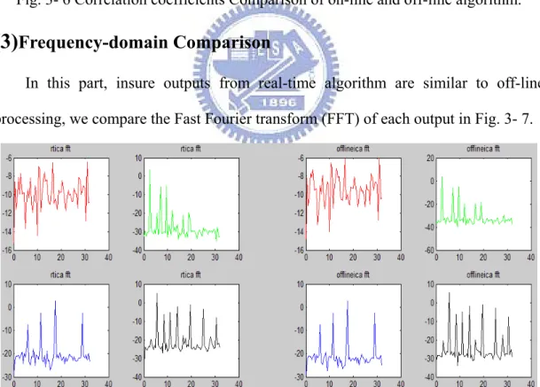
Frequency-domain Comparison

In this part, insure outputs from real-time algorithm are similar to off-line processing, we compare the Fast Fourier transform (FFT) of each output in Fig. 3- 7.

Fig. 3- 7 FFT comparison of on-line and off-line algorithm.

(4)

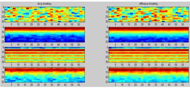
Time-Frequency Comparison

(39)

algorithm. Time-frequency: frequency power spectral density estimate on a single channel. The horizontal axis is time domain and vertical axis is frequency domain. The colors represent the power spectral.

Fig. 3- 8 Time-Frequency Comparison of on-line and off-line algorithm.

3-2-2

Simulation 8-bit Super Gaussian Mixed Pattern 2

The same as section 3-2-1, this section compare with another super Gaussian which has the same frequency like EEG about at 5Hz , 12Hz in Fig. 3- 9. We also compare with off-line tool box contains time-domain, frequency-domain, time-frequency, and correlation coefficients.

(40)

(b)

Fig. 3- 9 (a) original signal and p.d.f of original signal (b) mixed signal.

(1)

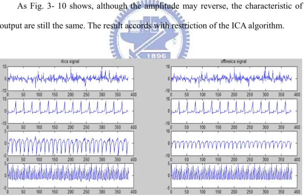
Time-domain Comparison

As Fig. 3- 10 shows, although the amplitude may reverse, the characteristic of output are still the same. The result accords with restriction of the ICA algorithm.

(2)

Correlation coefficients Comparison

Though the kurtosis of original signal are large than three, it can be regarded as pure super Gaussian. The result of correlation coefficients between off-line and

(41)

real-time algorithm are high in Fig. 3- 11. Software simulation has reached the target.

(3)

Frequency-domain Comparison

We create four signals that two of them were 5 Hz, 12Hz like EEG frequency as Fig. 3- 12 shown. Alpha is the frequency range from 8 Hz to 12 Hz. It is brought out by closing the eyes and by relaxation. Theta is the frequency range from 4 Hz to 7 Hz. Theta is seen normally in young children. It may be seen in drowsiness or arousal in older children and adults. From the result of third and fourth channel, there have significant power at 5 Hz, 12Hz indeed.

(42)

(4)

Time-Frequency Comparison

Fig. 3- 13 shows the time-frequency between off-line and real-time algorithm. The same, second and fourth channel in time-frequency there have significant power with red color.

3-3 Comparison with off-line EEG BSS Methods

The real EEG signals are given by NCTU BRC, which are recorded in real environment. The row data type with 8 bit resolution and 64Hz sample rate.

3-3-1

Simulation 8-bit EEG Mixed Pattern 1

In real environment, we can create pure EEG signals, and can not mix them as a mixed signal like Fig. 3- 14. We can analyze the measured signal as mixed signals directly.

(43)

Fig. 3- 14 Mixed EEG signal.

(1)

Time-domain Comparison

In real environment, EEG signals may have EOG, Alpha, Beta, Theta etc. In order to analyze pure signal, we need to separate each signal by ICA algorithm. Fig. 3- 15 shows the compare of off-line and real-time algorithm.

(2)

Correlation coefficients Comparison

The Correlation coefficients of EEG signals show below, it shows the highest Correlation coefficient is up to 99% compare with off-line algorithm. But in real

(44)

environment with unknown noises may cause reduction of Correlation coefficients. According to the result of Correlation coefficient in Fig. 3- 16, the correlation at least 80% compare with off-line is a good method for real-time.

(3)

Frequency-domain Comparison

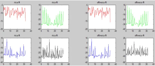
In this part, we compare the Fast Fourier transform (FFT) of each output. Apparently the second and fourth channel of each algorithm with a little different in Fig. 3- 17, and the frequency aliasing is caused by the less information with real-time process.

(45)

(4)

Time-Frequency Comparison

See Fig. 3- 18, the time-frequency show the frequency power spectral with little difference at second and fourth channel. However, we can find from Fig. 3- 18, the third channel with a significant power spectral at 10Hz.

3-3-2

Simulation 8-bit EEG Mixed Pattern 2

The second pattern shows in Fig. 3- 19. The characteristic of pattern output are like each other. This is because the sensors are located closely, the signals we measure will be very much like.

(46)

(1)

Time-domain Comparison

The same as section 3-3-1, this section discuss the different between on-line and off-line in real environment. The result of ICA with more noise than before, because the sensors are located closely in Fig. 3- 20.

(2)

Correlation coefficients Comparison

The correlation coefficients of second pattern are lower than before in Fig. 3- 21, but at least 80% in absolute value is also an acceptable method for real-time.

(47)

(3)

Frequency-domain Comparison

Fig. 3- 22 shows the FFT result comparison. We can see the result of the fourth channel with more error than others. But there is still more than 80 percent of the correlation.

Fig. 3- 22 FFT comparison of on-line and off-line algorithm.

(4)

Frequency-domain Comparison

Fig. 3- 23 shows that the first and second channel has more information at 10 Hz than third and fourth channel. Besides, Alpha is the frequency range from 8 Hz to 12 Hz. This is activity in the 8-12 Hz range seen in the posterior regions of the head on both sides, being higher in amplitude on the dominant side. It is brought out by closing the eyes and by relaxation. As a result, it is more helpful to analyze the measured signal than without ICA process.

(48)

Fig. 3- 23 Time-Frequency comparison of on-line and off-line algorithm.

3-4

Summery of Comparison

The simulation results from the above we can know that the amplitude of signal may be reverse or different in the ICA algorithm. These problems conform to the constraints referred in Chapter II. However, in real-time and off-line comparison, we can find the analysis result is better if the original signals are pure super Gaussian distribution. In real environment, the EEG measurement will contain many unknown noise or non-super Gaussian signal, and makes the effect drop in EEG analysis. In the comparison between on-line and off-line, because the on-line process collect small amount of information than off-line process, the correlation of on-line system might be different from off-line. But we can accept such a result that correlations are at least more than 80%.

(49)

Chapter4

Implementation of the On-line ICA

System on FPGA

Top level real-time hardware architecture shown in Fig. 4- 1.

(a)

(b)

Fig. 4- 1 (a) Top level hardware architecture (b) Illustration of real-time systems.

4-1 Architecture of real-time Systems

In this section we discuss the architecture of the digital circuit of implementation

mem

ICA module

64Hz

_64Hz

68MHz

mem & sys control

Real time ICA

(50)

of the algorithm. In overall system, the main architecture required three parts in Fig. 4- 2: Infomax operation circuit, memory control circuit, and interface control circuit. Arithmetic operation circuit consists of matrix operation circuit and non linear transform. Though a large number of computation in ICA arithmetic operation circuit, the memory access will be frequently and complex. By using efficient memory controller to optimize the memory scheduling and reduce the circuit power consumption. The concept of the non linear transform, it is hard to execute for real-time cause of the DSP processor will approximate the value by loop iteration. If we implement by FPGA, it will be developed with very low cost hardware, and reduce unnecessary operation, and fast enough to execute for real-time.

Fig. 4- 2 ICA main system architecture.

4-1-1

Implementation of Recursive Operation Circuit

The stability and high-precision are the properties of the recursive operation circuit. The errors may grow up with the growing iteration. In order to reduce errors in iteration, we develop a precision symmetrical non-linear piecewise look up table. Besides, we simplify the complex weight updating by deep pipeline design. And if the

(51)

final weight coverage, the effective and fast matrix multiplier would be also designed in the system. We will discuss these three parts as follows:

(1)

Precision symmetrical non-linear piecewise look up table

Considerations in design of non-linear look up table. We will focus on accuracy, hardware area, and computing time. On the accuracy, sign-bit fix point and symmetrical look-up table will be used by the property of non-linear symmetry and the simulation results of the algorithm [13]. It can reduce half areas by using symmetrical look-up table. For accuracy, in order to reduce errors, it will be 11 bits resolution for the symmetrical look-up table. However, the error estimates about

error =ε×i, (4.1) whereε represent the resolution error of look-up table, and i represent the number of the system iteration. Then error is the approximation of maximum error. As a result, the error will increase each iteration.

_u e u g y ₋ + = = 1 1 ) ( . (4.2)

(52)

Table 4- 1 Description of the non-linear circuit Name Description In[22:0] u =w×x Out[10:0] u e− + 1 1

Fig. 4- 3 and Fig. 4- 4 show the non-linear function and circuit block diagram. The operation can use symmetry due to non-linear function is singular function. Symmetry in block diagram is the judgement of whether input is less than zero or not. If input less than zero, it will use the same table to operate. As a result, it can save half area or double precision with the same table. Table 4- 1 shows the description of the non-linear look-up table.

Fig. 4- 4 Precision Symmetrical Non-linear Piecewise Look up Table.

The error tolerance in block diagram is the need to verify. In MATLAB, all equation calculated by floating point. So we compare difference between fix point and floating-point. The root mean square error (RMSE) is 0.00029956

Index IN Integer Decimal OUT Symmetry

M

Decimal

(53)

Fig. 4- 5 Comparison of floating-point and fix point function.

Left Fig. 4- 5 shows nonlinear function do precision computing by floating-point, and right show the look up table result. It can be seen slight error, but has been reached the real time implementation by increasing in non-linear processing.

(2)

Weight Recursive operation

In this section, we integrate the weight update of infomax in a module. The module is the mathematical core of overall system. The processing speed decides whether to real time. So in this complex computing module, in order to increase the core speed and throughput, we use the method of deep pipeline. Although the integrated computing module will increase some areas, it is suitable for memory controller design. With less memory access times, we can save more power consumption. Besides, we can use more than one integrated computing unit to improve system efficiency. We will focus on the design of integrated computing module. The mathematics expressions as follow:

W u u I W u y I W ₌₍ ₊₍₁₋₂ ₎ T₎ ₌₍ ₊_ϕ₍ ₎ T₎ Δ , (4.3) W(t+1)=W(t)+lΔW . (4.4)

(54)

Table 4- 2 Description of recursive circuit

Name Description Weight[15:0] Initial weight or previous weight

data[10:0] Sample data from ADC bias For infomax non-linear

lrate Initial learning rate is ₀_.₀₀₃₉_≈₂−8_, _lrate_{∝ t}−1

New weight[15:0] Gradient information update New bias Gradient information compensation

In hardware, however, fixed-point numeric is more practical. Although several groups have implemented floating-point adders and multipliers using FPGA, very few practical systems exist. The main disadvantages using floating-point in hardware are high resource requirements and high clock frequency. We use 16-bit fixed-point numeric, and the rough precision of the fixed point number representation can reach 0.000030518. Two bits for integer part, and 14 bits for the fractional part. When performing Infomax operations, normalization was performed to avoid overflow and make sure that the data path was always best utilized. The detail description is in Table 4- 2.

(55)

Fig. 4- 6 shows the integrated computing unit, it can process 4*512 matrix operation. The unit includes three 4*4 matrix operation, one accumulation, and mathematics operator. All speed must be greater than 68MHz to achieve real time execution. Then we design the calculation module with pipeline. In order to on-line execution, we estimate the consumption of cycle must less than 8300 cycles when core speed is 68MHz and 128 times training. As a result, the unit consumes 8192 cycles to find a new weight with gradient information update. The expressions as follow

iteration

rate

sample

speed

core

cycle

operation

*

_

=

. (4.5)

Fig. 4- 7 Main Calculation Model architecture.

Gradient

Information

Update

ICA Control Signal

ICA

Memory

Controller

Weight

Buffer

16 16×

Weight

Converge

Decision

ICA_DONE

(56)

Fig. 4- 7 shows the hierarchy architecture of main calculation model which with other components in iteration. In informax iteration, weight coverage decision determine whether the weight coverage. Because it is four-channel design, weight buffer would be 16 entries and 16bits resolution. Through each update, controllers will receive signals from the convergence module to decide whether the completion of the iterative. When weight converges, the memory controller will send a signal ICA_DONE to the result module.

(3)

Fast matrix multiplier

When ICA completed the algorithm iteration, result module will receive a signal ICA_DONE from memory controller in Fig. 4- 8. Then read original signal multiplied by weight from IN_MEMORY. And the characteristic of this circuit is using parallel computing to find the four channels results at the same time in one cycle. It includes mean calculation and matrix multiplication, and also using pipeline design to increase throughput in unit time. Then put the result into OUT_MEMORY.

Fig. 4- 8 Final Result architecture.

ICA

Memory

Controller

ICA_DONE Memory Control IN MEMORY 512 32× Matrix Multiply X W×

Weight

Buffer

16 16× Independent Components

(57)

4-1-2

Implementation of system Controller

We would introduce overall system controller in this section. In Fig. 4- 9, it includes asynchronous memory controller and ICA system controller. In the system controller is mainly control the data from UART and sent the control signal to various modules in computing. Block diagram as follow:

Fig. 4- 9 Main controller architecture.

(1)

Asynchronous Memory Controller

In asynchronous memory controller, because of the external frequency is different from internal in Fig. 4- 10, so to use asynchronous conversion to the same speed of system input. External data would be sent into the system memory by a similar way as interrupted. We also placed a data counter that can be judged by the amount of data, and the ICA system controller would send signals to the correct path.

IN MEMORY 512 32× Memory Control Memory Control

ICA

System

Controller

ICA_ENABLE

ICA Control Signal

DO_ICA

Asynchronous

Memory

Controller

Sample valid Sample data M U X / D E M U X

四通道即時EEG訊號獨立事件分析之FPGA實現

國 立 交 通 大 學

電機與控制工程學系

碩

士 論 文

四通道即時

EEG 訊號獨立事件分析

之

FPGA 實現

FPGA Implementation of Four-Channel ICA for

On-line EEG Signal Separation

研 究 生：黃煒忠

指導教授：林進燈 博士

四通道即時

EEG 訊號獨立事件分析之

FPGA 實現

FPGA Implementation of 4-Channel ICA for

On-line EEG Signal Separation

研 究 生：黃煒忠

Student：Wei-Chung Huang

指導教授：林進燈

Advisor : Dr. Chin-Teng Lin

國立交通大學

電機與控制工程學系

碩士論文

四通道即時

EEG 訊號獨立事件分析之

FPGA 實現

學生：黃煒忠

指導教授：林進燈 博士

國立交通大學電機與控制工程研究所

中文摘要

FPGA Implementation of 4-Channel ICA for

On-line EEG Signal Separation

Student：Wei-Chung Huang Advisor : Dr. Chin-Teng Lin

Department of Electrical and Control Engineering

National Chiao Tung University

Abstract

誌謝

Contents

List of Figures

List of Tables

Chapter1

Introduction

1-1 Motivation

1-2 Goal and Summary

1-3 Organization of the Thesis

Chapter2

ICA Algorithm

2-1 Basic Concepts of ICA

2-1-1

Problem Description

2-1-2

Formulation

(2.2)

2-1-3

Independent Conditions

2-2 Two kinds of ICA Algorithm

2-2-1

The Concept of Entropy and

utual Information

∏

∑

∑

∑

∑

2-2-2

Infomax ICA

(1)

Information maximization

X1

X2

W12

W21

W22

W11

g

g

y1

y2

國立交通大學

士論文

研究生：黃煒忠

指導教授：林進燈博士

研究生：黃煒忠

指導教授：林進燈博士