全球半導體設備產業績效評估-隨機邊界法之應用

(1)

國

立

交

通

大

學

管理學院碩士在職專班經營管理組

碩士論文

全球半導體設備產業績效評估-隨機邊界法之應用

Performance Measurement for Semiconductor Equipment Industry

– a Stochastic Frontier Analysis Approach

研究生：王欣浩

指導教授：楊千教授

(2)

ii

Performance Measurement for Semiconductor Equipment Industry

– a Stochastic Frontier Analysis Approach

研究生：王欣浩 Student：Hsin Hao Wang

指導教授：楊千 Advisor：Chyan Yang

國立交通大學

管理學院碩士在職專班經營管理組

碩士論文

A Thesis

Submitted to The Master Program of Business and Management

College of Management National Chiao Tung University in partial Fulfillment of the Requirements

for the Degree of Master

of

Business Administration

June 2010

Taipei, Taiwan, Republic of China

(3)

i

全球半導體設備產業績效評估-隨機邊界法之應用

學生:王欣浩指導教授:楊千

國立交通大學管理學院碩士在職專班經營管理組

摘要

本研究應用隨機邊界法，以兩階段模型，分別就公司獲利效率與市場效率等兩個面向，並納入兩個外生環境變數:產品市場區隔與公司國籍，來評估全球半導體設備產業的績效。實證研究以 32 家 DMU 為對象，蒐集三年(2006~2008)的面板資料；第一階段獲利效率投入項為員工數，研發費用與固定資產，產出項為營業額與股東權益報酬率；市場效率以獲利效率之產出項做為投入項，以每股盈餘(EPS)與股價淨值比(P/B)為產出，分別計算其效率值，並定義總體效率為獲利效率與市場效率之相乘項。研究結果顯示，各階段之技術無效率項皆佔有隨機邊界模型中之誤差組合項達百分之七十三以上。從產業面來看，日系設備公司之總體績效顯著高於歐美設備公司；產品為半導體前段設備之公司其總體績效亦顯著高於後段設備公司。就半導體設備產業而言，亞洲與歐美公司的經營績效有顯著差異；半導體前段製程設備公司與後段設備公司之經營績效亦有顯著差異。關鍵詞: 隨機邊界法，半導體設備，技術無效率

(4)

ii

Performance Measurement for Semiconductor Equipment Industry

– a Stochastic Frontier Analysis Approach

Student: Hsin Hao Wang Advisors: Dr.Chyan Yang

The Master Program of Business and Management

College of Management

National Chiao Tung University

Abstract

The principle objective of this study is to measure and compare the performance of semiconductor equipment firms. A stochastic frontier approach, a two stages model, and 3 years panel data were employed to evaluate the performance. Profitability efficiency applies number of employee, fixed asset, and R&D expenditure as inputs, and total revenue and return to equity as outputs. These outputs are applied as inputs for marketability efficiency; the outputs are price to book ratio and earnings per share. Empirical study also considers two variables: market segment, and nationality for the environmental effect on the model. The results show that the technical efficiency term weights more than 73% in the error composite at each stage. The total efficiencies of Japanese firms are significant higher than the EU/US firms; the total efficiencies of the semiconductor front-end equipment firms are also significant higher than the back-end equipment firms.

(5)

iii

誌謝

本論文能夠順利完成，首先要感謝楊千老師的指導，為本論文擘劃出正確的方向，得以運用適當地計量經濟模型，結合理論與實務，以深入研究全球半導體設備產業之績效。其次要感謝劉顯仲、傅振華、林君信、胡均立、與林介鵬等諸位教授的審查，使本論文不足與疏漏之處得以補正。由衷感恩經管所師長們的敦敦教誨，滿足學生求知的渴望。雖然這兩年，身體是疲憊的，但心靈與學識卻是無比地富足。當然，家人的體諒與陪伴是支持的最大動力。感謝妻子靜萍，辛苦的付出，讓我無後顧之憂。還有我親愛的同學們，能和大家一起學習是最快樂的事，謝謝你們。

(6)

iv

Table

Table 1: VLSI annual sales by market segment... 2

Table 2 : Annual global semiconductor sales by products ... 4

Table 3 : Annual semiconductor sales by region ... 4

Table 4 : Semiconductor annual average selling price(ASP) change ... 5

Table 5: Summary of Input / Output variables ... 10

Table 6: Definition of variables ... 12

Table 7: Currency and CPI ... 13

Table 8: DMUs classified by environmental variables ... 20

Table 9: Descriptive statistics of the input/output variables ... 21

Table 10: Annual revenue ranking ... 22

Table 11: Coefficients at stage1 (profitability) ... 25

Table 12: Coefficients at stage 2 (Marketability) ... 26

Table 13: Annual technical efficiency at each stage ... 28

Table 14: Technical efficiency change index at stage 1 (profitability) ... 29

Table 15: Technical efficiency change index at stage 2 (marketability) ... 30

Table 16: Total Efficiency Change Index ... 30

Table 17: Mann-Whitney U test for Hypothesis#1 ... 33

(8)

vi

Figure

Figure 1: Research model ... 11

Figure 2:Modified research model ... 27

Figure 3: Annual TE (classified by nationality) at stage1 ... 31

Figure 4: Annual TE (classified by nationality) at stage 2 ... 32

Figure 5: Annual total TE (classified by nationality) ... 32

Figure 6: Annual TE (classified by market segment) at stage 1 ... 34

Figure 7: Annual TE (classified by market segment) at stage 2 ... 35

(9)

1

1. Introduction

1.1 Background and motivation

Gordon E. Moore (1965) introduced his observation and prediction of the long-term trend in semiconductor industry: the number of the components on the integrated circuit doubles in about every two years with the unit cost falling as the more components per circuit rises. It is so called the "Moore's Law" which is still tested valid today. For example, there are only 2,300 transistors per CPU but now an Intel Core 2 CPU has more than 100 million transistors on it. The more components per circuit means the more powerful a chip can perform. The size of the devise will be smaller. That is why the capability of a personal PC today is much better than a super computer in old days. It did dramatically change the way we live. Thanks to the effort, the researchers have made in the lab, but without putting their innovation to mass production, the application is limited. In reality, one has to balance the production yield and the cost. The production efficiency is constrained by the limitation of the equipment or tools we used. It is also true for the innovation of new technology. Semiconductor equipment makers have played an important role in the moving of the Moore's law. They do not just only invest in developing new equipments in house but also co-work closely with labs and IC manufacturing firms for the next generation of new production process. They also provide stable maintenance capacity to support the IC factory to smooth the production.

According to the forecast from IC Insights, the number of the percentage of equipments expenditure in its revenue for a IC manufacturing firm hits a record low in 2009. It is only 12 %. The number kept between 20-22 % from 2004 to 2007. The forecast says that the number will be still at low level: 12~13% in the next 3 years. Only big IC firms like Intel, TI, and TSMC are willing to invest more on their production line. The data provided by VLSI Research Inc. shows that the market volume of the IC & related equipments are about 32.6B in 2009. The

(10)

2

sequential change is -24.7%. The equipments providers will face more serious competition and challenge in the future. Without good strategy to direct the company, many companies are hard to survive.

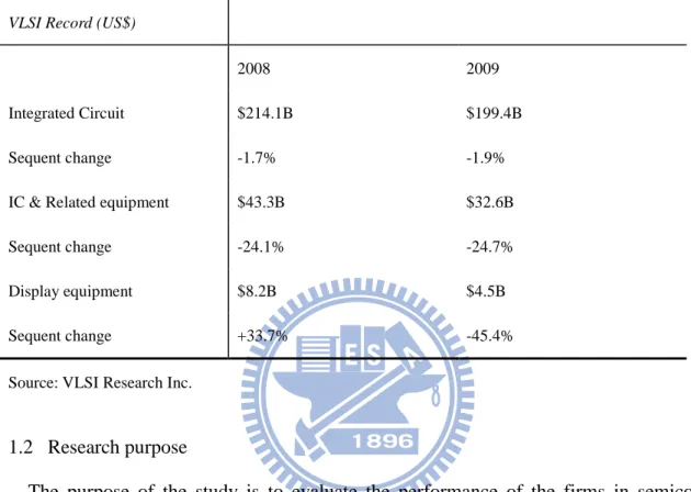
Table 1: VLSI annual sales by market segment VLSI Record (US$)

2008 2009

Integrated Circuit $214.1B $199.4B

Sequent change -1.7% -1.9%

IC & Related equipment $43.3B $32.6B

Sequent change -24.1% -24.7%

Display equipment $8.2B $4.5B

Sequent change +33.7% -45.4%

Source: VLSI Research Inc.

1.2 Research purpose

The purpose of the study is to evaluate the performance of the firms in semiconductor equipment industry. With the study, we can identify the frontier line of the industry, and find out the efficiency and non-efficiency firms. The financial capital market was seriously hit by the collapse of the giant banking institutions. Firms are hard to gain money from the capital market and the demand is contracted. The free cash flow is a key for sustainable operations. Many firms started cutting a lot of expenditure in operation cost and shortened the investment in production lines. By minimizing the input factors or maximizing the output factors, a non-efficiency firm can become an efficiency one. The study provides a reference for management teams to understand the behavior and performance of their competitors. Then they can lean from them to make right decisions and strategies to face the challenge in the future.

(11)

3

1.3 The trend of semiconductor market Demand:

According to the statistics from the Semiconductor Industry Association (SIA), global semiconductor sales began to decline in the 4th quarter of 2008 after six years of strong growth since 2001. The global financial crisis seriously hit the financial system and it caused many companies very hard to get financial support from financial market. Capacity addition has slowed and the trend and expected to continue into 2010.

The worldwide recession from the end of 2008 reduced the demand for semiconductors. The memory market was suffered in both prices and sales. For example, the average selling price of DRAM chip dropped sharply from US$3.81 in 2007 to US$1.5 in 2008, in response to significantly oversupply and inventory. The demand will remain poor as the financial crisis continues to hit the end-user industries, such as PC and mobile phone, which makes up about 60 % share of the demand for the semiconductor market.

The SIA projected that the global semiconductor sales in 2009 is around US$246.7 billion, resume to rise to US$264.9 billion in 2010, US$284.7 billion in 2011. The global sales listed by device type and region are list down in the table below.

(12)

4

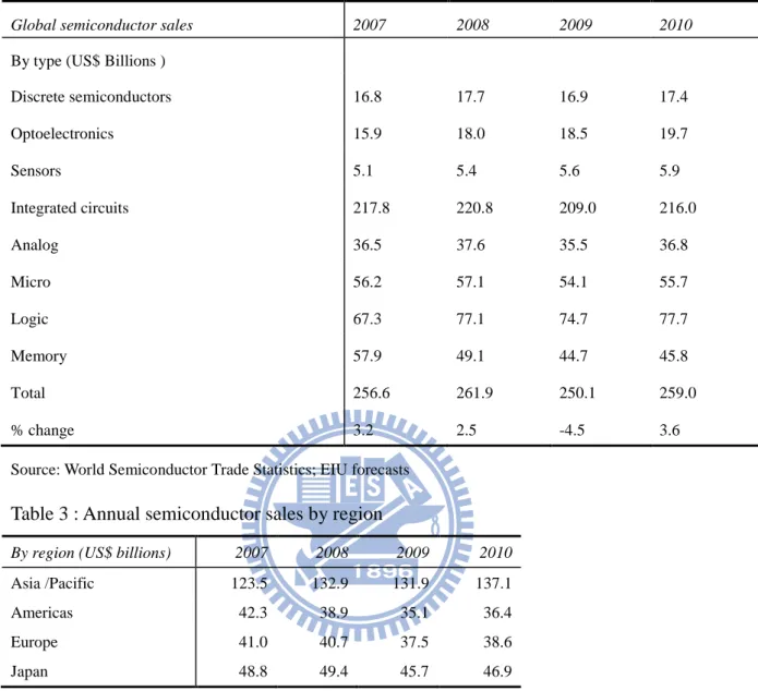
Table 2 : Annual global semiconductor sales by products

Global semiconductor sales 2007 2008 2009 2010

By type (US$ Billions )

Discrete semiconductors 16.8 17.7 16.9 17.4 Optoelectronics 15.9 18.0 18.5 19.7 Sensors 5.1 5.4 5.6 5.9 Integrated circuits 217.8 220.8 209.0 216.0 Analog 36.5 37.6 35.5 36.8 Micro 56.2 57.1 54.1 55.7 Logic 67.3 77.1 74.7 77.7 Memory 57.9 49.1 44.7 45.8 Total 256.6 261.9 250.1 259.0 % change 3.2 2.5 -4.5 3.6

Source: World Semiconductor Trade Statistics; EIU forecasts

Table 3 : Annual semiconductor sales by region

By region (US$ billions) 2007 2008 2009 2010

Asia /Pacific 123.5 132.9 131.9 137.1

Americas 42.3 38.9 35.1 36.4

Europe 41.0 40.7 37.5 38.6

Japan 48.8 49.4 45.7 46.9

Source: World Semiconductor Trade Statistics; EIU forecasts

Price:

As per the data from the Economist Intelligence Units which have tracked three main types of semiconductor prices, and the average selling price (ASP)of the integrated circuit from 2006, the ASP of IC tends to be much lower than the increasingly capacity and capability of flash memory, DRAM, and microprocessor. The ASP of the integrated circuit started to drop down from US$1.7 in 2007 due to the surplus capacity shrinks and over expand in inventory. The forecast expects the trend is downward until 2011 as the worldwide demand is contracted under recession and the supply side is still over capacity. Another force

(13)

5

may drive the price up. It is the US dollar currency. After the G20 meeting in 2009, the major industry countries decided to inject more money in the financial market. The inflation rate is a potential problem especially the weak US dollars that are widely used for international trading for raw materials, oil, and many industry products. The price change is list down in the below table.

Table 4 : Semiconductor annual average selling price(ASP) change

Semiconductor prices (US$/unit)

2006 2007 2008 2009 2010

IC average 1.56 1.70 0.70 0.50 0.50

% change -6.1 8.8 -58.8 -28.6 0.0

DRAM (all types) 3.58 1.50 3.81 1.10 1.02

% change -4.4 -58.1 154.0 -71.1 -7.3

Flash Memory 4.53 1.80 4.45 1.30 1.20

% change 9.4 -60.3 147.2 -70.8 -7.7

Microprocessor 96.37 100.00 39.40 26.80 28.90

% change -9.5 3.8 -60.6 -32.0 7.8

(14)

6

2. Literature review

2.1 Firm performance measurement

The issues of evaluating performance in firm level have been an important and interesting topics for researchers for a long time. A firm can be discriminated as excellent or non-excellent due to different criteria or indexes. One of the traditional ways to exam a firm’s performance or production efficiency is to measure its financial performance. Woo and Willard (1983) analyzed the 14 quantitative financial variables in the PIMS database. The 14 variables are ROI, ROS, growth in revenues, cash flow/investment, market share, market share gain, new product activities relative to competitors, direct cost relative to competitors, product quality relative to competitors, R&D expenditure in product and process, variations in ROI, percentage point change in ROI and cash flow/investment. The results show that profitability factors such as return on investment (ROI), return on sales (ROS), are important measurements in performance. Though there are inherent problems in ROI, it is the essential comprehensive representation of performance. However, this kind of measurements relied on the financial accounting data. Accounting data are historic. They reflect the firm’s short-term performance and only consider the stockholder’s benefit. Firms have to carefully manage and purchase right strategies to increase their ability to response to the changes in environment. For example, one may heavily invested in R&D expenditure for innovations to capture the business opportunity in the future. It hurt its short-term profitability and the performance was poor compared to its rival. Chakravarthy (1986) analyzed the computer industry from 1964 to 1983 in U.S. and demonstrated the inadequacy of traditional measurements that are based on a firm’s profitability for evaluating its strategy performance. Instead, Chakravarthy(1986) measured the quality of a firm’s transformation to discriminate the excellent and non-excellent firms. The transformation processes that a firm pursued have two different types: adaptive specialization and adaptive generalization. Adaptive specialization emphasizes

(15)

7

the power of a firm on profitably exploiting its current environment and generating a net surplus of the contribution to its stakeholders. Adaptive generalization focuses on the investment of a firm’s net surplus of slack resources for improving its ability to face the future challenge and uncertainty (Cyert and March, 1963). The eight slack variables are cash flow/investment ratio, sales by total asset, R&D by sales ratio, market to book value, sales per employee, dept by equity ratio, working capital by sales ratio, and dividend payout ratio.

Boulding and Staelin (1995) provided an approach to assess general effects of strategy actions on firm performance. Before one can confidently gain the strategy generalization, he has to address and answer the following five questions:

1. What allows a firm to sustain strategy relationship in face of the competitive reactions? 2. Is it possible to find out the direction of causality in strategy relationship?

3. Can one identify the unobserved factors that influence firm performance and they correlate to strategy actions?

4. Are the strategy relationships measurable?

5. Are the strategy relationships unique to a particular firm? Or they are generalized over a wide range of conditions?

Empirically studying of the 2177 strategic business units for 4 years data in the PIMS (Profit Impact of Marketing Strategy) database, Boulding and Staelin concluded that the investment in R&D has positive effect on firm performance. The firms, which have high ability and motivation to leverage R&D asset, can increase the demand-side returns.

(16)

8

2.2 Empirical applications

Zhu (2000) provides a two stages model to evaluate the Fortune 500 firms in 1996. He selected eight financial variables which are provided by the Fortune magazine: number of employee, total asset, stockholder’s equity, revenue, profits, market value, total return to investors, and earnings per share instead of using total revenue as a single index for ranking firms. The total efficiency of a firm can be decomposed by two stages by adopted these eight variables. Stage 1 considered the ability of a firm to make profitability. Stage 2 uses the output factors in stage 1 as input factors to measure the performance of a firm to make marketability from yhe view of investors. Then stage 3 evaluates the total performance. Empirical results showed that revenue-top-ranked firms do not necessarily have top-ranked performance in terms of profitability and marketability.

Tsai et al. (2006) reconcile diverse efficiency measures to characterize the productivity efficiency of 39 Forbes 2000 ranked global telecom firms. Empirical results indicated that top-ranked Forbes telecom firms are not the same as those having top-ranked OTE (CRS TE). The study also showed that Asia-Pacific telecom firms have better OTE than those in Europe and America but the differences are not significant. Another interesting found is that the stated-owned firms show relative high efficiency than privatized telecoms (except China) because they provide full service (fixed-line, mobile, and internet).

Chen et al. (2006) evaluated six high-tech industries: semiconductor, computer, communications, photo-electronics, precision equipment, and biotech in Taiwan’s Hsin Chu Science Park. Empirical results show that the computer and semiconductor industry have the best performance in OTE while the other four industries are operated in inefficiency. Since the computer and semiconductor industries are the two major government supported policies and have had allocated many resources on them, the results confirmed that the investment were in

(17)

9

the right direction.

Wong et al. (2007) applied two DEA model: technical efficiency and cost efficiency to evaluate the performance in supply chain. Fifty semiconductor firms listed in the database of Penang Development Corporation, Malaysia, were selected to be decision-making units (DMUs). The results indicated that not all technical efficiency firms are also al-locative efficient. The opportunity cost derived from the model combining with the scenario analysis on the mix input allocation can help manage do better decision for resources allocation and planning.

Hung et al. (2008) used the DEA approach with the classical radial measure, non-radial efficiency measure and efficiency achievement measure to characterize the productivity efficiency of the IC packaging/testing firms in Taiwan. The results showed that the inefficiencies in OTE of these firms are primarily due to pure technical (VRS TE) inefficiencies rather than scale inefficiencies. Further mergers and acquisitions in this industry are good business strategy to correct the scale inefficiency problem.

The input and output variables selected by the above papers are summarized in the below tale.

(18)

10

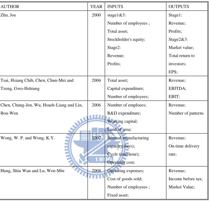
Table 5: Summary of Input / Output variables

AUTHOR YEAR INPUTS OUTPUTS

Zhu, Joe 2000 stage1&3:

Number of employees ; Total asset; Stockholder's equity; Stage2: Revenue; Profits; Stage1: Revenue; Profits; Stage2&3: Market value; Total return to investors; EPS; Tsai, Hsiang Chih, Chen, Chun-Mei and

Tzeng, Gwo-Hshiung 2006 Total asset; Capital expenditure; Number of employees; Revenue; EBITDA; EBIT; Chen, Chung-Jen, Wu, Hsueh-Liang and Lin,

Bou-Wen 2006 Number of emploees; R&D expenditure; Working capital; Land of area; Revenue; Number of patterns

Wong, W. P. and Wong, K.Y. 2007 Internal manufacturing capacity(days); Cycle time(hour); Operating cost; Revenue; On-time delivery rate;

Hung, Shiu Wan and Lu, Wen-Min 2008 Operating expenses; Cost of goods sold; Number of employees ; Fixed asset;

Revenue;

Income before tax; Market Value;

Capital expenditure (CAPEX) is expense used for company to purchase newly physical asset or maintain the assets’ current condition. It may include from factory roof to production equipments. The items counted in CAPEX are different from firms to firms. Adopted CAPEX as an input variable may cause large variation in our results. EBITDA is net income with interest, taxes, depreciation, and amortization added back to it. The disadvantage is the same with CAPEX. It’s non-GAAP measure that allows firms to manipulate numbers.

(19)

11

3. Analytical Framework and Methodology

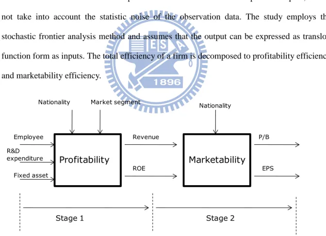
3.1 Analytical framework and hypothesis

This study adopted the concept of the two stage performance model proposed by Zhu (2000). A firm’s performance can be measured in two dimensions. Stage 1 measures the efficiency to leverage its resources to generate profits. Stage 2 takes into account the value and potential of a firm from investors’ view. According to the literature review, the investment on research and development is very important on firm’s performance in hi-tech industry. It was selected as one of the inputs in the stage1. There are parametric and non-parametric methods to evaluate firm level performance. Though using DEA (data envelopment analysis) method does not need to know the specific function forms between outputs and inputs, it does not take into account the statistic noise of the observation data. The study employs the stochastic frontier analysis method and assumes that the output can be expressed as translog function form as inputs. The total efficiency of a firm is decomposed to profitability efficiency and marketability efficiency.

Figure 1: Research model

Profitability Marketability Employee R&D expenditure Fixed asset Revenue ROE P/B EPS Nationality Market segment _Nationality

(20)

12

And defines the

Total efficiency = (Profitability efficiency) x (Marketability efficiency). (3.1) The definitions and explanation of these variables are listed on the below table 6. Table 6: Definition of variables

Variable Definition

Stage1:Inputs

Employee The total number of employees in the year –end.

R&D Firm’s investment on research and development activities. Fixed asset Firm’s long-term, tangible asset held for business use, such as

equipment, real estate, and furniture. Stage1:Outputs

Revenue Total amount of money received by the company for goods sold or services provided.

ROE The amount of net income returned as a percentage of shareholders equity.

Stage 2:Inputs The same as the outputs in stage1. Stage2:Outputs

P/B Price to book ratio. Firm’s share price divided by its book value per share. The value is calculated base on the data on 12/31.

(21)

13

Hypothesis:

As we are interesting in how the performances of these firms are affected by the two environment factors? We set up the following two hypothesizes:

H1: The performances of Japanese firms are different from EU/US firms’. H2: The performance of the front-end firms and the back-end are different.

3.2 Data selection and Collection

The study uses the firms (DMU) listed in the library of the VLSI research Inc. There are 32 cross-sectional DMUs in each period, giving the total 96 DMUs. The numbers of input and output factors are financial release and withdraw from Thomson’s data stream on- line database from year 2006 to 2008. All numbers are expressed in US dollar in thousands and the yen to U.S. dollar currency is the annual average number provided by Bank of Japan. In order to avoid the negative value for logarithm calculating, then we replace ROE as ROE+10, and EPS as EPS+3 for all periods. Since the data covers three years, so we deflated the financial variables by CPI ( CPI=1, y2006)

All the input and output data are derived from Thomson Financial / Data stream on-line database.

Table 7: Currency

Year USD to JPY* CPI( 2006=1)** 2006 116.20 NA

2007 117.60 2.85% 2008 102.46 5.85%

Source: * Foreign exchange rate on 11/29/2008: Bank of Japan. ** Data derived from Inflationdata.com

(22)

14

3.3 The stochastic frontier model for panel data

Consider a single output “y” which can be expressed as a production function of N inputs:

y= f( , …, ), (3.2)

Where y is the dependant variable, the (n=1, 2… N) is explanatory variable. A translog production function form has been widely employed by researchers. y=exp [ + ln + ln ln ] (3.3) If set all = 0, then the Cobb-Douglas production function is obtained.

Aigner et al., (1977), Meeusen and Van Broeck (1977), both independently proposed a stochastic frontier model which assumed that the technical inefficiency for an individual firm is time invariant.

An extended model proposed by Battese and Coelli(1992,1995) allows us to deal with the technical inefficiency term in time –varying levels. Since the technical inefficiency term is not constant, it’s important to seek how the variation is explanatory by appropriate environmental variables. Some early researchers like Pitt and Lee ( 1981) employed a so called two stages model. The first stage contains estimating the technical inefficiency in stochastic frontier model without considering the environmental variables. The second stage is to regress the predicted technical inefficient effects on the environmental variables. However this approach violates the consistent assumptions regarding to the identical distribution of the technical efficiency variation in these two estimation stages. To avoid this inconsistent problem, Battese and Coelli (1992, 1995) introduced a one stage method for dealing with panel data. The efficiency effects of the observable environmental variables are directed incorporated into the stochastic frontier model.

(23)

15

Consider a single output y in the i th firm (i=1.., N) and at period t (t=1.., T),

, (3.4)

(3.5)

Where

1 x k) vector of inputs.

: Statistic error of the normal distribution. It can be negative or positive.

: Non-negative random variable associated with technical inefficiency of production.

It is truncated at zero of the normal distribution, N~ ( .

: (k x 1) vector of unknown parameters to be estimated.

: (1 x m) vector of explanatory variables associated with technical inefficiency of

production of firms over time.

: (m x 1) vector of unknown coefficients.

: defined by the truncation of the normal distribution, N~ (0,

Equation (3.4) specifies the stochastic production function as a form of the original function. Equation (3.5) specifies the technical inefficiency effects. The s which are assumed to be a function of the explanatory environmental variables, and the unknown vector of coefficients,

The method of maximum likelihood is proposed for simultaneous estimation of these parameters of the stochastic frontier model. The parameters, and / ( , defined by Battese and Corra (1977), are also obtained with the calculation of the maximum likelihood estimation.

(24)

16

3.4 Distance Function

Equation (3.3) is a case of single output production function. In reality, the majority of econometric cases are multiple outputs production problem with a set of combinations of multiple inputs. A distance function approach was adopted by many researchers (e.g. Lovell et al., 1994).

The output distance function defined by Shephard (1970) is as below:

Do(x, y)= min { (3.6) Where P(x) ={y ; x (3.7)

If Do(x, y) <1, it means that y belongs to production possibility set of y P(x), and if Do(x, y) =1, it means that y is on the frontier of the production possibility set of P(x). Then the stochastic distance function form can be specified as:

Do(x, y) = f (x, y, ) (3.8)

Where is an unknown parameters to be estimated, and is a random variable to catch the statistical noise and measurement error. ~N (0, ).

Many researchers (e.g. Grosskopf et al., 1996; Coelli and Perelman, 2000) have employed the translog formula form as the f(.) in equation (3.8) for study. Consider the nth firm in the sample, the translog distance function with M outputs and J inputs can be specified as: (3.9) The restriction of linear homogeneity in outputs requires:

(25)

17

The restriction of symmetry requires:

(3.11)

To solve the unobservable dependent variable , we impose the linear homogeneity in outputs. Equation (3.9) becomes:

(3.12) where

Then equation (3.12) can be rewritten as:

Replace . And is assumed to be iid of and truncated at zero of ). The predicted value of can’t be obtained directed because it is only part of the composed error term, . Then the predicted value of can be predicted by given the condition of

(26)

18

(3.14)

The parameters in Equation (3.13) can be estimated by using the maximum likelihood method [Coelli and Perelman, 2000].

(27)

19

4. Empirical Results

4.1. Descriptive statistic

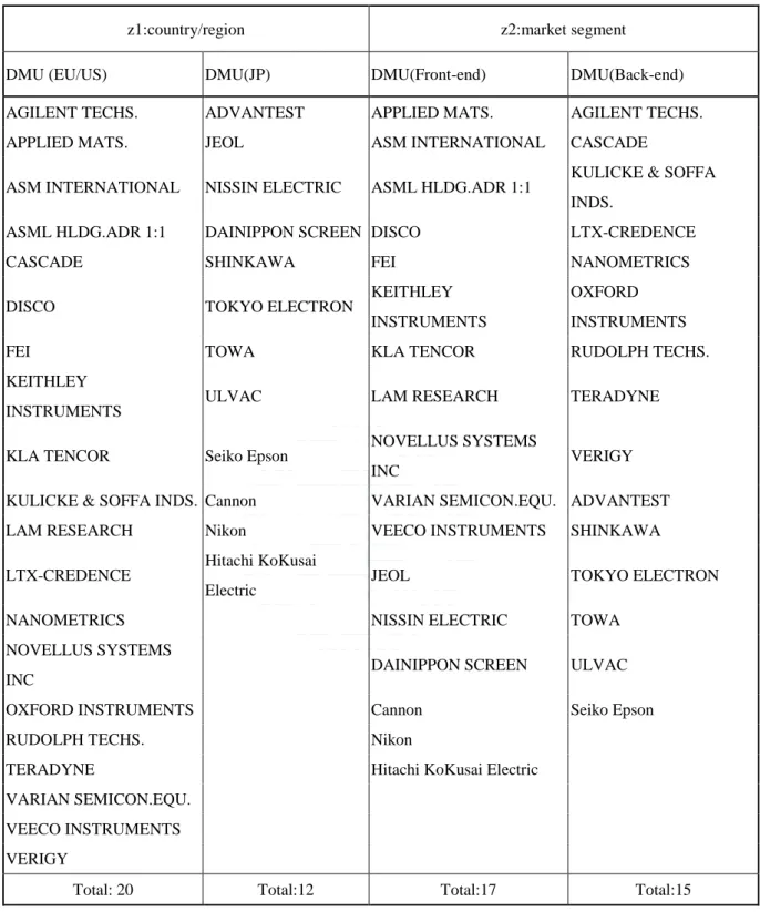
This study is targeted at 20 Japanese firms, and 12 EU/US firms, giving total 32 cross-sectional DMUs. These 32 DMUs can be classified into two categories: market segmentation and nationality. The market of the semiconductor equipment industry is typically divided into two segments: front-end and back-end, according to its different application. For considering the other environmental effect: nationalities, these 32 DMUs are also classified into two groups by their ownership: EU/US, and JP. In our model, two stages approach is employing for evaluating the performance. The seven put/output factors are number of employee, fixed asset, R&D expenditure, revenue, ROE, EPS, and price to book ratio; and the two environmental variables are z1(country/region), and z2(market segment). The period is from year 2006 to 2008, giving total 672 observations. Table 8 shows the DMU’s classification by two environmental variables. Table 9 is the descriptive statistics of the sample sets. Table 10 provides us a ranking list of these DMUs by their revenue in each period.

(28)

20

Table 8: DMUs classified by environmental variables

z1:country/region z2:market segment

DMU (EU/US) DMU(JP) DMU(Front-end) DMU(Back-end)

AGILENT TECHS. ADVANTEST APPLIED MATS. AGILENT TECHS. APPLIED MATS. JEOL ASM INTERNATIONAL CASCADE ASM INTERNATIONAL NISSIN ELECTRIC ASML HLDG.ADR 1:1 KULICKE & SOFFA

INDS.

ASML HLDG.ADR 1:1 DAINIPPON SCREEN DISCO LTX-CREDENCE CASCADE SHINKAWA FEI NANOMETRICS DISCO TOKYO ELECTRON KEITHLEY

INSTRUMENTS

OXFORD

INSTRUMENTS

FEI TOWA KLA TENCOR RUDOLPH TECHS. KEITHLEY

INSTRUMENTS

ULVAC LAM RESEARCH TERADYNE

KLA TENCOR Seiko Epson NOVELLUS SYSTEMS INC

VERIGY KULICKE & SOFFA INDS. Cannon VARIAN SEMICON.EQU. ADVANTEST LAM RESEARCH Nikon VEECO INSTRUMENTS SHINKAWA LTX-CREDENCE

Hitachi KoKusai

Electric JEOL TOKYO ELECTRON NANOMETRICS NISSIN ELECTRIC TOWA NOVELLUS SYSTEMS

INC DAINIPPON SCREEN ULVAC

OXFORD INSTRUMENTS Cannon Seiko Epson

RUDOLPH TECHS. Nikon

TERADYNE Hitachi KoKusai Electric

VARIAN SEMICON.EQU.

VEECO INSTRUMENTS

VERIGY

(29)

21

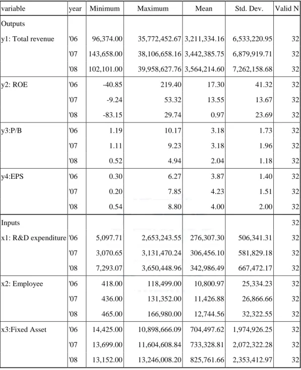
Table 9: Descriptive statistics of the input/output variables

variable year Minimum Maximum Mean Std. Dev. Valid N

Outputs

y1: Total revenue '06 96,374.00 35,772,452.67 3,211,334.16 6,533,220.95 32 '07 143,658.00 38,106,658.16 3,442,385.75 6,879,919.71 32 '08 102,101.00 39,958,627.76 3,564,214.60 7,262,158.68 32 y2: ROE '06 -40.85 219.40 17.30 41.32 32 '07 -9.24 53.32 13.55 13.67 32 '08 -83.15 29.74 0.97 23.69 32 y3:P/B '06 1.19 10.17 3.18 1.73 32 '07 1.11 9.23 3.18 1.96 32 '08 0.52 4.94 2.04 1.18 32 y4:EPS '06 0.30 6.27 3.87 1.40 32 '07 0.20 7.85 4.23 1.51 32 '08 0.54 8.80 4.00 2.00 32 Inputs 32 x1: R&D expenditure '06 5,097.71 2,653,243.55 276,307.30 506,341.31 32 '07 3,070.65 3,131,470.24 306,456.10 581,829.18 32 '08 7,293.07 3,650,448.96 342,986.49 667,472.17 32 x2: Employee '06 418.00 118,499.00 10,800.97 25,334.23 32 '07 436.00 131,352.00 11,426.88 26,866.66 32 '08 465.00 166,980.00 12,744.56 32,322.55 32 x3:Fixed Asset '06 14,425.00 10,898,666.09 704,497.62 1,974,926.25 32 '07 13,699.00 11,604,608.84 733,328.81 2,072,322.28 32 '08 13,152.00 13,246,008.20 825,761.66 2,353,412.97 32

Notes: Total revenue, R&D expenditure, and fixed asset are numbers in $1000US. EPS is number in $US. The numbers of y1, y2, y4, x1, and x3 are adjusted by annual inflation rate for each period.

(30)

22

Table 10: Annual revenue ranking Rankin

g

2006 2007 2008

1 Cannon Cannon Cannon 2 Seiko Epson Seiko Epson Seiko Epson 3 APPLIED MATS. APPLIED MATS. Nikon

4 Nikon TOKYO ELECTRON TOKYO ELECTRON 5 TOKYO ELECTRON Nikon APPLIED MATS. 6 AGILENT TECHS. AGILENT TECHS. AGILENT TECHS. 7 ASML HLDG.ADR 1:1 ASML HLDG.ADR 1:1 ASML HLDG.ADR 1:1 8 DAINIPPON SCREEN MNFG. KLA TENCOR DAINIPPON SCREEN MNFG. 9 ADVANTEST DAINIPPON SCREEN MNFG. KLA TENCOR 10 KLA TENCOR LAM RESEARCH LAM RESEARCH 11 ULVAC ULVAC ULVAC 12 NOVELLUS SYSTEMS INC ADVANTEST Hitachi KoKusai Electric 13 LAM RESEARCH Hitachi KoKusai Electric ADVANTEST 14 TERADYNE NOVELLUS SYSTEMS INC TERADYNE 15 Hitachi KoKusai Electric ASM INTERNATIONAL

(NAS)

ASM INTERNATIONAL (NAS)

16 ASM INTERNATIONAL (NAS)

TERADYNE NISSIN ELECTRIC 17 JEOL VARIAN SEMICON.EQU. NOVELLUS SYSTEMS INC 18 VERIGY JEOL JEOL 19 NISSIN ELECTRIC NISSIN ELECTRIC DISCO 20 VARIAN SEMICON.EQU. VERIGY VARIAN SEMICON.EQU. 21 KULICKE & SOFFA INDS. DISCO VERIGY 22 DISCO KULICKE & SOFFA INDS. FEI 23 FEI FEI CASCADE 24 CASCADE CASCADE VEECO INSTRUMENTS 25 VEECO INSTRUMENTS VEECO INSTRUMENTS KULICKE & SOFFA INDS. 26 SHINKAWA SHINKAWA SHINKAWA 27 LTX-CREDENCE TOWA TOWA 28 RUDOLPH TECHS. OXFORD INSTRUMENTS OXFORD INSTRUMENTS 29 TOWA RUDOLPH TECHS. KEITHLEY INSTRUMENTS 30 OXFORD INSTRUMENTS LTX-CREDENCE LTX-CREDENCE 31 KEITHLEY INSTRUMENTS NANOMETRICS RUDOLPH TECHS. 32 NANOMETRICS KEITHLEY INSTRUMENTS NANOMETRICS

(31)

23

4.2. Coefficient and TE

Following, we describe the distance production function forms applied in our model. Stage 1: Profitability efficiency

According to the equation (3.10), the distance function at stage 1 can be specified as below:

(4.1)

And the external environmental effects on the technical inefficiency can be specified as: (4.2)

(32)

24

Stage 2: Marketability efficiency

The distance function at stage 2 can be specified as:

(4.3)

And the external environmental effects on the technical inefficiency at stage 2 can be specified as:

(4.4)

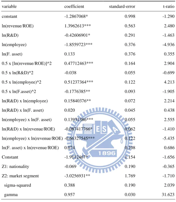
Base on the equation 4.1~4.4 described above, a maximum likelihood method is employed to estimate the unknown coefficients. The software program: Frontier 4.1 which is developed by Tim Coelli has been widely applied for calculation. The results of the estimated unknown parameters at stage1 are showed on Table 11

(33)

25

Table 11: Coefficients at stage1 (profitability)

Stage1:Profitability

variable coefficient standard-error t-ratio

constant -1.2867068* 0.998 -1.290 ln(revenue/ROE) 1.3962613*** 0.563 2.480 ln(R&D) -0.42606901* 0.291 -1.463 ln(employee) -1.8559723*** 0.376 -4.936 ln(F. asset) 0.133 0.376 0.355 0.5 x [ln(revenue/ROE)]^2 0.47712463*** 0.164 2.904 0.5 x ln(R&D)^2 -0.038 0.055 -0.699 0.5 x ln(employee)^2 0.51237364*** 0.122 4.213 0.5 x ln(F.asset)^2 -0.1776385** 0.093 -1.905 ln(R&D) x ln(employee) 0.15840376** 0.072 2.214 ln(R&D) x ln(F. asset) 0.020 0.045 0.438 ln(employee) x ln(F. asset) 0.13931386*** 0.055 2.555 ln(R&D) x ln(revenue/ROE) -0.087417766* 0.062 -1.410 ln(employee) x ln(revenue/ROE) -0.66327545*** 0.122 -5.435 ln(F. asset) x ln(revenue/ROE) 0.074 0.108 0.686 Constant -1.9112467* 1.154 -1.656 Z1: nationality -0.069 0.190 -0.365 Z2: market segment -3.0256931** 1.769 -1.710 sigma-squared 0.388 0.190 2.039 gamma 0.957 0.030 31.623 *Significant at 10 % level **Significant at 5 % level ***Significant at 1 % level

Note: Coefficients are calculated under homogeneity condition. N=96. log likelihood function = 0.34238212E+02

The gamma value is 0.957 means that 95.7 % of the error composition term is due to technical inefficiency, and 4.3% is due to statistic noise. The coefficient of the environmental variable is -3.0256931, giving a significantly negative effect on technical inefficiency .

(34)

26

However the coefficient of z1 is -0.069 and the t-ratio indicates that the result is not significant at 10% level. This result shows that by giving the same inputs, EU/US firms have same efficiency to make profits as Japanese firms.Table 12 is the estimated results of unknown parameters at stage 2.

Table 12: Coefficients at stage 2 (Marketability)

Stage 2: Marketability

variable coefficient standard-error t-ratio

constant -11.412342* 7.326 -1.558 ln(EPS/PB) -0.030 0.667 -0.045 ln(Revenue) -19.666486* 12.995 -1.513 ln(ROE) 21.098353* 13.590 1.552 0.5 x [ln(EPS/PB)]^2 0.337 0.094 3.596 0.5 x ln(Revenue)^2 -67.172 80.663 -0.833 0.5 x ln(ROE)^2 208.17297** 92.206 2.258 ln(Revenue) x ln(ROE) -70.549 71.493 -0.987 ln(Revenue) x ln(EPS/PB) -31.278309** 17.447 -1.793 ln(ROE) x ln(EPS/PB) 31.317044** 17.446 1.795 Constant 0.311 0.277 1.121 Z2:market segment -0.17942971** 0.093 -1.938 sigma-squared 0.115 0.019 6.024 gamma 0.739 0.261 1.453 *Significant at 10 % level **Significant at 5 % level ***Significant at 1 % level

Note: Coefficients are calculated under homogeneity condition. N=96. log likelihood function = -0.29630460E+02

The gamma value at stage 2 is 0.739 which means that 73.9% of the error composition term is due to technical inefficiency, and 22.1% is due to statistic noise. The coefficient of the external environmental variable is -0.17942971, giving a significantly negative effect on the technical inefficiency . The t-ratio indicates that the result is significant at 5 % level.

(35)

27

Base on these results, the model can be modified as:

Figure 2: Modified research model

The values of the technical efficiency of the firms, at each stage are shown at Table 13. Profitability Marketability Employee R&D expenditure Fixed asset Revenue ROE P/B EPS Market segment Nationality Stage 1 Stage 2

(36)

28

Table 13: Annual technical efficiency at each stage

year 2006 2007 2008

DMU TE1 TE2 TE t TE1 TE2 TE t TE1 TE2 TE t

1 AGILENT TECHS. 0.6434 0.4901 0.3153 0.9328 0.5076 0.4735 0.9170 0.5190 0.4759 2 APPLIED MATS. 0.9547 0.5914 0.5646 0.9366 0.6279 0.5881 0.9620 0.6622 0.6371 3 ASM INTERNATIONAL 0.9403 0.5643 0.5306 0.9191 0.5695 0.5234 0.9259 0.6594 0.6106 4 ASML HLDG.ADR 1:1 0.9177 0.5622 0.5159 0.9142 0.5625 0.5142 0.9351 0.6159 0.5759 5 CASCADE 0.8109 0.4436 0.3597 0.8301 0.4327 0.3592 0.8392 0.4095 0.3437 6 DISCO 0.9137 0.5474 0.5002 0.9220 0.5240 0.4831 0.9219 0.5454 0.5028 7 FEI 0.9307 0.6075 0.5654 0.9112 0.5858 0.5338 0.9496 0.6683 0.6346 8 KEITHLEY INSTRUMENTS 0.9367 0.5754 0.5390 0.9549 0.5812 0.5550 0.9536 0.6329 0.6035 9 KLA TENCOR 0.9594 0.6242 0.5989 0.9456 0.5482 0.5184 0.9579 0.5686 0.5446 10 KULICKE & SOFFA INDS. 0.3952 0.4041 0.1597 0.8759 0.4124 0.3612 0.9433 0.5235 0.4938 11 LAM RESEARCH 0.9392 0.5402 0.5073 0.8385 0.4849 0.4066 0.9048 0.5279 0.4776 12 LTX-CREDENCE 0.7815 0.4775 0.3732 0.9339 0.4699 0.4388 0.9299 0.4896 0.4552 13 NANOMETRICS 0.9324 0.5304 0.4945 0.8701 0.5242 0.4561 0.9533 0.5343 0.5094 14 NOVELLUS SYSTEMS INC 0.9483 0.5849 0.5546 0.9464 0.5958 0.5639 0.9672 0.7828 0.7571 15 OXFORD INSTRUMENTS 0.9350 0.4904 0.4585 0.9237 0.4645 0.4291 0.9187 0.3516 0.3230 16 RUDOLPH TECHS. 0.7815 0.5056 0.3951 0.8994 0.5091 0.4578 0.9509 0.5965 0.5672 17 TERADYNE 0.9116 0.5688 0.5186 0.9349 0.5896 0.5512 0.9738 0.7992 0.7783 18 VARIAN SEMICON.EQU. 0.9192 0.5985 0.5501 0.8724 0.4876 0.4254 0.8643 0.6071 0.5247 19 VEECO INSTRUMENTS 0.9341 0.5443 0.5084 0.9392 0.5506 0.5171 0.9538 0.7890 0.7525 20 VERIGY 0.8855 0.6007 0.5319 0.8599 0.5132 0.4414 0.8991 0.5899 0.5304 21 ADVANTEST 0.8683 0.6198 0.5381 0.9152 0.6563 0.6006 0.9284 0.7279 0.6758 22 JEOL 0.9425 0.8405 0.7922 0.9396 0.8299 0.7798 0.9414 0.8624 0.8119 23 NISSIN ELECTRIC 0.9490 0.8201 0.7783 0.9455 0.8540 0.8075 0.9456 0.8462 0.8002 24 DAINIPPON SCREEN 0.9152 0.7834 0.7170 0.9153 0.8088 0.7403 0.9017 0.8640 0.7791 25 SHINKAWA 0.6243 0.6696 0.4180 0.6162 0.6714 0.4137 0.7306 0.7386 0.5396 26 TOKYO ELECTRON 0.8860 0.6616 0.5862 0.7973 0.6040 0.4816 0.8602 0.5903 0.5077 27 TOWA 0.9587 0.8144 0.7807 0.8665 0.6923 0.5999 0.8599 0.6869 0.5906 28 ULVAC 0.8538 0.7057 0.6025 0.9108 0.7142 0.6504 0.9308 0.7646 0.7117 29 Seiko Epson 0.9226 0.8797 0.8115 0.9053 0.8332 0.7544 0.9196 0.7880 0.7247 30 Cannon 0.9374 0.7946 0.7449 0.9144 0.7939 0.7259 0.9101 0.8086 0.7359 31 Nikon 0.9552 0.8154 0.7788 0.9595 0.7950 0.7628 0.9557 0.7516 0.7183 32 Hitachi KoKusai Electric 0.9469 0.8328 0.7886 0.9351 0.8173 0.7643 0.9467 0.8269 0.7829 mean Industry 0.8791 0.6278 0.5519 0.8994 0.6129 0.5512 0.9204 0.6603 0.6077 mean EU/US DMUs 0.8686 0.5426 0.4713 0.9080 0.5271 0.4786 0.9311 0.5936 0.5527 mean JAPAN DMUs 0.8967 0.7698 0.6903 0.8851 0.7559 0.6690 0.9026 0.7713 0.6962 mean Front-end DMUs 0.9377 0.6604 0.6193 0.9241 0.6480 0.5988 0.9351 0.7070 0.6611 mean Back-end DMUs 0.8127 0.5908 0.4801 0.8715 0.5730 0.4993 0.9036 0.6073 0.5488

(37)

29

4.3 Efficiency Change Index

The efficiency change from period “s” to period “t” is defined as:

[Coelli et al., (2005)] (4.5) If efficiency change >1, the efficiency is improved.

If efficiency change <1, the efficiency becomes worse. If efficiency change=1, the efficiency keeps constant.

Then the yearly sequential efficiency change can be obtained by using equation 4.5.

From the results on Table 14, 15 and 16, one can have a whole picture about the trend in this industry.

Table 14: Technical efficiency change index at stage 1 (profitability)

Year 2007 2008 Industry 1.0231 1.0233 by nationality EU/US DMUs 1.0455 1.0254 JAPAN DMUs 0.9871 1.0198 by market segment Front-end DMUs 0.9855 1.0120 Back-end DMUs 1.0723 1.0369

At stage 1, the “industry” efficiency change is greater than 1 in 2007 and 2008, means that capability to make profits in the whole semiconductor equipment industry are improved in this three years period. We may say that the market is on the upward cycle. The values of the EU/US firms and of the back-end firms are also greater than 1 means that performance of these specific firms are also continued improved. In contrast, the values of Japanese firms and of the front-end firms are smaller than 1 in 2007, but returns back to greater than 1 in 2008. It means that these firms did not perform well from year 2006 to 2007, but the performances are recovered back in 2008.

(38)

30

Table 15: Technical efficiency change index at stage 2 (marketability)

Year 2007 2008 Industry 0.9762 1.0774 by nationality EU/US DMUs 0.9714 1.1263 JAPAN DMUs 0.9819 1.0205 by market segment Front-end DMUs 0.9813 1.0910 Back-end DMUs 0.9698 1.0599

At stage 2, the “industry” efficiency change is slightly down to 0.9762 in 2007 but returns to 1.0774 in 2008, means that the efficiency of the whole industry dropped down in 2007 but got improved in 2008. We also observed the similar pattern whether the firms are classified by nationality or market segment.

Table 16: Total Efficiency Change Index

Year 2007 2008 Industry 0.9988 1.1025 by nationality EU/US DMUs 1.0156 1.1549 JAPAN DMUs 0.9692 1.0407 by market segment Front-end DMUs 0.9671 1.1040 Back-end DMUs 1.0399 1.0990

The total “industry” efficiency is slightly down to 0.9988 in 2007, but returns back to 1.1025 in 2008. However we see different pattern for the firms which are classified as EU/US firms or back-end equipment firms. The values of efficiency change for these firms kept greater than 1 for all 3 years; mean that total efficiency of these specific firms are continued improving year by year even the industry is slowly down in 2007.

(39)

31

4.4. Summary and Hypothesis test

To understand deeply about how these specific firms perform and the effect of the environmental variables, we now plotted the DMU’s average TE at each stage(Fig.3~Fig.8).

Figure 3: Annual TE (classified by nationality) at stage1

At stage 1(Fig.3), the performance improvement of the EU/US firms overcame the performance drops down in the Japanese firms from 2006 to 2007. The performance of the Japanese firms is under 3- years’ average level.

At stage 2(Fig.4), the marketability efficiency of the Japanese firms is much better than the EU/US firms for our analysis period. And it is behind the average level. From the comparison of the EU/US firms at stage 1 and 2, we found that the EU/US firms have a good efficiency to generate profits but failed to get respect from investors (marketability efficiency). 0.8 0.9 1.0 2006 2007 2008 year

Stage1:Profitability (by nationality)

Industry EU/US JAPAN 3-years ave.(Industry) TE

(40)

32

Figure 4: Annual TE (classified by nationality) at stage 2

By definition, in order to obtain the total efficiency, we multiply the profitability efficiency and the marketability efficiency. Then the results are plotted on Fig.5.

The figure shows that the total efficiency of the Japanese firms is better than the EU/US firms. We begin to test our hypothesis#1.

H1: The performances of Japanese firms are different from EU/US firms’.

Figure 5: Annual total TE (classified by nationality) 0.4 0.5 0.6 0.7 0.8 2006 2007 2008 TE year

Stage2:Marketability (by nationality)

Industry EU/US JAPAN 3-years ave.(Industry) 0.4 0.5 0.6 0.7 0.8 2006 2007 2008 TE year

Total efficiency (by nationality)

Industry EU/US JAPAN 3-years ave.(Industry)

(41)

33

A Mann-Whitney U test has been widely applied for this kind of Non-parametric Statistics. From the results shown on Table 17, we can conclude our hypothesis#1 as:

H1: The total efficiencies of Japanese firms are significantly higher than the EU/US firms (p<0.01).

Table 17: Mann-Whitney U test for Hypothesis#1

N1 N2 U P(two-tailed) P(one-tailed) 60 36 1876.5 <2 e-06 <2 e-06

Normal approx, Z=6.02787 1.661376e-09*** 8.30688e-10*** Note: ***significant at 1 % level

(42)

34

Below we discuss and summarize the performance in different market segment.

As the results shown on Fig.6, at stage 1, the front-end firms have better capability to make profits than the back-end firms. However the performance improvement which comes from the Japanese firms drives the industry continuously improving in our analysis period.

Figure 6: Annual TE (classified by market segment) at stage 1

0.7 0.8 0.9 1.0 2006 2007 2008 TE year Stage1:Profitability (by market segment)

Industry Front-end Back-end 3-years ave.(Industry)

(43)

35

At stage 2(Fig.7), the performance of the front-end firms is better than the back-end firms. And the average profitability efficiency for industry is slightly gone down in 2007.

Figure 7: Annual TE (classified by market segment) at stage 2

Upon our definition of the total efficiency, the final result is showed on Fig.8.

From the figure, we found that the total performance of the front-end firms is better than the back-end firms. We begin to test our hypothesis#2.

H2: The performance of the front-end firms and the back-end are different.

0.4 0.5 0.6 0.7 0.8 2006 2007 2008 TE year Stage2:Marketability (by market segment)

Industry

Front-end

Back-end

3-years ave.(Industry)

(44)

36

Figure 8: Annual total TE (classified by market segment)

The results of the Mann-Whitney U test are showed on Table 18. So we concluded that the hypothesis#2 as:

H2: The total efficiencies of the front-end equipments firms are significantly higher than the back-end equipments firms (p<0.01).

Table 18: Mann-Whitney U test for Hypothesis#2

N1 N2 U P(two-tailed) P(one-tailed) 51 45 1699.5 <2e-05*** <1e-05*** Normal approx, Z=4.05277 5.06136e-05*** 2.53068e-05*** Note: ***significant at 1% level

0.4 0.5 0.6 0.7 2006 2007 2008 TE year Total efficiency (by market segment)

Industry Front-end Back-end 3-years ave.(Industry)

(45)

37

5. Conclusion

As the cycle of the semiconductor market becomes shorter and shorter, it’s important to for firm to make right strategy to survive and to be competitive in this market. The empirical results show that the efficiencies of the EU/US firms to generate profits can catch the cycle of the market. They kept improving their profitability as the market grew. Usually, the EU/US firms employ more active operating strategy than Japanese firms. They expanded their production capacity and men power quickly as the market grows. In contrary, they lay off employees and close their factory as the market constricts. Japanese firms maintain their capability and cost conservatively. The total efficiencies of Japanese firms are significantly higher the EU/US firms may indicate that firms should always carefully maintain their cost and resources even they make good profits from the market.

Another indication from the empirical results shows that efficiencies to generate profits of the back-end-equipments firms increasing dramatically at the beginning of the recovery of the market compared to slightly decreasing efficiencies of the front-end-equipments firms. It can be explained by the “bull-whip effect” in the supply chain. Base on the results we obtained, top management teams should carefully make the strategy plans, decisions, and allocate the proper resources during the market cycle to win business.

The empirical results also show that the front-end-equipments firms have better performance than the back-end-equipments firms. Generally the capital expenditure, market entering barrier, and switching cost in the front-end (wafer processing) semiconductor equipment market are higher than in the back-end (packaging/testing) market. A good strategy for those firms which mainly provide back-end equipments to purchase is to try their best to cooperate with other providers to bundle package for offering total solutions for customers.

(46)

38

Thus increasing the customers’ switching cost and vendors’ bargaining power will have more opportunity to improve their performance.

One point has to notice is that the financial data is historic. Any models bases on these indexes only reflect the firm’s short-term performance. For example, a firm may invests a lot on research and development and expanding production capacity will have worse financial performance in the next year but the strategy help him win long-term competency and success.

(47)

39

6. Limitations and suggestions

Recently Korean firms have won a lot portion of market share especially in the middle to low end market segment. However this research does not include these firms. And we have observed some symptoms in the market: small firms have been acquired by their competitor, for example TERADY merged Nextest, and Eagle Test, in order to expand its market share and product scopes; and more and more firms cooperate together to offering better package for customers. Our environmental variables, nationality and market segment are not enough to catch the dynamic change in the market. Base on the results this study provided, one may study more deeply on the strategy behavior of these firms to help management teams understand the environment and purchase the right decision.

(48)

40

Reference

Aigner, D., C.A.K. Lovell and P. Schmidt, 1977, '"Formulation and Estimation of Stochastic Frontier Production Function Models", Journal of Econometrics, 6, 21–37.

Battese, G.E. and T.J. Coelli, 1992, "Frontier Production Function, Technical Efficiency and Panel Data with Application to Paddy Farmers in India", Journal of Productivity Analysis, 3, 153-169.

Battese, G.E. and T.J. Coelli, 1995, "A model for technical inefficiency effects in a stochastic frontier production function for panel data," Empirical Economics, 20, 325-332.

Battese, G.E. and G.S. Corra, 1977, “Estimation of production frontier model: With application to the Pastoral zone of eastern Australia”, Australian Journal of Agricultural Economics, 21, 169-179.

Boulding, W., R. Staelin, 1995, " Identifying generalized effects of strategic actions on firm performance: The case of demand-side returns to R&D spending", Marketing Science, 14:3, 222-236.

Chakravarthy, B. 1986. "Measuring strategic performance," Strategic Management Journal, 6: 437-458.

Chen, C.J., H.L. Wu and B.W. Lin, 2006, "Evaluating the development of high-tech industries: Taiwan's science park", Technological Forecasting and Social Change, 73, 452–465.

Coelli, T.J. and S. Perelman, 2000, "Technical Efficiency of European Railways: A Distance Function Approach", Applied Economics, 32, 1967–76.

Coelli, T.J. and D.S.P. Rao, 2005, "Total Factor Productivity Growth in Agriculture: A Malmquist Index Analysis of 93 Countries, 1980-2000", Agricultural Economics, 32, 115-134.

Cyert, Richard M., and James G. March. 1963. A Behavioral Theory of the Firm. Englewood Cliff, N.J.: Prentice Hall.

Grosskopf, S., K. Hayes, L. Taylor and W. Weber, 1996, "Budget Constrained Frontier Measures of Fiscal Equality and Efficiency in Schooling", Review of Economics and Statistics, 79, 116-124.

(49)

41

Huang, S.W. and W.M.Lu, 2008, "The Comparative Productivity Efficiency of Taiwan's Integrated Circuits Packaging/Testing Firms," Information Systems and Operational, 46:3, 189-198.

Lovell, C.A.K., S.Travers Richardson and L.L.Wood, 1994, "Resources and functioning: a new view of inequality in Australia, in Models and Measurement of Welfare and Inequality (Ed.)", W. Eichhorn, Springer-Verlag, Berlin, 787-807.

Meeusen, W. and J.V. van Broeck, 1977, "Efficiency Estimation from Cobb-Douglas Production Function with Composed Error", International Economic Review, 18, 435–44.

Pitt, M.M. and L.F. Lee, 1981, "The Measurement and Sources of Technical Inefficiency in the Indonesian Weaving Industry", Journal of Development Economics, 9, 43–64.

Shephard, R.W., 1970, "Theory of cost and production functions," Princeton, Princeton University Press.

Tsai, H.C., Chen, C.M., and Tzeng, G.H., 2006. "The comparative productivity efficiency for global telecoms", International Journal of Production Economics, 103:2, 509-526 Wong, W.P., and Wong, K.Y., 2007,"Supply chain performance measurement system using

DEA modeling", Industrial Management and Data Systems, 107:3, 361-381.

Woo, C.Y., and Willard. G., 1983," Performance representation in business policy research: discussion and recommendation," Paper presented at the 23rd Annual National Meetings of the Academy of Management, Dallas.

Zhu, J., 2000, "Multi-factor performance measure model with an application to Fortune 500 companies," European Journal of Operational Research, 123:1, 105-124.