利用物件導向切割的二維至三維影像轉換

國 立 交 通 大 學

電子工程學系 電子研究所碩士班

碩 士 論 文

利用物件導向切割的二維至三維影像

轉換

An Efficient 2D to 3D Image Conversion with Object-based

Segmentation

研 究 生 : 陳奕均

指導教授: 張添烜

中華民國 九十九年 九月

利用物件導向切割的二維至三維影像轉換

An Efficient 2D to 3D Image Conversion with Object-based

Segmentation

研 究 生: 陳奕均 Student: Yi‐Chun Chen 指導教授: 張添烜 博士 Advisor: Tian‐Sheuan Chang  國 立 交 通 大 學 電子工程學系 電子研究所碩士班 碩 士 論 文   A Thesis  Submitted to Department of Electronics Engineering & Institute of Electronics  College of Electrical and Computer Engineering  National Chiao Tung University  in Partial Fulfillment of the Requirements  for the Degree of Master  In  Electronics Engineering  September 2010  Hsinchu, Taiwan, Republic of China    中華民國 九十九年 九月

i

利用物件導向切割的二維至三維影像轉換

研究生: 陳奕均 指導教授: 張添烜 博士 國立交通大學電子工程學系 電子研究所碩士班

摘 要

在現今的視覺處理相關領域中，三維影像處理已成為一個重要趨勢。許多自 動將二維影像轉換為三維的演算法已被提出，用以解決三維影像內容缺乏的問題。 然而現在仍沒有一個快速演算法，可以僅利用單張影像中的資訊，將影像做有效 的立體化。 本篇研究提出了一個快速轉換演算法，其中包含影像切割、影像分類、物件 邊緣追蹤以及三維影像計算等演算法。我們採用了分水嶺影像切割法(watershed segmentation)，使得深度資訊可以做有效的統整；而透過影像分類演算法，回復 影像中場景的幾何關係；另外，我們提出物件邊緣追蹤法，有效率的利用取得的 深度及幾何相關資訊偵測影像中不同物件的相關位置以及類別。最後我們用偵測 物件結果，產生深度圖以及紅藍立體影像。 在評量二維至三維轉換演算法的結果方面，我們與其他演算法做比較。實驗 結果顯示，我們提出的二維至三維轉換演算法，在僅有單張影像資訊的情況下， 所估測出的深度準確度及演算法運算速度的總合評估上，表現比其他相關演算法 優異。

iii

An Efficient 2D to 3D Image Conversion with Object-based

Segmentation

Student: Yi-Chun Chen Advisor: Tian-Sheuan Chang

Department of Electronics Engineering & Institute of Electronics National Chiao Tung University

Abstract

Nowadays, the 3D image processing has become a trend in the related visual processing field. Many automatic 2D to 3D conversion algorithms have been proposed to solve the lack of 3D content. But there is still no fast algorithm that converts single monocular images well.

In this thesis, we propose a fast conversion algorithm that includes the image segmentation, image classification, object boundary tracing method, and 3D image generation. The image segmentation adopts the watershed method to easily collect the information of depth cue. Then, the image classification recovers the geometry of scene in the image. With the depth cue and geometry information, the object boundary tracing method is proposed to detect objects in image efficiently. Finally, the object result is used to generate depth map and 3D anaglyph image.

To evaluate the results, we compare the stereo images with other 2D to 3D conversion systems. Experiment result shows that the proposed 2D to 3D conversion algorithm could perform better than the associated ones in the depth accuracy and processing speed for converting monocular images.

v

誌 謝

首先，要感謝我的指導教授－張添烜博士，給予我的教導。讓我可以擁有許 多軟硬體的相關知識。在研究上，給予我充分的發揮空間並適時的給我建議與協 助。而這兩年的支持與鼓勵，引導了我以正確的態度來面對問題。 謝謝我的口試委員，交大資工蔡淳仁教授以及台大電機簡韶逸教授。由於你 們寶貴的意見，讓我的碩士論文更加完備。 感謝 VSP 實驗室的成員們，特別要感謝指導我兩年的曾宇晟學長，引領我入 門，學習相關的基本知識。以及當我研究遇到困境時，耐心的與我討論。給予我 許多意見與協助。謝謝李國龍學長、王國振學長分享給我許多經驗，使我了解許 多新的事物。謝謝陳之悠學長、許博淵學長、沈孟維學長、蔡政君學長、黃筱珊 學姐，教導我許多硬體知識以及工具的應用。感謝許博雄同學兩年的 IC 競賽組 隊參加，使我們有美好的回憶。感謝洪瑩蓉同學，每次的小組討論，總是讓我在 研究領域知識上有所成長。感謝廖元歆同學和陳宥辰同學，陪伴我一起度過兩年 的碩士生涯。感謝吳英佑、溫孟勳、邱亮齊、曹克嘉學弟和你們在實驗室相處的 日子，真的很快樂。 感謝我的家人們，爸媽和哥哥，溫暖的家庭永遠是我最好的依靠。感謝我的 女友陪伴我度過碩士生涯，有妳在身邊總是讓我生活感到踏實。 最後再謝謝所有愛我以及所有我愛的人，在此，把此論文獻給您。

vii Contents

Chapter 1.  Introduction ... 1 

1.1.  Background ... 1 

1.2.  Motivation and Contribution ... 2 

1.3.  Thesis Organization ... 3 

Chapter 2.  Previous Work ... 4 

2.1.  Various Depth Cues ... 4

2.1.1.  Depth from Camera Motion ... 5

2.1.2.  Individual Moving Object ... 6

2.1.3.  Defocus ... 6

2.1.4.  Linear Perspective ... 7

2.1.5.  Texture ... 8

2.1.6.  Relative height ... 8

2.1.7.  Statistical Pattern ... 8 

2.2.  Depth Cues Fusion-based Method ... 9 

2.2.1.  SANYO 2D to 3D Conversion Adaptive Algorithm ... 9 

2.2.2.  The Hybrid Depth Cueing System ... 10 

2.3.  Pattern Recognition-based Method ... 12 

2.3.1.  Depth-Map Generation by Image Classification ... 12 

2.3.2.  Recovering Major Occlusion Boundaries ... 14 

Chapter 3.  3D Image Construction from 2D Image... 17 

3.1.  Algorithm Overview ... 17 

3.2.  Object-based Segmentation ... 18 

3.2.1.  Initail Segmentation ... 18

3.2.1.1.  Noise Reduction and Gradint Computation ... 19 

3.2.1.2.  Watershed Segmentation ... 20 

3.2.2.  Fast Neighbor merge ... 22

3.2.2.1.  Cues Computation ... 23  3.2.2.2.  Neighbor Merge ... 25  3.2.3.  Surface Layout ... 26 3.2.3.1.  Superpixels ... 28  3.2.3.2.  Cues Computation ... 28  3.2.3.3.  Same-Label Likelihoods ... 29  3.2.3.4.  Multiple Segmentations ... 30 

3.2.3.5.  Label Likelihood Computation ... 31 

viii

3.2.3.7.  Label Confidences Computation ... 31

3.2.4.  Object Boundary Tracing Method ... 32

3.2.4.1.  Initial Boundary Selection ... 33

3.2.4.2.  Object Boundary Tracer ... 34

3.2.5.  Constraint Segmentation ... 36

3.3.  Depth Assignment ... 37 

3.4.  3D Image Construction for Binocular Vision ... 41 

Chapter 4.  Experimental Results and Analysis ... 44 

4.1.  Introduction ... 44 

4.2.  3D Results ... 44 

4.2.1.  Our 3D Results ... 44 

4.2.2.  3D Result Comparison between Different Algorithm ... 51

4.3.  Execution Time ... 55 

Chapter 5.  Conclusion and Future Works ... 56 

5.1.  Conclusion ... 56 

5.2.  Future work ... 57 

Reference ... 58

ix

List of Figures

Fig. 2.1. Multiple scene modes using depth from geometry[2] ... 11

Fig. 2.2. Block diagram of algorithm[3].. ... 13

Fig. 2.3. Illustration of the recovering major occlusion boundaries algorithm[4].. ... 16

Fig. 3.1. Flow of the proposed 2D to 3D conversion system ... 17

Fig. 3.2. Flow of the initial segmentation process. ... 19

Fig. 3.3. Pseudo code of the parallel watershed transform [29]. ... 21

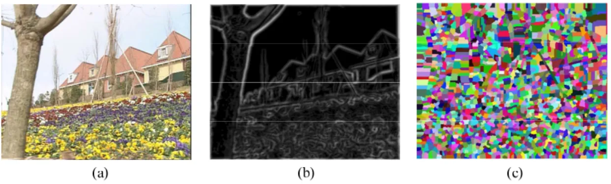
Fig. 3.4. The results of the initial segmentation process. (a) original image. (b) gradient image. (c) initial segmentation. ... 22

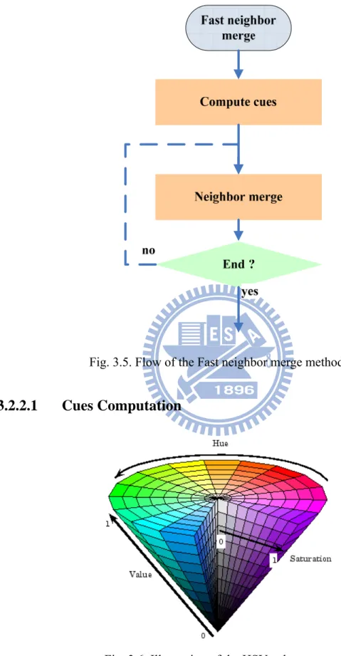
Fig. 3.5. Flow of the Fast neighbor merge method. ... 23

Fig. 3.6. Illustration of the HSV color space. ... 23

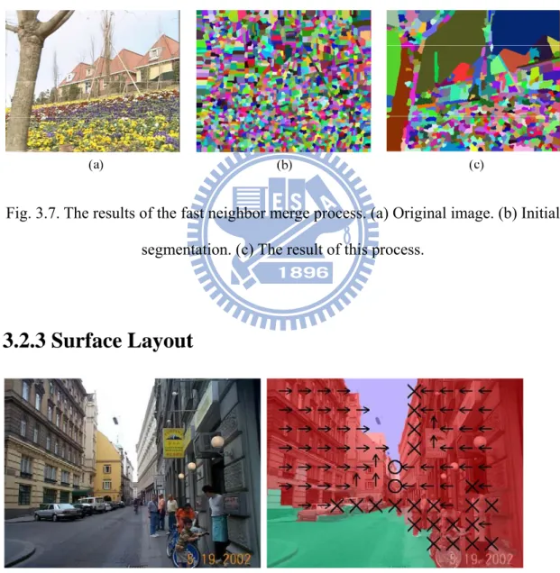
Fig. 3.7. The results of the fast neighbor merge process. (a) Original image. (b) Initial segmentation. (c) The result of this process.. ... 26

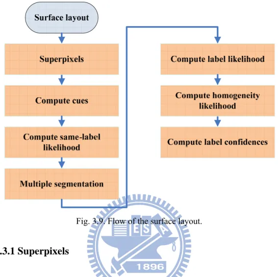
Fig. 3.8. Surface layout. On these images and elsewhere, main class labels are indicated by colors (green=support, red=vertical, blue=sky) and subclass labels are indicated by markings (left/up/right arrows for planar left/center/right, ‘O’ for porous, ‘X’ for solid)[27]. ... 26

Fig. 3.9. Flow of the surface layout.. ... 28

Fig. 3.10. The result of the confidence images for each of the surface labels.. ... 31

Fig. 3.11. Flow of the object boundary tracing method. ... 33

Fig. 3.12. The result of the initial object boundary selection.. ... 34

Fig. 3.13. A state of an object tracer in image domain.. ... 35

Fig. 3.14. The result of the object boundary tracing method. (a) Original image. (b) The result of the object boundary tracer. (c) The result of this stage. ... 36

Fig. 3.15. The result of the object segmentation. (a) Original image. (b) The result of the object boundary tracing method. (c) The result of this stage. ... 37

Fig. 3.16. Illustration of each condition for depth assignment. ... 38

Fig. 3.17. The result of depth assignment process. (a) Original image. (b) Disparity map. ... 39

Fig. 3.18. Flow of the Depth assignment process.. ... 40 

Fig. 3.19. Flow of the DIBR algorithm. ... 41

Fig. 3.20. Parallel camera configuration for virtual images warping[28]. ... 42 

Fig. 3.21. The result of DIBR algorithm. (a) Original image. (b) Disparity map. (c) Rendered left view. (d) Rendered right view. ... 43 

Fig. 4.1. Flower garden sequence ... 45 

Fig. 4.2. Hall_monitor sequence. ... 45 

x

Fig. 4.4. Outdoor0 sequence ... 46 

Fig. 4.5. Ourdoor1 sequence ... 47 

Fig. 4.6. Scenery0 sequence ... 47 

Fig. 4.7. Scenery1 sequence ... 48 

Fig. 4.8. Walking sequence. ... 48 

Fig. 4.9. Structure sequence... 49 

Fig. 4.10. Urban sequence. ... 49 

Fig. 4.11. Alley sequence. ... 50 

Fig. 4.12. 3D results of flower garden sequence with different algorithms. (a) Original image (b) Our proposed algorithm. (c) The hybrid depth cueing system. ... 51 

Fig. 4.13. 3D results of hall monitor sequence with different algorithms. (a) Original image (b) Our proposed algorithm. (c) The hybrid depth cueing system. ... 52 

Fig. 4.14. 3D results of walking sequence with different algorithms. (a) Original image (b) Our proposed algorithm. (c) The recovering major occlusion boundaries method. ... 53 

Fig. 4.15. 3D results of scenery1 with different algorithms. (a) Original image (b) Our proposed algorithm. (c) The recovering major occlusion boundaries method. ... 53 

Fig. 4.16. 3D results of alley sequence with different algorithms. (a) Original image (b) Our proposed algorithm. (c) The recovering major occlusion boundaries method. ... 54

Fig. 4.17. 3D results of outdoor0 sequence with different algorithms. (a) Original image (b) Our proposed algorithm. (c) The recovering major occlusion boundaries method. ... 54 

Fig. 4.18. 3D results of urban sequence with different algorithms. (a) Original image (b) Our proposed algorithm. (c) The recovering major occlusion boundaries method. ... 55 

Fig. 4.19. Superpixels computation with different algorithms. (a) Original image (b) Our proposed algorithm. (c) Felzenszwalb’s algorithm. ... 55 

xi List of Tables

Table 3.1. Statistics computed to represent superpixels. ... 29

Table 3.2. Statistics computed over pairs of superpixels ... 30

Table 3.2. Features of initial bounday selection ... 33

Table 3.3. Event of constraint segmentation ... 36

Table 4.1. Execution time ... 37 

1

Chapter 1. Introduction

1.1. Background

Three-dimensional (3D) video provides a dramatic enhancement in the viewing experience compared with two-dimensional (2D) video. 3D television (3D TV) applications will bring another revolution in TV’s history. The successful introduction of 3D TV to the consumer market relies on not only the technological advances but also the availability of 3D content. Due to the lack of 3D content, converting 2D video to 3D video is a promising solution to the 3D TV industrialist, especially for the traditional 2D videos

Recovering 3D information from 2D image is a basic problem in computer vision. Many depth cues can be used to extracted 3D information from 2D image, but each cue has its own advantages and disadvantages for different conditions.

Many depth cue fusion-based methods have been proposed to solve this problem. Iinuma et al. [1] use the defocus cue to evaluate the depth by a single image and the motion cue to convert the image. Cheng et al. [2] use the geometry cue and motion cue to evaluate the depth. The simple concept and low computational complexity of those methods have enabled it to be adopted real-time application. However, those methods cannot perform well for the single monocular images and the scene with complex motion.

Another approach is pattern recognition-based method. In this method, every region in the image is categorized into several classes, and every region is assigned depth according to types of the class. Battiato et al. [3] classify images into indoor,

2

outdoor with geometric elements, or outdoor without geometric elements, and use the information collected in the classification step to estimate the depth. Even through this method could generate the high quality result for single monocular image, this method cannot perform well for many types of scenes. Hoiem et al. [4] classify image as several classes. They use classified information, boundary and region, to detect the objects of image, and assign a specific depth to each object according to its classes. This method can generate high quality result for many types of scene, but its boundary extraction and object detection suffer from high computational complexity.

1.2. Motivation and Contribution

Motivated by above issues, we propose an efficient 2D to 3D conversion algorithm for monocular images in this thesis. This proposed algorithm includes image segmentation, image classification, object boundary tracing method, and 3D image generation. The image segmentation adopts the watershed method to collect the information of depth cue. Due to oversegmentation problem of watershed segmentation, we use texture and color information to merge segments. Then, we apply image classification to recover the geometry of scene in the image. In order to detect object in the image efficiently, we propose the object boundary tracing method that could quickly detect object boundary with geometry information. Finally, we apply results of object segmentation and image classification to assign depth for each object and synthesis stereo images by using the depth-based image rendering (DIBR) algorithm.

The contributions of the thesis include

1. We propose an efficient 2D to 3D conversion algorithm.

3

single image.

1.3. Thesis Organization

In Chapter 2, we introduce existing important methods for a 2D to 3D conversion system. In Chapter 3, we present the proposed object segmentation algorithm. In addition, the details of the depth assignment algorithm and the depth-based image rendering (DIBR) algorithm are illustrated. In Chapter 4, we compare the 3D results with related work, and demonstrate the execution time. Finally, we give the conclusion and future work of this thesis in Chapter 5.

4

Chapter 2. Previous Work

An important step in a 3D system is the 3D content generation. Several special cameras have been designed to generate 3D content directly. A depth-range camera [35] is an example, which is a conventional video camera with a laser element. A depth-range camera can simultaneously capture a two-dimensional RGB image and a depth map that could provide the depth information for the RGB image. This technique described above can directly generate 3D content, but the amount of traditional media data are in 2D format and demand depth information to be converted to 3D videos. Therefore, a 2D to 3D video conversion algorithm is necessary.

There are many different 2D to 3D conversion algorithm has been developed. Each algorithm has its own strength and weaknesses. Most algorithms take advantage of different depth cues to generate depth maps. In the following section, we will introduce each depth cue and many 2D to 3D systems that combine many depth cues to recovery depth information.

The structure of the chapter is as follows. In 2.1, we introduce algorithms that use a single depth cues. In 2.2, we introduce algorithms that use the depth cue fusion-based method. In 2.3, we introduce algorithms that use the pattern recognition-based method.

2.1. Various Depth Cues

Humans can straightforward determine depth from single monocular image according to experiences, which contains many monocular cues, such as defocus, texture gradients, linear perspective, contextual information. For example, objects in

5

images nearer or farther than focus are blurred, and sky in image is infinitely far away. In addition, motion parallax also is useful information to determine the depth of object. For the sequences with camera translational motion, the near objects move faster than the far objects. Depth from those cues has been developed from several years. In the Section 2.1, we introduce the principle and associated algorithms of each depth cue.

2.1.1. Depth from Camera Motion

With two images of the same scene captured from slightly different view point, the depth from camera motion can be utilized to recover the depth of an object. The relative motion between the viewing camera and the observed scene also provides an binocular disparity cue for depth perception. First, a set of corresponding points in a pair of image is found. Then, we can retrieve depth information by using the triangulation method when all camera parameters are known. If only intrinsic camera parameters are known, the depth can be recovered to a scale factor. If no camera parameters are known, the resulting depth is correct up to a projective transform. In most cases, no camera parameters are known from 2D video. Thus, we must recover camera parameters by self-calibration [5].

The typical framework in [6] using the depth from camera motion is a three-stage procedure, which is composed of feature tracking [7], structure from motion [8], and dense reconstruction. This method can extract absolute depth from 2D video with camera motion. However, in order to retrieve an accurate depth map in the dense reconstruction stage, the stereo matching algorithms [9] [10] must be used but suffer from high computational complexity. Another way to solve this problem is the realistic stereo-view synthesis (RSVS) [11]. It combines both the structure from motion and the idea of image-based rendering (IBR) [12] to achieve

6

photo-consistency without relying on dense depth estimation.

However, for still background, a scene may contain dynamic element, i.e. independent moving object. Such condition is difficult to recover camera parameters and extract depth information.

2.1.2. Individual Moving Objects

Individual moving object (IMOs) also is a depth cue in the 2D to 3D conversion system. In some cases, motion vector maps can be directly used as depth maps. This approximation holds when objects moving are with the same speed. Ideses et al. [13] extract motion vector maps from compressed 2D video, and use this information to compute depth map. However, there are many cases in which the approximation does not hold. This happens when an object without motion or not with constant speed.

Moving object segmentation also is a useful method for 2D to 3D conversion system. In this approach Kunter et al. [14] extracts the foreground objects by moving object segmentation algorithm [15], and assign depth for foreground objects. However, multiple occluding objects or objects with only little motion are difficult to detect.

2.1.3. Defocus

Cameras and eyes have limited depth of focus, so images of objects nearer or farther than focus are blurred. In other words, the amount of blur in an image is directly related to image defocus caused by the optics of the eye or camera that captures it, and can be formed a depth cue.

If a scene can be described by simply estimating which objects are in front, and which are behind those objects but are not part of the background, and what is completely in the background, we can estimate a relative depth map by taking into

7

account image blur and its relation to the focus degree in edges that compose objects. The typical algorithm of the depth from focus cue [16] uses spatial frequency measurement. When an object of an image is defocused, it will have a large

attenuation of its high spatial frequency, and when the object in a scene is focused, its high frequency component will not be attenuated and hence its sharp detail will be present as fast changes in the spatial frequency domain.

However, this method is just suitable for the close-up image, and it cannot perform well for another images.

2.1.4. Linear Perspective

Linear perspective refers to the fact that parallel lines, such as railroad tracks, appear to converge with distance, eventually reaching a vanishing point at horizon. The more the lines converge, the farther away they appear to be. A representative work is the gradient plane assignment approach proposed by Battiato et al. [3]. Their method performs well for single images containing sufficient objects of a rigid and geometric appearance. In this method, first, the edge detection is employed to locate the predominant lines in the image. Then, the intersection points of these lines are determined. The intersection with the most intersection points in the neighborhood is considered to be the vanishing point. The vanishing points are marked as the major lines close to these. The major lines close to the vanishing point are assigned a larger depth value and the density of the gradient planes is also higher.

This method is suitable for the man-made scene which contains many long and parallel lines.

8

2.1.5. Texture

Texture also offers a good 3D impression because of the two key ingredients: the distortion of individual texels and individual texture region. The latter is also called texture gradient. For example, a tiled floor with parallel lines will appear to have tilted lines in an image. The distant patches will have larger variations in the line orientations, and nearby patches will have smaller variations in line orientations. Similarly, a grass field when viewed at different distances will have different texture gradient distributions.

Texture cue is useful information to detect the depth of planar surface. If the surface is non-planar, shape-from-texture algorithms [19], [20] can be applied to reconstruct the 3D shape of object surface. However, the current algorithms cannot be applied to real-time application.

2.1.6. Relative Height

Relative height cue also offers the depth information of image. Generally, the closer objects in real world are projected into the lower part in a 2D image plane. Many photographic images, especially scenery images, have the height cue. Jung et al. [21] proposed a real-time 2D-to-3D conversion framework using the relative height cue, and many pattern recognition-based algorithms [22], [23], [27] also regard the positions of image as a cue.

2.1.7. Statistical Patterns

Statistical patterns are the elements which occur repeatedly in images. When the number or the dimension of the input data is large, the machine learning techniques

9

can be an effective way to solve the problems. In recent years, as a tool to estimate depth maps, the machine learning has been receiving increasing interest. Especially supervised learning applies training data with the ground truth to distinguish the geometry of scene, depth of scene, and stage of scene. As well as a set of representative and sufficient training data, good features and suitable classifiers are all essential ingredients for satisfactory results. More details of statistical patterns method is described in Section 2.3.

2.2 Depth Cues Fusion-based Method

In Section 2.1, we introduce many depth cues from 2D video. Each cue can recover depth information from video sequence, but it has its own advantages and disadvantages for different conditions. Several 2D to 3D systems fuse many depth cues to solve this problem. In Section 2.2, we introduce two important fusion-based methods for real-time application.

2.2.1. SANYO 2D to 3D Conversion Adaptive Algorithm

The 2D-to-3D image conversion technique using the “Modified Time Difference method” (MTD) [24] had been developed in 1995. To convert from 2D video into 3D video, the MTD select another frame to be a stereo-pair according for each frame. The selection criterion is based on the object motion in the successive frames.

The 2D images, having the objects with simple horizontal motion, can be converted into 3D images by the MTD well. However, it is not good for converting from the still images or the images that have the objects with complicated motions. So the technique converting from these 2D images into 3D images is required.

10

subject. The CID allows to converting from single monocular 2D images into 3D images, and the CID uses the defocus cue to extract depth information. They compute contrast, sharpness and chrominance of the image to extract the defocus cue. The sharpness means the high frequency component of the image luminance. The contrast means the middle frequency component of the image luminance. The chrominance means the hue and tint of the image color. The 3D images are generated by computing the depth cue of each separated area of the input 2D. In the CID, first the adjacent areas, which have close color, are grouped according to the chrominance values. Then the distance from the camera to the objects is computed, and it should be inversely proportional to the contrast and sharpness values. The close-up images can be converted into 3D images by the CID, but it is not good for converting from other types of images.

These techniques have been implemented into a single-chip LSI for the automatic and real-time 2D-to-3D image conversion, and can output 3D image according to various 3D displays from various input images, like NTSC, PAL, HDTV, and VGA.

2.2.2. Hybrid Depth Cueing System

The hybrid depth cueing system [2] had been developed in 2009. The depth generation method consists of the depth from motion parallax (DMP) and the depth from geometrical perspective (DGP). And the depth fusion-based method is used to combine DMP and DGP according to adapted weighting factors. Finally, the DIBR renders multiple views with various view angles for 3D displays.

The DMP module is the central core of the system. The DMP consists of the following two processes.

11

consecutive video frames. 4-parameter global motion estimation [36] is used between all the continuous frame pairs. Then, the most suitable frame in frame buffer is selected and is warped to form parallel view configuration with the current frame. The other is the disparity estimation process that generates the depth map according to the image pair. Block-based motion estimation is used between selected image pair. Disparity map is retrieved when static scene with camera translational motion. When the scene happen individual moving objects, motion vector is used as a depth cues.

The visual effect is that moving objects will pop-up and catch more attention. The depth was estimated by 2 2

y x MV

MV +

In order to adapt this technique to the automatic and real-time 2D-to-3D image conversion, they had improved the DMP to handle more complex motion cases than the MTD. But the DMP could not perform well for the video that has changing focal length or dynamic scene.

When the depth information cannot derive from the motion information, monocular depth cue become an important issue in depth generation. Depth from geometrical perspective (DGP) classifies the scene into multiple modes by scene line structure detection. The major types are horizontal lines and vanishing lines. Fig. 2.1 shows multiple scene modes that DGP classifies.

Fig. 2.1. Multiple scene modes using depth from geometry [2]

But the DGP is only suitable for background region in the image. If the DMP cannot work, the DGP is not good enough to generate good visual effect.

12

Finally, fusion-based method is used to combine both depth maps. The weighting factor is adjusted that depending on the camera motion analysis module. When camera is panning depth can be retrieved from motion parallax efficiently. Weight for DMP will adjust to larger.

2.3 Pattern Recognition-based Method

Even through the depth cues fusion-based methods mentioned in Section 2.2 could be used for real-time application, they still have problem in depth from monocular images. Pattern recognition-based methods are more suitable to solve this problem. Nedovic et al. [18] categorize the input image into various types and limited number of stages in each type to simplify the problem. But this method only computes the background of depth map. Saxena et al. [22] [23] also presented a method to learn absolute depth from single images based on low-level features, but this method only suitable for outdoor scene. In the following, we introduce two methods. The first method is proposed by Battiato et al. [3]. It is suitable for real-time application, but it cannot assign depth for all objects in the image. The second method is proposed by Hoiem et al. [4]. This method is suitable for most cases of image, but it has high computational complexity.

2.3.1 Depth-Map Generation by Image Classification

This algorithm [3] is performed on a single color image, and does not need any prior knowledge about image content. It is also claimed to be fully unsupervised and suitable for real-time applications. In this algorithm, two intermediate depth maps, the qualitative depth map and the geometric depth map, are constructed.. In the end, these two depth maps are combined together to generate the final depth map.

13

Fig. 2.2. block diagram of algorithm [3]

Fig. 2.2 shows the block diagram of algorithm [3]. At first, mean shift segmentation algorithm is used to partition image. Then, in order to generate qualitative depth map, color-based rules are used to identify six semantic regions: Sky, Farthest Mountain, Far Mountain, Near Mountain, Land and Other. Each semantic region is assigned a depth level, which corresponds to a certain gray level following the trend: Gray of Sky < Gray of Furthest Mountain < Gray of Far Mountain < Gray of Near Mountain < Gray of Land < Gray of Other.

In third stage, The qualitative depth map is then sampled column-wise. Each column is represented by a label sequence, which is labeled from top to down, and each region present in the column. After all the sequences in the image have been generated, they are plugged into a counting process to obtain the number of accepted sequences. Finally, they use the number of accepted sequences to classify the image

14

into three categories: outdoor, outdoor with geometric appearance and indoor.

They also apply linear perspective cue. Different vanishing line detection strategies are applied according to the category to which the image belongs. For Outdoor scenes, the vanishing point is put in the center region of the image and a set of vanishing lines passing through the vanishing points are generated. For the categories Indoor and Outdoor with geometric appearance, a more complex technique is applied. Edge detection and line detection are conducted to determine the main straight lines. The vanishing point is chosen as the intersection point with the most intersections around it while the vanishing lines are the predominant lines passing close to the vanishing point.

After the vanish point detection, taking the position of the vanishing point into account, a set of horizontal or vertical gradient planes is assigned to each neighboring pair of vanishing lines. The resultant image is termed the geometric depth map. Then, the qualitative depth map is checked for consistency. False classified semantic regions are detected and corrected.

Finally, the final depth map of indoor category image is just the geometric depth map. For outdoor without geometric appearance, the final depth map is qualitative depth map. For the image category of outdoor with geometric appearance, the final depth of pixel is assigned the depth value in the geometric depth map for all cases, except when it is a sky, it then adopts the depth value in the qualitative depth map.

The natural images and man-made structure can be converted into 3D images by this method. But it is not good for converting images that contain non-definition object.

15

2.3.2 Recovering Major Occlusion Boundaries

Single-view 3D reconstruction is a popular research in computer vision. Even though they are not ready for real-time application due to high computation complexity, their qualities are good enough to use. An algorithm of Hoiem [4] et al. describes the property of the regions and boundaries in the image, and the 3D surfaces of the scene using learned model. Their representation includes a wide variety of cues: color, position, and alignment of region; strength and length of boundaries; 3D surface orientation estimates; and depth estimate. In a conditional random field (CRF) model, they also encode gestalt cues, such as continuity and closure, and enforce consistency between our surface and boundary labels.

To provide an initial conservative hypothesis of the occlusion boundaries, they apply the watershed segmentation algorithm to the soft boundary map provided by the pB algorithm of Martin et al. [26]. This segmentation produces thousands of regions that preserves nearly all true boundaries. In training, they assign ground truth to this initial hypothesis. Given a new image, their task is to group the small initial regions into objects, and assign figure/ground labels to the remaining boundaries.

To get a final solution, they could simply compute cues over each region and boundary, and perform a single segmentation and labeling step. However, the small regions from the initial over-segmentation do not allow the more complicated cues, such as depth, to be reliable. Furthermore, global reasoning with these initial boundaries is ineffective because most of them are spurious texture edges.

Their solution is to gradually evolve their segmentation by iteratively computing cues over the current segmentation and using them with our learned models to merge regions that are likely to be part of the same object. In each iteration, the growing

16

regions provide better spatial support for complex cues and global reasoning. And better spatial support can improve their ability to determine whether remaining boundaries are likely to be caused by occlusions. See Fig. 2.3 for an illustration. Each iteration consists of three steps based on the image and the current segmentation: 1) compute cues; 2) assign confidences to boundaries and regions; and 3) remove weak boundaries, forming larger regions for the next segmentation.

Fig 2.3. Illustration of the recovering major occlusion boundaries algorithm. [4]

In most cases, 2D images can be converted into 3D images by this method, but it is not good for real-time application. In their Matlab implementation, this algorithm takes about 4 minutes for a 600x800 image on a 64-bit 2.6GHz Athalon running Linux.

17

3. 3D Image Construction from 2D Image

3.1. Algorithm Overview

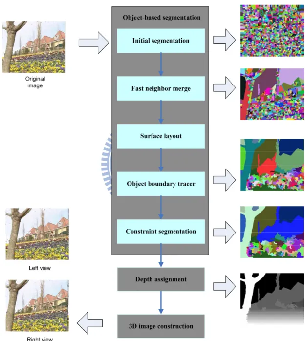
Fig. 3.1. Flow of the proposed 2D to 3D conversion system.

In this chapter, we propose a fast and effective 2D to 3D conversion algorithm with the pattern recognition-based method. Fig. 3.1 illustrates the flow of the 2D to 3D

18

conversion system, which consists of three main processes: object-based segmentation, depth assignment, and 3D image construction.

For the object-based segmentation, we first use the watershed segmentation algorithm to compute the initial segmentation. Even though the watershed segmentation can preserve object boundary well, it has problems of over segmentation and sensitivity to noise. Due to oversegmentation problem that produces from watershed segmentation, fast neighbor merge process is used to solve this. At the third step, we use the surface layout algorithm [10] to provide the geometric information for object detection. At the fourth step, inspired by the recovering occlusion boundaries method in [4], we propose the object boundary tracing method to detect object efficiently. After the object boundary tracing method, there are still some incomplete object segments. Thus, we perform the constraint segmentation, which builds some conditions to merge segments. After the constraint segmentation process, the object-based segmentation is done.

Finally, we assign the depths to the objects, and use the DIBR algorithm [28] to generate the images for left and right eyes.

3.2. Object-based Segmentation

3.2.1 Initial Segmentation

In the proposed 2D to 3D conversion system, a precise estimation of object boundary is important. Thus a proper choice of image segmentation algorithm is also important in our case. We adopt watershed image segmentation from all existing image segmentation algorithms for the two reasons: (1) it can preserve edge in the object boundary [37]; (2) it is suitable for fast application [38].

19

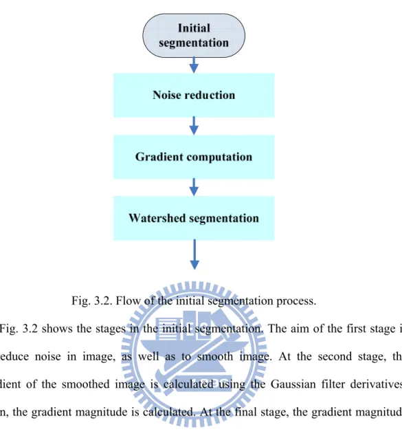
Fig. 3.2. Flow of the initial segmentation process.

Fig. 3.2 shows the stages in the initial segmentation. The aim of the first stage is to reduce noise in image, as well as to smooth image. At the second stage, the gradient of the smoothed image is calculated using the Gaussian filter derivatives. Then, the gradient magnitude is calculated. At the final stage, the gradient magnitude is thresholded appropriately and watershed transform produces an initial image partition.

3.2.1.1. Noise Reduction and Gradient Computation

At the first stage of the initial segmentation, we use a Gaussian filter to smooth the image slightly before computing image gradient. In order to compensate for digitization artifacts, we always use a Gaussian with the σ of 0.8. It does not produce any visible change to the image but help remove artifacts.

At the second stage of the initial segmentation, the gradient field of the smoothed image is computed. The derivitave of Gaussian with the σ of 1.0 and the support size

20

of 9x9 is used to compute the gradient of the smoothed image L and L . Finally, the gradient magnitude image G(I) is calculated by following formula

| | (3.1)

3.2.1.2. Watersheds Segmentation

In this stage, an initial image partitioned into primitive regions is obtained using the image gradient magnitude and watershed algorithm. Watershed segmentation is a popular and well known algorithm that extracts regions as catchment basins based on the concept of topography. The gradient image of the input image is used as the topographic surface in which the gradient value represents the altitude. The segmentation of an image finds the watershed line on the gradient image and thus separates each region. In the following, we briefly describe the parallel watershed transform proposed by Giovani et al. [29].

The algorithm is composed of the four major steps, finding the lowest neighbor of each pixel (i.e. direct path of steepest descent), finding the nearest border of internal pixels of plateaus, propagating uniformly from the borders, and minima labeling by maximal neighbor address and pixel labeling by flooding from minima. Fig. 3.3 presents a parallel watershed transform, where I is the input image, and lab is the output labeled image that is also used for storing addresses. The statement for all denotes that every iteration can be processed in parallel.

// First Step 1: PLATEAU ← +∞ 2: for all p D do

3: if q N(p) : I(q) < I(p) and I(q) = min q’ N(p)I(q’) then 4: lab(p) ← -q 5: else 6: lab(p) ← PLATEAU 7: end if 8: end for // Second step

21 10: lab’ ← lab

11: for all p D : lab(p) = PLATEAU do

12: if q N(p) : lab(q) <= 0 and I(q) = I(p) then 13: lab’(p) ← -q 14: end if 15: end for 16: lab ← lab’ 17: end while // Third step 18: basins ← 1 19: for p D do

20: if lab(p) = PLATEAU then 21: lab(p) ← basins 22: basins ← basins + 1 23: QUEUEPUSH(p)

24: while QUEUEEMPTY( ) = False do 25: q ← QUEUEPOP( )

26: for u N(q) do

27: if lab(u) = PLATEAU then 28: lab(u) ← lab(p) 29: QUEUEPUSH(u) 30: end if 31: end for 32: end while 33: end if 34: end for // Fourth step 35: for p D do 36: if lab(p) <= 0 then 37: q ← p 38: while lab(q) <= 0 do 39: q ← -lab(q) 40: end while 41: u ← p 42: while u q do 43: v ← u 44: u ← -lab(u) 45: lab(v) ← lab(q) 46: end while 47: end if 48: end for

Fig. 3.3. Pseudo code of the parallel watershed transform [29].

The watershed transform is applied to the thresholded gradient magnitude image

GT, where the pixels of G having value smaller than a given threshold T are set to zero. That is

,

0, (3.2)

22

Due to thresholding, many of the regional minima of G located in homogeneous region are replaced by fewer zero-valued regional minima in GT. It could slightly limit the size of the initial image partition is to prevent over-segmentation in homogeneous region. Fig. 3.4 shows the results of the initial segmentation process.

Fig. 3.4. The results of the initial segmentation process. (a) original image. (b) gradient image. (c) initial segmentation.

3.2.2 Fast neighbor merge

In addition to the above over-segmentation reduction method, there still remain neighboring regions that be merged into a meaningful segmentation, Fast neighbor merge method is used to guarantee that segments are large enough.

Fig. 3.5 shows the stages of the Fast neighbor merge method. The aim of the first stage is the cue computation. Those cues are color and texture. At the second stage, we use those cues to decide whether the segment could be merged or not.

23

Fig. 3.5. Flow of the Fast neighbor merge method.

3.2.2.1 Cues Computation

Fig. 3.6. Illustration of the HSV color space.

24

important. Thus a proper choice of color space is important in our case. In our case we consider the Hue-Saturation-Value (HSV) color space [30], because it is very similar to the human perception of colors. Fig. 3.6 is Illustration of the HSV color space. Conceptually, the HSV color space is a cone. Viewed from the circular side of the cone, the hues are represented by the angle of each color in the cone relative to the 0° line, which is traditionally assigned to be red. The saturation is represented as the distance from the center of the circle. Highly saturated colors are on the outer edge of the cone, whereas gray tones (which have no saturation) are at the center. The value is determined by the colors vertical position in the cone. At the pointy end of the cone, there is no brightness, so all colors are black. At the fat end of the cone are the brightest colors.

Color transformation from RGB to HSV color space is done by the following , , (3.3) , , (3.4) 0°, max 60° ⁄ 0°, max 60° ⁄ 360°, max 60° ⁄ 120°, max 60° ⁄ 240°, max (3.5) 0, max 0 ⁄ ⁄ , (3.6) (3.7) Color difference _, between two points pi[hi, si, vi], pj[hj, sj, vj] in the HSV space is given by the formula[31]

, 1 1 √5⁄ cos cos sin

25

For every segment, we compute average RGB value, and transform average RGB value to HSV color space. Then, we compute color difference for every neighboring segment.

Another cue is texture. Similarly to color, texture provides a cue for the geometric class of a segment through its relationship to materials and objects in the world.

To represent texture, we apply a subset of the filter bank designed by Leung and Malik [32]. We generated the filters with the following parameters: 19x19pixel support, the scale of √2 for oriented and blob filters, and 6 orientations. For the filter bank, there are 6 edges, 6 bars, 1 Gaussian, and 2 Laplacian of Gaussian filters.

We compute the histogram (over pixels within a segment) of maximum responses. Then, we compute the symmetrized Kullback-Leibler divergence , for every neighboring segment.

Finally, we compute the cost function E which is combine color and texture information for every neighbor segments by the formula,

, , , (3.9) where , are the weighting factors to control the amount of each energy.

3.2.2.2 Neighbor Merge

In this stage, we use connected components for segment merge. Connected components are the simplest method of image segmentation. During the Connected components process, if their cost E is smaller than some threshold values, two neighboring segments are merged. The key parameter in the connected components process is the threshold T. We use the following iterative method to determine the threshold T:

26

2. If the cost of neighboring segment is smaller than the threshold T, we will merge neighboring segment.

3. Turn up the threshold T.

4. Go back to step 2, and replace the threshold T. Keep repeating until the number of segment is smaller than a constant NS, 1000.

Fig. 3.7 shows the results of the fast neighbor merge process.

Fig. 3.7. The results of the fast neighbor merge process. (a) Original image. (b) Initial segmentation. (c) The result of this process.

3.2.3 Surface Layout

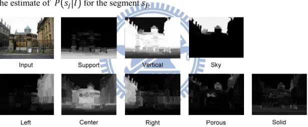
Fig. 3.8. Surface layout [27]. On these images and elsewhere, main class labels are indicated by colors (green=support, red=vertical, blue=sky) and subclass labels are indicated by markings (left/up/right arrows for planar left/center/right, ‘O’ for porous, ‘X’ for solid).

27

Surface layout proposed in [27] can label the image into geometry classes, which coarsely describe the 3D scene orientation of each image region as shown in Fig. 3.8. Every region in the image is categorized into one of three main classes: “support”, “vertical”, and “sky”. Support surface are parallel to the ground and could potentially support a solid object. Vertical surfaces are solid surfaces that are too steep to support an object. The sky is the image region corresponding to the open air and clouds. Vertical class is further categorized into one of five subclasses: “left”, “center”, “right”, “porous”, and “solid”. Planar surfaces facing to the “left”, “center” or “right” of the viewer, and non-planar surface that are either “porous” or “solid”.

We believe that surface layout representation is useful information for us to detect object in the image. Fig. 3.9 shows the stages of the surface layout. At first, image is partitioned to many superpixels, and we compute cues for each superpixels. In order to have better result, multiple segmentation is used, so same-label likelihood is computed to be cost information for merge segment. After multiple segmentation, homogeneity likelihood is computed for each segment, and it is used to determine that segment is homogeneity or not. Label likelihood is also computed for each segment and superpixel to determine that segment belongs to which category. Finally, Bayes theorem applies label likelihood and homogeneity likelihood to compute the label confidence for each superpixel. We will briefly describe the stages in following section.

28

Fig. 3.9. Flow of the surface layout.

3.2.3.1 Superpixels

The use of superpixels improves the computational efficiency of our algorithm, and allows complex statistics to be computed for enhancing our knowledge of the image structure. Different from original algorithm in [34], we adopt our initial segmentation as superpixels.

3.2.3.2 Cues computation

To determine which orientation is most likely, we need to use all of the available cues: location, color, texture, perspective. In Table 3.1, we list the set of statistics used for classification.

29

Table 3.1. Statistics computed to represent superpixels [27] Surface Cues

Location

L1. Location: normalized x and y, mean

L2. Location: normalized x and y, 10th and 90th pctl

L3. Location: normalized y wrt estimated horizon, 10th, 90th pctl

L4. Location: whether segment is above, below, or straddles estimated horizon L5. Shape: number of superpixels in segment

L6. Shape: normalized area in image

Color

C1. RGB values: mean

C2. HSV values: C1 in HSV space C3. Hue: histogram (5 bins) C4. Saturation: histogram (3 bins)

Texture

T1. LM filters: mean absolute response (15 filters) T2. LM filters: histogram of maximum responses (15 bins)

Perspective

P1. Long Lines: (number of line pixels)/sqrt(area) P2. Long Lines: percent of nearly parallel pairs of lines P3. Line Intersections: histogram over 8 orientations, entropy P4. Line Intersections: percent right of image center

P5. Line Intersections: percent above image center

P6. Line Intersections: percent far from image center at 8 orientations P7. Line Intersections: percent very far from image center at 8 orientations P8. Vanishing Points: (num line pixels with vertical VP membership)/sqrt(area) P9. Vanishing Points: (num line pixels with horizontal VP membership)/sqrt(area) P10. Vanishing Points: percent of total line pixels with vertical VP membership P11. Vanishing Points: x-pos of horizontal VP - segment center (0 if none) P12. Vanishing Points: y-pos of highest/lowest vertical VP wrt segment center P13. Vanishing Points: segment bounds wrt horizontal VP

P14. Gradient: x, y center of mass of gradient magnitude wrt segment center

3.2.3.3 Same-label Likelihoods

30

outputs an estimate of for the adjacent superpixels i and j and image data I. Here and are the superpixel label. The same-label classifier is based on cue set L1, L6, C1-C4, and T1-T2 in Table 3.1. In Table 3.2 we list the set of statistics used for computing same-label likelihoods.

Table 3.2. Statistics computed over pairs of superpixels Boundary cues

Location

the absolute differences of the pixel location values x and y

Color

C1. the absolute differences of the mean RGB C2. the absolute differences of the mean HSV

C3. the symmetrized Kullback-Leibler divergence of the hue C4. the symmetrized Kullback-Leibler divergence of the saturation

Texture

T1. the absolute differences of the mean LM filter response

T2. he symmetrized Kullback-Leibler divergence of texture histogram

Shape

S1. the ratio of the area

S2. the fraction of the boundary length divided by the perimeter of the smaller superpixel S3.the straightness of the boundary

3.2.3.4 Multiple Segmentations

The increased spatial support of superpixels provides much better classification performance than for pixels. Large regions are required to effectively use the more complex cues. We need to compute multiple segmentations and then use the increased spatial support provided by each segment to better evaluate its quality. This method is based on pairwise same-label likelihoods. A diverse sampling of segmentations is produced by varying the number of segments nsand using a random initialization.

31

3.2.3.5 Label Likelihood Computation

The label classifier is used to distinguish among the main classes and the subclasses, and it is based on all of the listed cues. The label classifier output the estimate of , for the segment .

3.2.3.6 Homogeneity Likelihood Computation

The homogeneity classifier is used to determine whether a segment has a single or is mixed, and it is based on all of the listed cues. The homogeneity classifier output the estimate of for the segment .

Fig. 3.10. The result of the confidence images for each of the surface labels.

3.2.3.7 Label Confidences Computation

In final stage, we compute label confidences for each superpixel, and use following formula:

| ∑ , (3.10) Fig. 3.10 shows the result of the confidence images for each of the surface labels.

32

3.2.4 Object Boundary Tracing Method

There are many features that could be used to detect the object boundary, and we describe below. Adjacent regions have different colors or textures, or are misaligned; long and smooth boundaries with strong color or texture gradients; two adjacent regions have different 3D surface characteristics.

Until now, we extract many features that could be used to detect object, but how to use them efficiently? Local method is difficult to distinguish the correct boundary, while global method has high computational complexity due to much iteration. Therefore, we propose an object boundary tracing method to solve this problem. Fig. 3.11 shows the stages of the object boundary tracing method. The aim of the first stage is the initial boundary selection, and obvious object boundaries are labeled using the rule-based method. At the second stage, the rest of object boundaries are traced from the initial boundaries. At the third stage, segments without object boundary are merged

33

Fig. 3.11. Flow of the object boundary tracing method.

3.2.4.1 Initial Boundary Selection

There are many features that we compute before and could be used to detect object boundary. As the situation is different, we should choose different features, so we categorize every object boundary in the image into one of three classes: “gnd-vrt”, “sky-vrt”, and “vrt-vrt” as in Table 3.3. For different class, we use a specific feature to determine its initial boundaries.

Table 3.3. Features of initial boundary selection.

Class features

for all classes boundary smoothness

34

for “gnd-vrt” class only main label likelihood

for “sky-vrt” class only main label likelihood

for “vrt-vrt” class only sub-label likelihood

if event vrt-gnd-vrt

We use a set of rule to determine the initial boundary. For example given the “sky-vrt” class of the boundary it belongs to initial object boundary if the following condition is satisfied:

z 1 0.5

0.3 0.3

The denotes the same-label likelihood and the

denotes the sky label confidence. Similar conditions have been used in order to detect the other classes of object boundary, more detail formula that we show in appendix. Fig 3.12 shows the result of the initial object boundary selection. The red fragments in the image are selected initial object boundaries.

Fig 3.12. The result of the initial object boundary selection.

3.2.4.2 Object Boundary Tracer

The object boundary tracer of a boundary start from an initial object boundary and selects a next object boundary. The selected object boundary should have high edge value, and high label likelihood difference, and the property of the class of object boundary, and the boundary orientation should not change rapidly. This process

35

repeats until reaching to the border of image or the object boundary that already be labeled. Fig. 3.13 shows a state of an object tracer in image domain.

x y

Current boundary position

Next boundary position

Fig 3.13. A state of an object tracer in image domain

We develop an energy function for the object boundary tracer. The energy function is modeled by three constraints. The first is the boundary tracing constraint to trace strong boundary. The second is the different label constraint to separate different object. The third is the same label constraint to penalize significant surface label changes in an object.

The following equation describe above three constraints. Constraint 1: boundary tracing constraint:

, 1 , (3.11) Constraint 2: different label constraint:

, , (3.12)

Constraint 3: same label constraint:

, , , (3.13)

36

and are the superpixel label. Then, the object boundary tracing problem can be formulated as follows.

, , , , (3.14)

where , , are the weighting factors to control the amount of each energy.

Then, we need to find the solution by solving the problem. Because we want to save computation, we just use local method to minimize the cost function. Fig 3.14 shows the result of the object boundary tracing method. In Fig. 3.14(b), the white line is the selected object boundary.

Fig 3.14. The result of the object boundary tracing method. (a) Original image. (b) The result of the object boundary tracer. (c) The result of this stage.

3.2.5 Constraint Segmentation

Table 3.4. Events of constraint segmentation Event 1: the color of the segment is similar to the other.

Event 2: the label confidence of the segment is similar to the other. Event 3: the shape of the segment is similar to the other.

Event 4: the y axis position of the segment is similar to the other. Event 5: the segment is inside of the other segment.

Event 6: the segment is small enough.

37

complete objects. There are many events that could help us merge those segments. Table 3.4 lists theses event that we use. In order to merge them, we construct several rules. We merge the segments, if the following conditions are satisfied.

Condition 1: 1 2

Condition 2: 1 2 6

Condition 3: 2 3 4

Condition 4: 2 5

We seriatim check conditions, and merge the segments, after the constraint segmentation process, the object segmentation is done. Fig. 3.15 shows the result of the object segmentation.

Fig 3.15. The result of the object segmentation. (a) Original image. (b) The result of the object boundary tracing method. (c) The result of this stage.

3.3 Depth Assignment

After the object segmentation stage, we assign the depth to the objects. Our model in the 3-dimensional space consists of a ground plane and objects are orthogonal to the ground and sky. In order to construct 3D image for binocular vision, the depth assignment process output the disparity map , in the range of 0-255, disparity map is encoded the depth information. In our image coordinate system, the origin is

38

located at the most left-up corner, and the x-axis toward right, and the y-axis toward down.

Fig. 3.16. illustration of each condition for depth assignment

We assign different depth for segment according to their conditions. Fig. 3.16 shows those conditions that we consider. Fig 3.18 shows the stages of the depth assignment process. At first, for each region, we fit a set of line segments to the ground-vertical boundary by using the Hough transform [33]. Those line segments are used to determine that the vertical labeled vertical segments are planar or not. If vertical labeled segments contain the line segment, it is planar. Otherwise vertical labeled segment is non-planar. Then we begin to assign depth to each segment.

For the ground labeled segment, we compute disparity by the formula:

39

where H is the height of the image, and hpos is the position of the horizontal line in the image that is computed by vanish point or the highest position of ground labeled pixel.

For the vertical labeled segment that is connected with ground labeled segment, if the ground-vertical boundary is a line, we use following formula:

, ⁄ 255.0⁄ (3.16) ⁄ (3.17) , , (3.18)

where , is the linear equation of the line segment.

For the vertical labeled segment, if the segment is planar, we also use formula (3.14) and (3.15). However the linear equation is different. The slope of the linear equation is decided by sub-class, and the line through the point that is the lowest y-axis position of the segment in the image.

If the segment is non-planar, we use following formula,

, ⁄ 255.0⁄ , (3.19)

where is the lowest y-axis position of the segment in the image.

After depth assignment process, the disparity map is computed. Fig. 3.17 shows the result of depth assignment process.

40

Fig. 3.17 The result of depth assignment process. (a) Original image. (b) Disparity map.

41

3.4 3D Image Construction for Binocular vision

Fig. 3.19 Flow of the DIBR algorithm.

After we have the disparity map, we can generate left and right eye images by the depth-based image rendering (DIBR) algorithm [28].

Fig. 3.19 shows the stages of the DIBR algorithm. The concept of DIBR on the parallel camera configuration as shown in Fig. 3.20 . In this configuration, an object O is observed at original center view Vc, and virtual left-eye view Vl. This object is also projected to Xc, Xr, and Xl in the image planes respectively. The relationship of the projected position among views is

2

⁄ ⁄ ⁄2 ⁄ , (3.20) where Z is the depth of object from the view plane f is the focal length and b is the baseline of Vr and Vl. Because we can’t know the camera parameter in original 2-dimensional video, we simplify the formula

2

42

where d is the disparity that compute from Section 3.3 and s is the scale factor that could be adjusted by user.

Fig. 3.20. Parallel camera configuration for virtual images warping [28]

If disparity map is given, we can render the virtual left-eye and right-eye view images using the center view image. This rendering process is generally called 3D warping. However, the warped virtual images incur many holes, which may be seen by the right eye or left eye but occluded in the center view. To recover the holes, the hole-filling method is added after the 3D warping process as shown in Fig. 3.19 . But it suffers from serious texture distortion since the large holes cannot be recovered well. The depth smoothing method is adopted before the 3D warping process. The aim of the depth smoothing is to reduce the size of holes. In the depth smoothing stage, directional Gaussian filter is used to reduce the geometric distortion, and apply filter only on the hole-region. Fig. 3.21 shows the result of DIBR algorithm.

43

Fig. 3.21. The result of DIBR algorithm. (a) Original image. (b) Disparity map. (c) Rendered left view. (d) Rendered right view.

44

4. Experimental Results and Analysis

4.1. Introduction

In this chapter, we show the experimental results of the proposed 2D to 3D conversion system on test images. The experimental results contain 3D result and execution time. The test images are used from the Internet. In addition to the 3D result of our proposed system, we included the 3D result of the hybrid depth cueing system [2] and the recovering major occlusion boundaries method [4] for comparison. The source codes of recovering major occlusion boundaries method for comparison is provided from [4].

4.2. 3D Results

4.2.1. Our 3D Results

The proposed method has been tested using different types of scenarios. The generated disparity maps, rendered left and right view images and anaglyph images are showed from Fig 4.1 to Fig 4.11 for evaluation. Sequences in the Fig 4.1 and Fig 4.2 are standard MPEG-4 video test sequences. Other sequences are selected from the databases of [4].

In the test image “flower garden” as shown in Fig. 4.1. It is tested for outdoor scene. There are four major parts that should be partitioned. They are sky, ground, tree, and building. The result of disparity map shows that depth of objects is correct.

45

There are five major parts that should be partitioned. They are ground, ceil, left wall, right wall, and man. Even through objects in the image are not detected well, the order of depth is correct. The result also shows that out system can handle planar surface.

Fig. 4.1. Flower garden sequence.

Hall_monitor sequence Disparity map Anaglyph Left view Right view

46

Fig. 4.3. Building.

Fig. 4.4. Outdoor0 sequence.

Fig . 4.3 and Fig. 4.4 are tested for outdoor scene with geometry. In Fig. 4.3, the major part in the image is building, and result of depth is correct. The chair in the image is not detected well, because the geometry of result for the chair is ground label. In Fig. 4.4, the order of depth is correct, but the woman in the image right side is

47

merged with building. The mistake is caused by object boundary tracer.

Fig. 4.5. Ourdoor1 sequence.

Fig. 4.6. Scenery0 sequence.

Fig. 4.5 and fig. 4.6 are tested for nature outdoor scene. The result of Fig. 4.5 is good. In the fig 4.6, many birds in the image are not detected. It is because the

48

geometry of result is wrong.

scenery1

Disparity

map Anaglyph

Left view

Right view

Fig. 4.7. Scenery1 sequence.

49 structure Disparity map Anaglyph Left view Right view

Fig. 4.9. Structure sequence.

scenery1 (a)

Disparity map Left view Right view

(b)

Disparity map Left view Right view

(c)

50

Fig. 4.11. Alley sequence.

In Fig 4.7, Fig 4.8, and Fig 4.10 are tested for nature outdoor scene with people. Results show that the people in the image are detected well, and even people wear camouflage in the woods.

Fig 4.9 and Fig 4.11 are tested for man-made scene. The result of fig 4.9 is good. Even through the order of depth in the fig 4.11 is correct, but woman in the image right side is merged with tree, ground, and statue. This makes it impossible to

51

4.2.2.3D Result Comparison between Different Algorithms

In this section, we compare our method with the hybrid depth cueing system and the recovering major occlusion boundaries method.

The 3D result of the hybrid depth cueing system is showed from Fig. 4.12 to Fig. 4.13. In flower garden sequence, Fig. 4.12(c) show the DMP, DGP, fused disparity map, left view and right view, where DMP is depth from motion, DGP is depth from single image. Compare with our method in Fig. 4.12(b), our disparity map is better, because our depth of the building in the image is more accurate. If we only consider the condition that is depth from single image, our method computes the depth of objects is more accurate. Because the DGP can’t compute the depth of objects, it just can compute the depth of the background. In the hall monitor sequence, the result of the hybrid depth cueing system is better for the depth of background, but our method just use single image to compute the depth of the scene. If their result misses motion information, they could not compute the depth of man.

Fig. 4.12. 3D results of flower garden sequence with different algorithms. (a) Original image (b) Our proposed algorithm. (c) The hybrid depth cueing system.