建立蛋白質資料庫與知識庫

全文

(1)國立交通大學 ၅૩࣫Ꮠ‫!ء‬ 碩士論文建立蛋白質資料庫與知識庫. Construction and Implementation of Protein Database and Knowledge Base. 研究生：顧世彥指導教授：胡毓志楊維邦. 教授教授. 中華民國九十四年六月.

(2) 建立蛋白質資料庫與知識庫 Construction and Implementation of Protein Database and Knowledge Base. 研究生：顧世彥. Student：Shih-Yen Ku. 指導教授：胡毓志. Advisor：Yuh-Jyh Hu. 楊維邦. Wei-Pong Yang. 國立交通大學資訊科學系碩士論文 A Thesis Submitted to Department of Computer and Information Science College of Electrical Engineering and Computer Science National Chiao Tung University in partial Fulfillment of the Requirements for the Degree of Master in Computer and Information Science June 2005 Hsinchu, Taiwan, Republic of China. 中華民國九十四年六月.

(3) 建立蛋白質資料庫與知識庫. 研究生：顧世彥. 指導教授：胡毓志博士楊維邦博士. 國立交通大學資訊科學研究所. 摘要. 本篇論文最主要的是提供一個範例,這個範例是建構我們自己特有的蛋白質資料庫,並且發展我們自己一套資料採礦的方法去建構出我們自己特有的蛋白質知識庫.在本篇論文裡,我們利用我們發展的一套組合式方法(SUM-K)去找出蛋白質的基本結構並將其轉換成一套足以代表蛋白質結構特性的字母系統.利用這樣具有結構特性的字母系統,我們可以下去進行結構相似度分析,並且搭配利用 1D 排比的工具,如此可以快速的比對出結構相似度高的蛋白質.我們也針對 SCOP 蛋白質資料做了一系列的實驗,實驗驗證了我們字母系統優於其他字母統且我們所提出的方法(SUM-K)不但可行而且可以找到最能代表蛋白質結構的結構字母轉換系統.我們也將轉好的字母系統存到了知識庫中,另外我們也提供了網路介面給使用者來分析自己有興趣的蛋白質.. i.

(4) Construction and Implementation of Protein Database and Knowledge Base Student：Shih-Yen Ku. Advisor：Dr. Yuh-Jyh Hu Dr. Wei-Pong Yang. Institute of Computer and Information Science National Chiao Tung University Hsinchu, Taiwan, 300, Republic of China Abstarct. The purpose of this thesis is providing an example of constructing our protein database and developing the combinatorial data mining approach to construct our protein knowledge base. In this thesis, the combinatorial approach (SUM-K) found the basic building blocks of protein structure and defined the structure alphabet (SA). The structure alphabet can represent the structural information of protein and transform the original sequences into sequences of structure alphabet with near-neighborhood assignments. The transformed sequences can be measured the similarity of protein structures with 1D alignment tools and fast found high structural similarity one. We took the proteins of SCOP database and do the serial experiment. The results have shown that our combinatorial approach (SUM-K) can define the more proper structure alphabet system than the others. Finally, the transformed sequences of proteins have been saved into our protein knowledge base. Besides, the web-based analytical interface have been set up and provided users to analyze the proteins they interest in.. ii.

(5) 誌謝從對於蛋白質的研究矇懂無知一直到曙光乍現,這兩年來的成果真的要好好的感謝大家給予我的指引與支持.這兩年的研究過程,我此生難忘. 我相當感謝楊維邦老師的支持和鼓勵,在研究的想法上,老師給予我自由想像空間還有指引,讓我在蛋白質的研究上有很多新的啟蒙思考.另外,也感謝胡毓志老師在研究問題上面還有在實踐與驗證系統方面提供了很多相當寶貴的意見, 除了在研究上提供了指引,兩位老師也提供了相當充足的研究資源,讓我能夠完成我的研究.也要特別地感謝黃鎮剛老師在蛋白質研究上給予許多寶貴的意見和提示.因為三位老師的指引,今天我才能順利地完成我的系統與研究. 接著,我也感謝陪伴我的資料庫,生物資訊實驗室的夥伴們.我要感謝鎮源學長,還有政樟在我低潮的時候給我鼓勵.也要謝謝岳誠,瓊婉,古典,家瑜和我一起討論課業上的問題,還有感謝清大資工所柯建潭學長,點通了我學習資訊科學的方法. 也要謝謝秉蔚,昀君,勁伍,音璇,秀琴你們的陪伴,和我一起走過最艱難的時刻.另外, 也要謝謝豐茂學弟的幽默還有鼓勵讓我紓解心中的煩惱與憂愁.還有感謝的好朋友韶康互相幫忙於陪伴,度過碩一那段多災多難的日子.此外,也感謝好友阿縮(維義),總是在我低潮的時候給予我鼓勵,陪我四處晃晃散心.我也要感謝跟我任何有直接間接關係的人,因為有你們我才能安然地度過這段日子. 最後,要感謝的是我的父親和母親,謝謝你們讓我安心無虞的做研究.也要感謝女友芝穎的真心陪伴,鼓勵,與包容. 最後我把我的論文成果獻給我的家人,芝穎,和跟我一起度過碩士生涯的人.. iii.

(6) INDEX 摘要…………………………………………………………………………………i Abstract ……………………………………………………………………………ii 誌謝…………………………………………………………………………………iii Index………………………………………………………………………………..iv CHAPTER 1: INTRODUCTION A.. Motivation ……………………………………………………………1. B. Purpose and goal…………………………………………………….. 2 CHAPTER 2: RELATED WORK A.. Proteomic Research – Structural alphabets……………………….. 4. CHAPTER 3: METHODS AND MATERIALS A.. Overview …………………………………………………………….. 6. B.. Data Processing and Setup the Proteomic Data Bases……………. 7. C.. Proposed Proteomic Research: SUM-K…………………………….10. CHAPTER 4: RESULTS AND DISCUSSION A.. Experiments Results and Analysis…………………………………..20. B.. Comparing the different SAs………………………………………...32. C.. Visualization of SUM-K results……………………………………...34. CHAPTER 5: APPLICATION A. Valued-Add on the Proteomic Data Base and Service on the Web………………………………………………37 CHAPTER 6: FUTURE WORK…...………………………………………………40 CHAPTER 7: ACKNOWLEDGEMENTS………………………………………..41 CHAPTER 8: PREFERENCE……………………………………………………..42 Appendices.. iv.

(7) A.. figures of experiment results………………………………………………….44. v.

(8) INTRODUCTION A. MOTIVATION: As time goes by, many protein databases have been set up, and informatics technology has well developed. We can take more advantages of informatics technology for proteomic research. Among many recent important issues on porteomics is prediction of functionality and structures of proteins. Although there is much valuable information about proteins, the information has yet to be intergrated well for realizing protein properties. Proteomic tools cannot use various types of information effectively to analyze proteins, and users cannot interpret the analysis results easily. Integrating different proteomic tools is crucial. It is especially important to provide biologists with user-friendly visualization tools and evaluation methods when dealing with an enormous amount of data stored in various databases. Thus, one primary objective of the thesis is to develop an integrated visualization and analysis tool for proteomic studies. Various genome sequencing projects have been producing numerous linear amino acid sequences; however, complete understanding of the biological roles played by these proteins requires knowledge of their structures and functions [1]. Despite that experimental structure determination methods provide reasonable structure information regarding subsets of proteins, computational methods are still required to provide valuable information for a large fraction of proteins whose statures may not be experimentally determined. Even though the primary sequence implies the whole information guiding the protein folding, yet the performance of predicting the 3D-structure directly from the sequence is still limited. The complexity and the number of physicochemical, kinetic and dynamic parameters involved in protein folding prohibit an efficient 3D-structure prediction without first knowing . the 3D-structures of closely related proteins [2]. Some ab initio methods do not directly use 3D-structures, but their applications are often limited to small proteins [3]. The search for structural similarity among proteins can provide valuable insights into their functional mechanisms and their functional relationships. Though the protein 1D sequence contains the information of protein folding, the performance of predicting the 3Dstructure directly from the sequence is still limited. As the increase of available protein structures, we can now conduct more precise and thorough studies of protein structures. Among many is the design of protein structural 1.

(9) alphabet that can characterize protein local structures. Additionally, All the predictions are highly dependent on the definitions of periodic structures, but unfortunately the structure description is incomplete. As the increase of available protein structures, it allows more precise and thorough studies of protein structures. Various more complex structural alphabets have been developed by taking into account the heterogeneity of backbone protein structures through sets of small protein fragments frequently observed in different protein structure databases [2][9]. The alphabet size can vary from several to around 100. However, the proper alphabet size could improve the precision of protein structural prediction and the most critical problem is how should we determine the size of structural alphabets that we don’t exactly know. This problem is also the common critical problem for any clustering algorithms and there are many approach to determine the size of clusters. In my thesis, we propose a combinatorial approach (SUM-K) to identifying structural alphabet that can characterize protein local structures. Instead of applying cross-validation [14] or shrinking procedures [16] to refine the clusters directly, we use self-organizing maps as a visualization tool to determine the size of structural alphabet. Given the alphabet size, we later apply the k-means algorithm [17] to group protein fragments into clusters that correspond to a structural alphabet. The analysis of structural similarities between proteins not only provides significant insight into functional mechanisms and biological relationships, but also offers the basis for protein fold classification. An expressive structural alphabet can allow us to quantify the similarities among proteins encoded in appropriate letters. It also enables us to work with a primary representation of 3D structures, simply using standard 1D amino acid sequence alignment methods. To demonstrate the performance of our new method, we tested it on the all-α proteins in SCOP. The experimental results show that using our structural alphabet rather than the standard amino acid letters can outperform BLAST in finding the best hit for a protein query. This suggests that our structural alphabet can successfully reflect protein structural characteristics, which are implied in protein fragments. Besides, in order to make a consistent and fair comparison, we also compared our alphabet with others that are also developed by the SOM, but in a different design methodology [9][19]. Our structural alphabet shows competitive performance in protein matching. B. Purpose and goal The purpose of this thesis is demonstrating an example of designing a data-mining tool and establishing a protein knowledge base from protein database. 2.

(10) The combinatorial approach, named SUM-K has been designed in this thesis. Besides, the structural alphabet system has been set up with SUM-K and all-alpha family of SCOP database. Beside, We do serial experiment of verification and the results proved that our alphabet system can reflect more structural information than other alphabet system.. 3.

(11) CHAPTER 2: RELATED WORK. There are many protein databases, like CATH, Pfam, and SCOP databases. They provide various kinds of information for proteomic study. In these databases, Protein was classified into different groups according to their property. PDB is most famous databases, which provide completely protein information for, research purpose. The number of protein structures and sequences, which have been determined, grow rapidly. However, the number of protein structure isn’t large enough statistically to build the model for prediction and the structural information can represent the functionality of protein. The efficient methodology of prediction from protein sequences and structures become important issues. The determination of the similarity of protein provides valuable information about the structural, functional and sequential information of proteins. This information can lead to the further characterize the functionality and structure of the protein. Though the number of protein isn’t large enough statistically and we can’t discover the statistical significant relationship of the global structure and sequence, we can study the relationship of local structure and sequence. The structural alphabet is one type of local structures and sequences study. Each structural alphabet represents the local structure of proteins. The number of building blocks is large enough in statistics. Early analysis of protein structures has shown the importance of repetitive secondary structures, i.e. α-helix and β-sheet. With variable coils, they constituted a basic standard 3-letter alphabet, and this has led to early secondary structure prediction algorithms, e.g. GOR [4], and more recent ones that apply neural networks and homology sequences [5-8] with prediction accuracy approaching 80%. Unger et al. [10] and Schuchhardt et al. [11] used k-means method and self-organizing maps respectively to identify the most common folds, but the large number of clusters (about 100) is not appropriate for prediction. Rooman et al. found 16 recurrent folding motifs, ranging from 4 to 7 residues and categorized into four classes corresponding to α-helix, β-strand, turn and coil [12]. By applying autoassociative neural networks, Fetrow et al. defined six clusters representing supersecondary structures that subsume the classic secondary structures [13]. Bystroff and Baker produced similar short folds of different lengths and grouped them into 13 clusters for prediction [14]. Taking into account the Markovian dependence, Camproux et al. developed an HMM approach to lean the geometry of the structural 4.

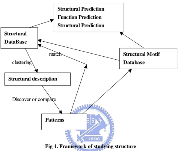
(12) alphabet letters and the local rules for assembly process [15].. Structural Prediction Function Prediction Structural Prediction Structural DataBase match. Structural Motif. clustering. Database. Structural description. Discover or compare. Patterns. Fig 1. Framework of studying structure The framework of studying protein structural was shown as Fig1. The structural description is determined through data mining algorithms and the original sequences will be transformed to those of structural description. The regular pattern or signature will discovered through alignment tools and we could study the relationship of the regular structural pattern and the original sequences. Then, The model of sequence and structures is build by algorithms of prediction. With building model of prediction, we can predict the protein structures from sequences.. 5.

(13) CHAPTER 3: METHODS AND MATERIALS A.. Overview 1. Source files( protein). 2.Local Data Bases 6. Solving Problems with mining tool 3. Data Preprocessing and warehousing. 5. Feature Selection. knowledge. 4. Feature extraction. Fig.2 the overview of our proteomic knowledge base research The Fig.2 show the whole data mining process of constructing the knowledge base. In this thesis, the protein information was gathered from Protein Data Bank (PDB) and saved them into local databases. With data preprocessing methods, I preceded the protein structural information and translated them into our features, like phi, psi, and omega. Besides, the properties of amino acids were collected in our database and joint with our protein database. After preparing these data, we designed the data mining tool to mining the databases with feature selection strategy to construct the protein knowledge. After preparing protein structural database, we began to design the data-mining tool and setup our own knowledge base of proteomic research. The Fig.3 shows the overview of our methods for constructing the knowledge base. Some proteomic researches use the same framework to find the description of protein to setup their own knowledge base. In my thesis, I demonstrated the one data mining tools and its purpose was help researchers to discover the well-represented description of protein structure, sequence, and functionality which can simplify the protein structural and represent the protein structure as different blocks instead of using the three elements, (helices, loop, and sheet) to describe the protein structure. We can compare the description and find 6.

(14) the conserved pattern of transformed-sequences from different proteins structure. More detailed methodology will be shown in the section B to C.. Feature selection. Mining. extract. Algorithms Description of. Structural. features. DataBase mining. comparison. Basic building. Prediction. blocks. Docking Comparison. save Basic building Blocks Database. Fig.3 The detailed framework of our data mining flow After showing the flow of our constructing our knowledge base, we begin to discuss detailed methodology in the following sections. B.. Data Preprocessing. Firstly, we got the raw data from the Protein Data Bank, which is the well-known database. We downloaded them on our local site and parsed them into our own database. The files of Protein Data Bank have its own format (see PDB guide 2.1). According to the guide of protein data bank format, I build the EER model for this Protein Data Bank. I roughly select some title from the protein data bank. I used the PERL program to process these data and saved them into the MYSQL database server. Additionally, the Fig. 3. shows the EER model of our proteomic database. After constructing such the database, we also use some data 7.

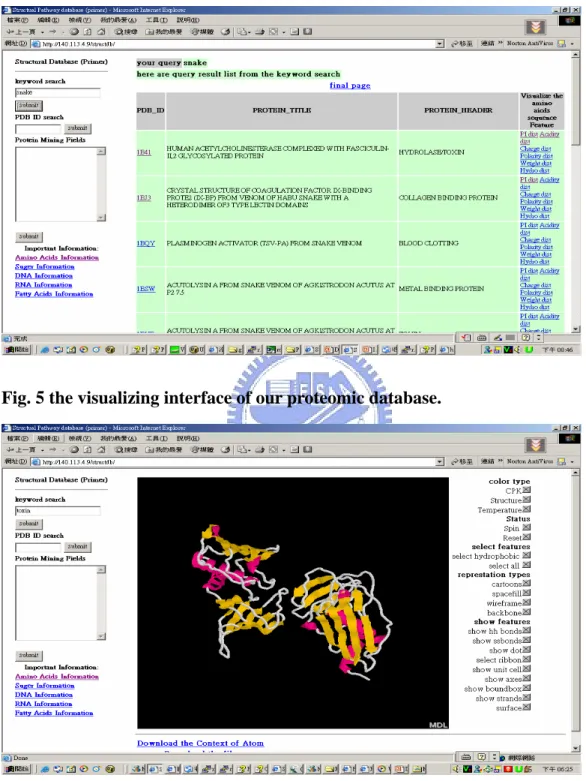
(15) mining technique to extend these EER model. Fig.4 the EER model of our local proteomic database.. In our local database, we also provided some basic query(see Fig. 4.), the web site has provided the keyword query, sequential PDB ID query and PDB ID query for searching the interesting protein. The interface of our database also provided some visualization service (see Fig. 5.) are provide by CHIME plug-in tools. The interfaces also provided some scripts icon to help user realize the property of protein structure. Additionally, it also provided downloading service that you can download the .atom file or the .pdb file from our web site. Moreover, we integrated the Database, Knowledge Base, and mining tools for my research purpose. The integrating the Knowledge Base, mining tools and Database will demonstrate in the Chapter 5. After preparing the database, we calculated the dihedral angle from the atomic coordinates of protein structure and also collected the spatial information and property of 20 Amino Acids. We started designing other tools and setting up our own databases and knowledge base with these protein information. 8.

(16) Fig. 4 the interface of our proteomic database.. Fig. 5 the visualizing interface of our proteomic database.. With this web-based platform, we can study and practice the large protein database management. Also, we can also provide the protein structure researchers a web based platform. C. Proposed combinatorial approach : SUM-K 9.

(17) a. Framework of SUM-K We begin to designing the powerful mining tool to discovering the knowledge from our database and constructing our own Knowledge Base to help researchers realizing the database. The workflow of SUM-K system are shown on Fig. 1. a.Backbone Transformation into Dihedral Angles b.Protein Fragment Vectors Extraction as Input to SOM, i.e. [ψ i − 2 ,φi −1 ,ψ i −1 ,φi ,ψ i ,φi +1 ,ψ i +1 ,φi + 2 ]. c.Train SOM on Protein Fragment Vectors. d.Visualizing trained SOM with U-Matrix in Grey Levels. e.Build Minimum Spanning Tree from U-matrix. f.Partition Minimum Spanning Tree into Disconnected Subtrees. g.Use number of subtrees as K and Run K-mean Algorithm on Input V h.Define Structural Alphabet based on K-means Clusters. i.Transform Proteins into Structural Alphabet Fig. 6. We designed the SUM-K (SOM, U-matrix, MST, and K-means algorithm) 10.

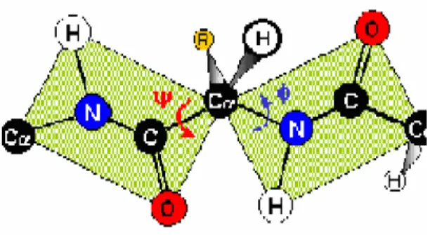
(18) approach based on the Self Organizing Maps and its own visualization methods to discovering the whole new description of protein structure. We can do some value-added visualization on existing database, like SCOP database, and finding the building blocks through the non-redundant proteins with SUM-K. a. Backbone Transformation into Dihedral Angles. Fig. 7 the backbone transformation into Dihedral Angles. The calculation of dihedral angles is shown as follows: (shown as Fig. 7) 1). 2). The Φ angle is the angle between the plane determined by N, Cα, and C of the i th Amino Acids and the one determined by N of i+1 th Amino Acids, Cα, and N of i th Amino Acids. The Ψ angle is the angle between the plane determined by C, Cα, and N of the i th Amino Acids and the one determined by C of i+1 th Amino Acids, Cα, and N of i th Amino Acids.. There are 2 dihedral angles between 2 amino acids. The SOM algorithm clusters the amino acids of the protein according to these three features. In this Thesis, we used the phi and psi angle as our training feature for setting up protein structural alphabet systems and determined the building blocks with SUMK algorithm. b. Protein Fragment Vectors Extraction as Input to SOM. With the fixed window size of five residues, we slid the window along each all-α protein in SCOP, advancing one position in the sequence for each fragment, and collected a set of overlapped 5-residue fragments. As the relation between two successive carbons, Cα i and Cα i +1 , located at the ith and (i+1)th positions, can be. 11.

(19) defined by the dihedral angles ψi of Cα i and φi+1 of Cα i +1 , a fragment of L residues can then be defined as a vector of 2(L-1) elements. Thus, in our study, each protein fragment, associated with α-carbons Cα i − 2 , Cα i −1 , Cα i , Cα i +1 and Cα i + 2 , is represented by a vector of eight dihedral angles, i.e. [ψ i − 2 ,φi −1 ,ψ i −1 ,φi ,ψ i ,φi +1 ,ψ i +1 ,φi + 2 ]. for sliding window size =5. (Shown as following figure.) Based on this representation, we totally gathered 1,143,072 fragment vectors from the all-alpha family in SCOP database. The features are shown as Fig 9.. Fig 8. Showing the dihedral angles we got from the protein structural fragment (window size = 5) c.Train SOM on Protein Fragment Vectors Our tool was based on the Kohonen’s self-organizing maps and use the som-tool-pak 3.1 for our research purpose. The kohonen’s self-organizing map was the unsupervised clustering and it can setup 2D map for representing the relationship of each clusters. The SOM algorithms are shown as follow: 1. Normalize the input data and setup the 2D map with N * M size. 2. Randomly initializing the values of each node on the map. 3. Enter the first training step, (learning steps). The learning rate in this step is higher than that in the second learning step and the purpose of this step is let each unit of the map memorizing the feature of input vector. Through these steps, each output node will be updated by the neighborhood function.. 12.

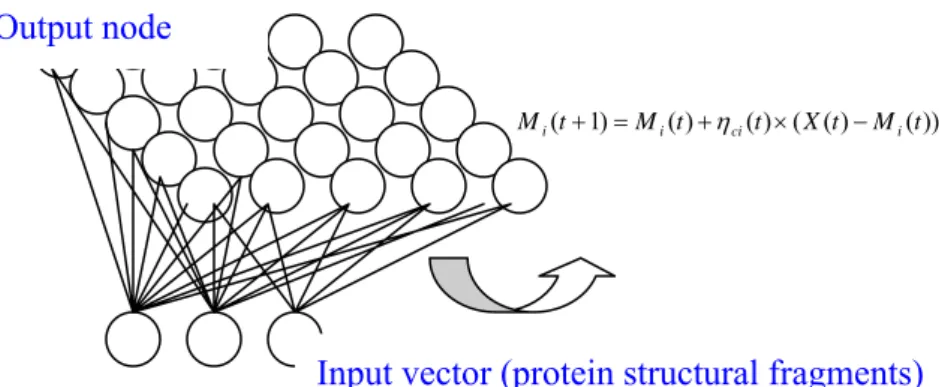
(20) The detailed calculation is shown below: N −1. Di = ∑ ( X (t ) − M i (t )) 2 --------------------------------(1) i =0. We will calculate the Euclidean distance between each input vector and the output map unit and get the nearest map unit C as winner unit. Arg ( Min ( D i )) = C -------------------------------------(2). The input vector the best match node with learning rate will update the winner unit and the neighborhood of winner node will be update by the neighborhood function (shown as formula (3)). After 1000 times later, SOM will converge. The neighborhood function decline through the times and the region of update will be declined also and framework of SOM is shown as Fig 10. M i (t + 1) = M i (t ) + η ci (t ) × ( X (t ) − M i (t )) -----------(3) Where η ci = α (t ) × exp(− Ri − Rc. 2. / 2σ 2 (t )) ------(4). The purpose of first training step maximizes the distance among the centers of cluster 4. The purpose of the next training state is tuning and minimizes the distance of input vectors and the center of cluster. 5. End of the algorithms through the first and second training state. Fig 10. the overview of the SOM clustering algorithms.. Output node M i (t + 1) = M i (t ) + η ci (t ) × ( X (t ) − M i (t )). Input vector (protein structural fragments). 13.

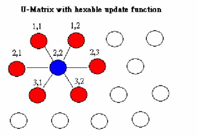
(21) There are 7 parameters was considered to affect the SOM recognize results., They are map size, first learning rate, second learning rate, first training steps, second training steps, update topology, and update function. According to the SOM algorithms, It shows that SOM usually consists of a regular 2D grid of so-called map units, each of which is described by a reference vector mi = [mi1, mi2, mi3,…, mid], where d is the input vector dimension, e.g., d = 8, in our case of fragment vectors. The map units are usually arranged in a rectangular or hexagonal configuration. The number of units affects the generalization capabilities of the SOM, and thus is often specified by the researcher/user. It can vary from a few dozen to several thousands. An SOM is a mapping from the ensemble of input data vectors (Xi=[xi1, xi2, xi3,…, xid] ∈ Rd) to a 2D array of map units. During training, data points near each other in input space are mapped onto nearby map units to preserve the topology of the input space [19][20]. The SOM is trained iteratively. d. Visualizing trained SOM with U-Matrix in Grey Levels. Fig 11. The calculation of U-matrix (take 4X4 SOM map for example). The Unified Matrix (U-matrix) usually used in SOM visualizing researches, and it can reflect the clustering result of SOM. U-matrix is one type of distance matrix that can show the difference between two map units on the SOM maps. Fig 11. is shown the example of calculation the U-matrix on the 4 X 4 SOM maps with hex able topology type. Take the point A (2,2) for example, there are six neighbor map units near the point A was (1,1), (1,2), (2,1), (2,3), (3,1),and (3,2). Each node on the SOM map has six neighbor nodes except the marginal map units and we connected the target point with its neighbor points to constructing connected components for Minimal Spanning Tree. Finally, we constructed the U-matrix which each map units connected with their neighbor map units (shown as Fig 11.) and each connection has 14.

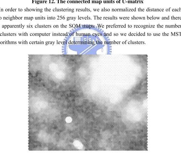
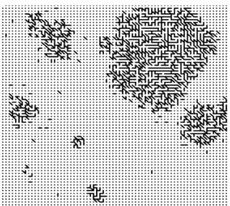
(22) its distances between two nodes. Then, the connected components was produced from U-matrix. (See Fig 12.). Figure 12. The connected map units of U-matrix In order to showing the clustering results, we also normalized the distance of each. two neighbor map units into 256 gray levels. The results were shown below and there are apparently six clusters on the SOM maps. We preferred to recognize the number of clusters with computer instead of human eyes and so we decided to use the MST algorithms with certain gray level determining the number of clusters.. Figure 13. the U-matrix visualization with the 0-255 gray level. f. Partition Minimum Spanning Tree into Disconnected Sub trees. After the above steps, the connected units of SOM maps generated. We used 15.

(23) them as input of Kruskal’s MST algorithm. The MST algorithms will generate the shortest path of connected units of SOM maps. The results were shown as the following Figure.. Figure 14. Formation of Minimal Spanning Tree.. The Fig 14. is shown the completely MST tree of SOM map units. However, the number of clusters should be generated. We defined the threshold value of gray level, which is 47 and cutting the MST tree into several sub trees. After cutting the MST trees, the result of the following can be generated (see Fig 15.). Still, there are still some small sub trees, which are not big enough to form a cluster on the SOM map.. Figure 15. Partition the MST tree into sub trees with gray level 47 16.

(24) To deleting these clusters, the sub trees which size are smaller than (map size) ^1/4 would be excluded and the final MST pruning results was generated (see Fig 16). The following figure was filtered MST pruning results.. Fig 16. Cleaning the MST tree with Tree size < (map size) ^1/4. With the FIND SET Algorithm, the parent of each sub trees and the number of sub trees can be recognized. Then, The number of sub trees means the number of clusters on the SOM map and the number of cluster is generated from this step. With the ability of visualization on the SOM with U-matrix and MST (SUM), the number of clusters preparing for K-means was produced. (See Fig 17). 1 2 4 6. 3 5. Fig 17. Determine the number of clusters on SOM map. 17.

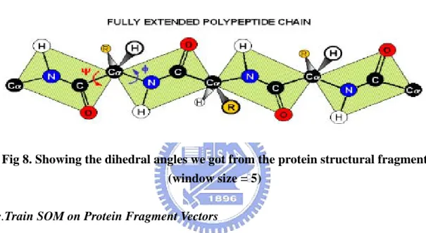
(25) g. Use number of sub trees as K and Run K-mean Algorithm on Input Vectors. Then, the map size expanded from 10X10 to 260 X 260 with SUM till the most frequent number of clusters appeared. The frequent number of cluster is K. We finally take this K as the K parameter of the K-means algorithm. After recognizing the frequent number of cluster, we run the K-means Algorithms with K on input vectors. Because the different random seeds number on the k-means lead different center of clusters, we started to maximize the center of clusters and minimize distance of the input vector and the center of clusters and found the best cluster center as our final clusters center. h. Define Structural Alphabet based on K-means Clusters. We will assign an alphabet to each k-means centers with finding the best cluster center. Then, we reassigned the input vector to the closest centers and give them a alphabet. The formula is shown at h1. Arg ( Min ( D i )) = C -------------------------------------------------------------------------h1. Where Di = Euclidean distance between each center of cluster and input vectors. Through these steps, we can transform raw amino acids sequence to structural alphabet. i. Transform Proteins into Structural Alphabet 10. 20. 30. 40. 50. ---------|---------|---------|---------|---------| SIVTKSIVNADAEARYLSPGELDRIKSFVSSGEKRLRIAQILTDNRERIV aaaaaaaaaaaqqqppphhaaaaaaaaaaaaaaaaaaaaaaaaaaaaaaa 60. 70. 80. 90. 100. ---------|---------|---------|---------|---------| KQAGDQLFQKRPDVVSPGGNAYGQEMTATCLRDLDYYLRLITYGIVAGDV aaaaaaaaqqaaaqqkqhkqwkhhaaaaaaaaaaaaaaaaaaaaaaqqkh 110. 120. 130. 140. 150. ---------|---------|---------|---------|---------| TPIEEIGIVGVREMYKSLGTPIDAVAAGVSAMKNVASSILSAEDAAEAGA aaaaaaqqkhaaaaaaaqqkhhaaaaaaaaaaaaaaaqqkhhaaaaaaaa 160. 18.

(26) ---------| YFDYVAGALA aaaaaaaaaq. Fig 18.transformation the protein raw sequence into our own structural alphabets. After reassigning each amino acids to the center of k-means clusters, the transformed sequences for each protein domain from all-alpha family of SCOP databases was produced. With these sequences we could do the comparative study of different alphabet system with protein structures alignment through 1D structural alphabet sequences.. 19.

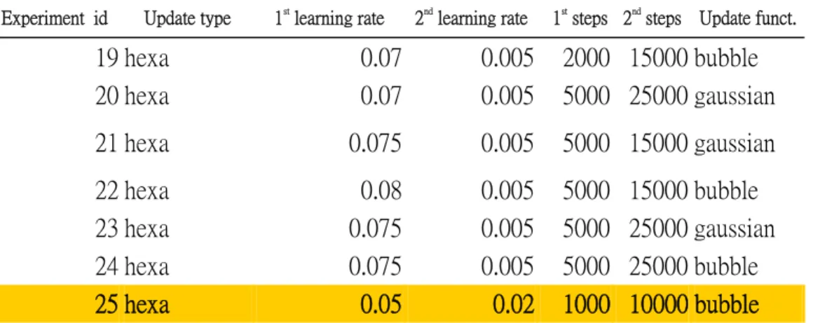
(27) CHAPTER 4: RESULTS AND DISCUSSION. We started to verify the validity of our structural alphabets and tested the parameters of SOM algorithms. Besides, we made discussion of the structural alphabets results and demonstrated the results of structural alphabets. A. Experiments Results and Analysis. In order to finding the optimal combination of each parameters on Self Organizing Maps, we designed the experiment condition for testing the parameters of SOM’s parameters. a. Test the parameters of SOM algorithm We designed 25 combinations of 6 parameters (Table A.) and tested the SOM from map size 10X10 to 100X100. The complete experiment results are shown at Appendix A. We used the about 230 proteins as training data sets and tested our experiments.. Experiment id. Update type. 1st learning rate. 2nd learning rate. 1 hexa. 0.09. 0.01. 2 hexa 3 hexa 4 hexa 5 hexa 6 hexa 7 hexa 8 hexa 9 hexa 10 hexa 11 hexa 12 hexa 13 hexa 14 hexa 15 hexa 16 hexa 17 hexa 18 hexa. 0.09 0.09 0.09 0.08 0.08 0.08 0.08 0.06 0.06 0.06 0.06 0.05 0.05 0.05 0.05 0.07 0.07. 0.01 0.01 0.01 0.01 0.01 0.01 0.01 0.005 0.005 0.005 0.005 0.005 0.005 0.005 0.005 0.005 0.005 20. 1st steps 2nd steps Update funct.. 5000 15000 bubble 5000 5000 5000 5000 5000 2000 2000 2000 2000 2000 2000 2000 2000 3000 3000 5000 5000. 15000 gaussian 25000 bubble 25000 gaussian 15000 bubble 15000 gaussian 25000 gaussian 25000 bubble 15000 gaussian 15000 bubble 25000 bubble 25000 gaussian 15000 gaussian 15000 bubble 45000 bubble 45000 gaussian 15000 gaussian 15000 bubble.

(28) Experiment id. Update type. 1st learning rate. 2nd learning rate. 1st steps 2nd steps Update funct.. 19 hexa 20 hexa. 0.07 0.07. 0.005 0.005. 2000 15000 bubble 5000 25000 gaussian. 21 hexa. 0.075. 0.005. 5000 15000 gaussian. 22 hexa 23 hexa 24 hexa 25 hexa. 0.08 0.075 0.075 0.05. 0.005 0.005 0.005 0.02. 5000 5000 5000 1000. 15000 bubble 25000 gaussian 25000 bubble 10000 bubble. Table A. Test the parameters of SOM algorithms and the 1st radius of update =10 and the 2nd radius of update = 3 a.1.. Condition 1 and 2: comparing the different update function.. Condition 1, map size = 10 X 10. Condition 2, map size = 10 X 10. Condition 1, map size = 50 X 50. Condition 2, map size = 50 X 50. Condition 1, map size = 100 X 100 Condition 2, map size = 100 X 100 Fig 19. The U-matrix result of condition 1 and 2 The gaussian update function can’t get exactly boundary that we can’t use the 21.

(29) MST algorithm to recognize the number of clusters. Instead of gaussain update function, the bubble update function can get the very clearly boundary between two clusters.(see Fig ). a.2.. Condition 1 and 3 ; condition 2 and 4 : comparing the 2nd learning steps. Condition 1, map size = 50 X 50. Condition 3, map size = 50 X 50. Condition 1, map size = 100 X 100. Condition 3, map size = 100 X 100. Condition 2, map size = 50 X 50. Condition 4, map size = 50 X 50. 22.

(30) Condition 2, map size = 100 X 100. Condition 4, map size = 100 X 100. Fig 20. The U-matrix result of condition 2 & 4; 1 & 3 The more 2 learning steps cause the bigger size of cluster, and the results are nd. shown as Fig 20. The clusters in Condition 4 are more aggregated than those in Condition 2. It can be concluded that the 2nd learning steps strongly minimize the distance between the input vector and each cluster centers. (See Fig 20.) a.3.. Condition 18 and 19: comparing the 2nd learning steps. Condition 18, map size = 10 X 10. Condition 19, map size = 10 X 10. Condition 18, map size = 50 X 50. Condition 19, map size = 50 X 50. 23.

(31) Condition 18, map size = 100 X 100. Condition 19, map size = 100 X 100. Fig 21. The U-matrix results of condition 18 & 19 Fig 21. is shown that the more 1st learning steps lead the map unit learning more clustering centers. These centers are very closely to other neighbor nodes. In the other. words, running more first learning steps makes more map units learn specific center of cluster and the boundary of each cluster centers become clearer. a.4. Condition 10 and 19: comparing the 1st learning steps. Condition 10, map size = 10 X 10. Condition 19, map size = 10 X 10. Condition 10, map size = 50 X 50. Condition 19, map size = 50 X 50. 24.

(32) Condition 10, map size = 100 X 100. Condition 19, map size = 100 X 100. Fig 22. The U-matrix results of condition 10 and 19 The lower 1st learning rate cause the more exactly boundary. We observed that. Learning rate in Condition 10 is lower than Learning and boundary of maps in Condition 10 is more clearly than Condition 19. (See Fig 22.) Based on the above phenomenon, it means that 1st learning rate affect the number of clusters you will determine. Therefore, The more 1st learning rate cause each node could learn strongly in each step of SOM training. Then, the map becomes unstable and fuzzier in higher1st learning rate.. 25.

(33) a.5.. Condition 22 and 5: comparing the 2nd learning rate. Condition 22, map size = 10 X 10. Condition 5, map size = 10 X 10. Condition 22, map size = 50 X 50. Condition 5, map size = 50 X 50. Condition 22, map size = 100 X 100. Condition 5, map size = 100 X 100. Fig 23. The U-matrix results of condition 22 & 5. The boundary of cluster in Condition 22 is clearer than Condition 5. (See Fig 23.). We supposed that the lower 2nd learning rate cause each map units learning slowly and the distance between the input vector and the cluster center can’t be minimized effectively. In order to improving the boundary of cluster to become more clearly, the more 2nd learning steps or higher learning rate is proposed.. 26.

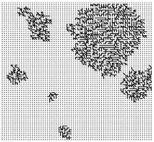
(34) a. 6 Condition 15: comparing the effect while map size changed.. Map size: 10 X 10. Map size: 30 X 30. Map size: 60 X 60. Map size: 100 X 100 Fig 24. The U-matrix result of different map size in condition 25 Fig 24. is shown the different map sizes: 10X10, 30X30, 60X60, and 100X100. While increasing the map size, the boundary of clusters is clearer. It is just because. the cluster could find a position and distinguish from the other clusters. Because the condition 25 is much better than the others, we begun to use the condition 25 to do our experiment and construct our own structural alphabets with SUM-K. 27.

(35) a.7 verify each white region contains only one clusters with k-means.. In order to represent a white region is only one cluster, we use the K means algorithm to do such verification.. 2. 5 4. 1 3. 3. 1. 2. 4 5. Condition 5 map size = 100X100. K – means where k = 5. Fig 25. The U-matrix result of condition 2 & 4 ; 1 & 3. Take Condition 5 as an example, there are five clusters on the map and we use the k-means algorithm to verify them. The five clusters exactly match the white block and it can prove that there are five clusters on training data sets. We can conclude from this experimental section that the clustering number can be generated from the SOM and U-matrix algorithms, each white block could represent a distinguish cluster. With this observation, we can implement the MST algorithms and generate the sub trees with threshold of lower gray level. Then, we selected the threshold of gray level and took this number as the number of clusters to finding the center of clusters. The SUM, which contains SOM, U-matrix, and MST was proposed to analyze the number of clusters. b. Expansion test of SOM maps and get the number of clusters.. We started the SUM-K approach. Firstly, We trained the SOM map with the all-alpha family data, and did the experiment of expanding the map size of SOM from 10 nodes times 10 nodes to 240 nodes times 240 nodes. While the training steps finished, we fixed the threshold on gray level = 47 and pruned the connection of MST. The number of clusters determined by MST was unstable while the map size under the 80 nodes times 80 nodes (see Fig 26 and point 2). Besides, There is an extremely different point is 30 X 30 (see Fig 26 and point 1). It shows that there are about 16 28.

(36) clusters on the map. Then, the next point (60 X 60) declined to 6 clusters. The different of number of clusters was 10. The chart was revealed that under the 80X80 size of SOM map and the number of clusters performed unstable and we can’t recognize the number of clusters through these points. However, while the map size is bigger than 80 X 80, it shows the number of cluster become more stable and they fixed between 10 and 12. Then, the number of clusters can be generated from SOM and it was 11. With observing the result of the expanding the SOM map we determined the number of clusters from the SOM. 1. number of cluster. 20. 10. 21 0X 21 0. 60 16 0X 1. 11 0X 1. 60 X6 0. 0 10 X1. 10. 2. 0. map size. Fig 26. map size versus number of clusters. Besides, in order to determining the number of clusters, we drew the graph of frequency versus the number of clusters.(see Fig 27.). The peak is 11, too. We use the k = 11 for k-means algorithms Peak (cluster =11) 7. frenquency. 6 5 4 3 2 1 0 1. 6. 11. 16. 21. number of cluster. Fig 27. number of cluster versus frequency 29.

(37) 16. 0. 16. 0X 11. 0X. 11. 0 X6 60. X1 10. 0. 35000 30000 25000 20000 15000 10000 5000 0 0. number of cluster. c. using the negative data set for test.. map size. Fig 28. map size versus number of clusters (negative data sets). In order to proving our number of clusters couldn’t be recognized exactly by data sets produced randomly, we produced the negative data sets that generated from the original data sets. We added the original input vectors randomly between 30 and -30 and generated the negative data set. Though it’s not reasonable to produce these data, the purpose of this experiment is to proving that the negative data set couldn’t generate the certain number of cluster by our SUM-K approach. The result of experiment has shown that while map size is smaller than 60X60 the number of cluster is 1. It means the SOM couldn’t recognize the clusters and gather all data sets into one clusters. However, while map size is bigger than 60X60, the number of clusters will increase highly and become unstable than the original data sets produced. It just because that the map size is big enough to cover all the data sets, the SOM map units can catch one input vectors and these vectors may be recognize as one cluster. Therefore, our SUM-K is valid and reasonable through this experiment. d. With-in cluster and between clusters analysis. After we verified our number of clusters is valid and reasonable, we ran k means algorithm and found the best center by minimize the distance of within clusters and maximize the distance of between clusters. We repeated the k-means cluster 250 times and find the best result of clusters center. (See Table B.) 30.

(38) The table is the best result of centers and we use these centers as our cluster center. Then, we showed the mean and standard deviation of within clusters and between clusters. We assigned the number of clusters to alphabets from A to K and transformed from the original sequences to the sequences of structural alphabet. Table B. within clusters and without clusters analysis.. within-cluster. J. I. H. G. F. E. D. C. B. A. 43.15±50.13. 88.77±53.33. 196.75±97.2. 155.02±77.8. 220.52±87.79. 143.62±90.84. 150.41±71.53. 193.67±69.19. 173.58±77.59. 192.84±74.97. 186.10±68.07. mean±sd. K. A. 0. B. C. D. E. G. center-to-center F. H. I. J. K. 226.52. 86.711. 358.58 360.95. 335.84 136.63 164.87. 343.07 276.03 341.22 278.5. 346.14 220.63 346.98 161.11 177.48. 302.93 511.04 284.51 343.02 282.19 358.48. 234.31 252.05 388.9 261.9 323.81 183.77 233.33. 250.31 251.6 197.76 383.86 243.02 333.41 188. 284.59 203.41 202.8 275.08 414.99 169.3 321.03 208.28 264.69. 282.3 205.27 216.75 226.93 236.72 399.53 246.5 325.94 197.44 245.81 0. 0. 0. 0. 0. 0. 0. 0. 0. 0. 31.

(39) B. Comparing the different SAs and homologous finding tool –FASTA and BLAST. Transformation of raw sequence to SUMK structural alphabet system. Print the sequence data in the txt file.. Randomly select the query protein from the protein structures (sequence identity < 30%). run homologous search with BLAST and BLOSUM 62 (for Amino Acids sequences) FASTA and IDENTITY (for. Repeat 1000 times. de Brevern, SUMK, and 2 level SOM). Choose the highest one of subject protein and do RMSD, hierarchical matching with query protein. Fig 29. The overall flow of comparative study of different alphabets system. We clustered the raw data with K- means which k parameter of k-means is 11 and gave the 11 alphabets to representing each cluster of k-means. Proteins of the all-alpha family from SCOP database were clustered according to the features. We assigned the protein sequences in our own structural alphabet and saved them in our own database. We used the FASTA algorithm with Identity matrix in our own structural alphabet systems to prove that our structural alphabet is meaningful and can distinguish the protein family from SCOP database. Besides, FASTA algorithms and Identity matrix can determine the similarity of two sequences and it also gave the most similar subject sequence to the query sequence from our own database. Running the comparative experiment, Mode Carlo method was used to verifying our own alphabet is practical. We randomly selected one protein as the query protein and randomly select 1000 other proteins as the subject proteins from all-alpha family in SCOP database. In this step, we used the FASTA and Identity matrix we proposed before to calculate the similarity between query and subject sequences. Then, we selected the top one and calculated the hits of SCOP database 32.

(40) hieratical relationship. There are four types of hits in our experiment. The first type is hit the most top level-class, the second type is hit the second level -- fold, the third type is hit the third level –super family, and the fourth type is hit the bottom level – family of SCOP database. For example, the top one of subject proteins is a.1.1.1 and the query one is a.1.1.2, the type of hit is super family. The best type of hit is the fourth type. It’s just because this type completely match the hieratical relationship of SCOP database. This experiment repeated 500 times, and each time we selected the top one and determined the type of hits that our own alphabet catches. The overall flow of experiment was shown as Fig 25. As for the other structural alphabet system, we tested alphabets of the Amino Acids, de Brevern, and the 2-level SOM with the same procedure. Thus, the Amino Acids do the homologous search with the BLAST and BLOSUM 62 matrix while the other three alphabets do the similarity search with the FASTA and Identity matrix. a. SCOP hierarchical matching frequency at different level. Method. class. fold. BLAST. 71. 4. 5. 20. SMK. 55. 11. 5. 29. de Brevern. 58. 4. 11. 27. 2-level SOM. 73. 6. 14. 7. super family. family. Table C. hierarchical matching results.. The de Brevern work has defined the structural alphabet system, we transformed the proteins of all-alpha family from SCOP database into their own alphabet and run the experiment of verification described in the section B. we started to compare the different of these two alphabet systems. There are 16 structural alphabets under HPM methods and we saved the transformed sequences in our databases. Also, we saved sequences of 2-level SOM and Amino Acids The results revealed (See Table C.) that our SUM-K’s alphabets with FASTA and IDENTITY matrix can catch more SCOP family hierarchical than the others while the identity of sequence lower than 30 percents. Then, the performance of 2-level SOM approach couldn’t catch the SCOP hierarchical well. The BLAST and BLOSUM 62 matrix can catch the SCOP hierarchical better 33.

(41) than 2-level SOM alphabets. The de Brevern universal structural alphabet with FASTA and IDENTITY search perform better than BLAST homologous search with Amino Acids sequences. However, the overview of SCOP hierarchical can’t match well, there are still many mismatch in our experiments. It may be the SCOP databases may contain the other information like functional and sequential information besides the structural information. Therefore, we used the RMSD measurement to recognize the ability of structural presentation of our structural alphabet and other three alphabets. b. RMSD analysis of different Structural Alphabets. method. Mean (RMSD). sd (RMSD). BLAST. 8.953744. 4.764597. SMK. 7.290972. 3.934283. de Brevern. 8.076746. 4.819178. 10.38624 5.217078 2-level SOM Table D. hierarchical matching results. We used the RMSD measurement to comparing the similarity of the best subject and the query protein structures. According to this tables, our structural alphabet can represent the protein structure well than the other structural alphabets and the deviation of RMSD was smaller than the other three alphabets. In this experiment, we can conclude that our structural alphabet is better than the other three alphabets and we have found the protein building blocks of all-alpha family through this experiment. C.. Visualization of SUM-K results. After serial verification experiments, we can declare we have found better structural alphabet than the other structural alphabet system. We also used the Rasmol to showing the structural building blocks and the Swiss PDB to do super position with 30 protein fragments in the same clusters. These results represented the characteristics of protein fragments and were shown as Table E and F. 34.

(42) A. B. C. D. E. F. G. H. I. J. K Table E. Visualize the wire frame of each clusters (super position) 35.

(43) A. B. C. D. E. F. G. H. I. J. K Table F. Visualizing the backbone of each clusters. 36.

(44) CHAPTER 5: APPLICATION A. Valued-Add on the Protein Data Base and Service on the Web. We provide the service of protein database and our mining tool on the web. (see Fig 30.). Fig 30. Main page of our SUM-K web service You can query the protein database from our own site and we also provide some. visualization tools. The following tables are the service we provide and demonstrate the interface for mining the protein databases.. Fig 31.Main page of protein DB and KB. Fig 32.Query protein from local database. Fig 33.visualization. Fig 34.Data mining mode. 37.

(45) Fig 35. Configuration of the SUMK parameters. Fig 36. The clustering result and get the information of structural alphabet. Fig 37.Use the rasmol from result of SUMK. Fig 38.Demonstrate the SOM clustering result of SUMK. Fig 39. Demonstrate the SOM k means verification result. You could enter the normal query page (see Fig 31) for searching the basic protein description and get the structure information from the web based platform. After querying a protein, you could click the hyperlink of PDB ID to see the visualization of protein structure. (Fig 32, Fig 33). Additionally, our web site provides the mining process (SUM-K approach) for user to study the protein structural information. (Fig 34.) You could input your proteins in specific format to query the protein you want to do data mining analysis. 38.

(46) After you choose the proteins you want to training, you’ll enter the page that contains configuration of SUMK approach for protein. (Fig 35.). After you input the parameters, the server will start to run analysis of the protein data. Then, you will get the unique serial number that you can enter protein structural analysis platform and do four kinds of analyses. They are: 1. Show all results of SUM-K 2. Show the SOM and k-means results of SUM-K 3. Show the SOM and MST clustering result of SUM-K 4. Labeling the structure with SUM-K result You can get the complete information of SUM-K from the first service (Fig 36). Both the information of protein sequences and the labeling information of Rasmol scripts you’ll get from the web site. While you got this information, you can enter the fourth service and label the structure according to our structural alphabet. (Fig 37). In order to see the verification of your clustering results, you can use the second service to read information of k-means clustering results and cluster verification of SOM maps. (Fig 38) Besides, you can see the result of number of clusters and decide the number of gray level threshold through the third service. It can help you to decide the flexibility of cutting the MST trees and get better result. (Fig 39). 39.

(47) CHAPTER 6: FUTURE WORKS. With SUM-K, we have set up our structural alphabet representation system from the all-alpha family in SCOP database. We also proved that our alphabet system is meaningful through the serial experiments. The SUM-K approach can catch the proper size of structural alphabets. We will run SUM-K approach with non-redundant protein chains and find the universal structural alphabets. Besides, we will learn the profile of structural alphabets and amino acid sequences with Bayesian or HMM model and build the model for structural prediction. We will maintain the protein data base and do the structural research with our universal structural alphabet.. 40.

(48) CHAPTER 7: ACKNOWLEDGEMENTS. I was deeply appreciative of professor Hu and professor Yang provided the opportunity to let me realize the methodology of research. I specially thank that professor Hu provided the precious suggestion on our research; Yang supported the enough resources used and Hwang’s valuable suggestion in my proteomic research.. 41.

(49) CHAPTER 8: PREFERENCE. [1] D. Baker and A. Sali, “Protein Structure Prediction and Structural Genomics”, Science, vol. 294, 2001, pp. 93-96. [2] A.G. de Brevern and S.A. Hazout, “Hybrid Protein Model(HPM): a method to compact protein 3D- structure information and physicochemical properties”, IEEE Comp. Soc. S1, 2000, pp. 49-54. [3] C.A. Orengo, J.E. Bray, T. Hubbard, L. LoConte and I. Sillitoe “Analysis and assessment of ab initio three-dimensional prediction, secondary structure, and contacts prediction”, Protein, vol. 37, 1999, pp. 149-170. [4] J. Garnier, D. Osguthorpe and B. Bobson, “Analysis of the accuracy and implications of simple methods for predicting the secondary structure of globular protein”, Journal of Molecular Biology, vol. 120, 1978, pp. 97-120. [5] B. Rost and C. Snader, “Prediction of protein secondary structure at better than 70% accuracy”, Journal of Molecular Biology, vol. 232, 1993, pp. 584-599. [6] A. Salamov and V. Solovyev, “Protein secondary structure prediction using local alignments”, Journal of Molecular Biology, vol. 268, 1997, pp. 31-36. [7] T.N. Petersen, C. Lundegaard, M. Nielsen, H. Bohr, J. Bohr, S. Brunak, G.P. Gippert and O. Lund, ”Prediction of protein secondary structure at 80% accuracy”, Proteins, vol. 41, 2000, pp. 17-20. [8] B. Rost, “Review: Protein secondary structure prediction continues to rise,” Journal of Structural Biology, vol. 134, 2001, pp. 204-218. [9] A.G. de Brevern, H. Valadie, S.A. Hazout and C. Etchebest, “Extension of a local backbone description using a structural alphabet: A new approach to the sequence-structure relationship,” Protein Science, vol. 11, 2002, pp. 2871-2886. [10] R. Unger, D. Harel, S. Wherland and J.L. Sussman, “A 3D building blocks approach to analyzing and predicting structure of proteins”, Proteins, vol. 5, 1989, pp. 355-373. [11] J. Schuchhardt, G. Schneider, J. Reichelt, D. Schomburg and P. Wrede, “Local structural motifs of protein backbones are classified by self-organizing neural networks”, Protein Engineering, vol. 9, 1996, pp. 833-842. [12] M.J. Rooman, J. Rodriguez and S.J. Wodak, “Automatic definition of recurrent local structure motifs in proteins”, Journal of Molecular Biology, vol. 213, 1990, pp. 327-336. [13] J.S. Fetrow, M.J. Palumbo and G. Berg, “Patterns, structures, and amino acid frequencies in structural building blocks, a protein secondary structure classification scheme”, Proteins, vol. 27, 1997, pp. 249-271. 42.

(50) [14] C. Bystroff and D. Baker, “Prediction of local structure in proteins using a library of sequence-structure motif”, Journal of Molecular Biology, vol. 281, 1998, pp. 565-577. [15] A.C. Camproux, R. Gautier and P. Tuffery, “A hidden Markov model derived structural alphabet for proteins”, Journal of Molecular Biology, doi: 10.1016/j.jmb.2004.04.005. [16] A.G. de Brevern, C. Etchebest and S. Hazout, “Bayesian probabilistic approach for predicting backbone structures in terms of protein blocks”, Proteins, vol. 41, 2000, pp. 271-287. [17] J.A. Hartigam and M.A. Wong, “A k-means clustering algorithm”, Applied Statistics, vol. 28, 1975, pp. 100-108. [18] K.T. Simons, I. Ruczinski, C. Kooperberg, B.A. Fox, C. Bystroff and D. Baker, “Improved recognition of native-like protein structures using a combination of sequence-dependent and sequence-independent features of proteins”, Proteins, vol. 34, 1999, pp. 82-95. [19] J. Vesanto and E. Alhoniemi, “Cluster of the self-organizing map”, IEEE trans. Neural Networks, vol. 11, 2000, pp. 586-600. [20] T. Kohonen, “Self-organizing Maps”, Berlin/Heidelberg, Germany; Springer, Vol. 30, 1995. [21] P. Tamayo, D. Slonim, J. Mesirov, Q. Zhu, S. Kitareewan, E. Dmitrovsky, E.S. Lander and T.R. Golub, “Interpreting patterns of gene expression with self-organizing maps: Methods and applications to hematopoietic differentiation”, PNAS, vol. 96, 1999, pp. 2907-2912. [22] J. Iivarinen, T. Kohonen, J. Kangas and S. Kaski, ”Visualizing the clusters on the self-organizing map”, in Proc. Conf. Artificial Intelligence Research Finland, 1994, pp. 122-126.. 43.

(51) Hexa 0.08 0.01 5000 15000 bubble (start). Hexa 0.09 0.01 5000 15000 bubble (start).

(52) Hexa 0.09 0.01 5000 25000 bubble (start).

(53) Hexa 0.08 0.01 5000 15000 gussain (start).

(54) Hexa 0.09 0.01 5000 15000 gaussain(start).

(55) Hexa 0.09 0.01 5000 25000 gaussain (start).

(56) hex 0.08 0.01 2000 25000 gaussain (start). Hex 0.08 0.01 2000 25000 bubble (start).

(57) Hex 0.06 0.005 2000 15000 gaussain (start).



(60) Hex 0.05 0.005 2000 15000 bubble (Start).

(61) Hex 0.05 0.005 2000 25000 bubble (start). Hex 0.05 0.005 2000 25000 gaussain (start).

(62) Hex 0.06 0.005 2000 15000 bubble (start).

(63) Hex 0.06 0.005 2000 25000 bubble (start).

(64) Hex 0.07 0.005 2000 15000 bubble (start).

(65) Hexa 0.07 0.005 5000 15000 bubble(start).

(66) Hex 0.07 0.005 5000 15000 gaussain (start). Hex 0.07 0.005 5000 25000 gaussain (start).


(68) Hex 0.075 0.005 5000 15000 bubble (start).


(70) Hex 0.075 0.005 5000 25000 bubble (start).

(71)

(72)