基於細胞神經網路的仿生型電腦視覺系統

(1)

1

基於細胞神經網路的仿生型電腦視覺系統

Bionic Computer Visual System

based on

Cellular Neural Networks

研究生：黃朝暉 Student：Chao-Hui Huang

指導教授：林進燈博士 Advisor：Dr. Chin-Teng Lin

國立交通大學

電機與控制工程學系

博士論文

A Dissertation

Submitted to Department of Electrical and Control Engineering

College of Electrical Engineering and Computer Science

National Chiao-Tung University

in partial Fulfillment of the Requirements

for the Degree of

Doctor of Philosophy

in

Electrical and Control Engineering

June 2007

Hsinchu, Taiwan

(2)

2

基於細胞神經網路的仿生型電腦視覺系統

學生：黃朝暉指導教授：林進燈

國立交通大學電機與控制工程學系﹙研究所﹚博士班

摘要

自從 Dr. Ramón y Cajal 開始了對視覺神經細胞的研究以來，包含了眼球與大腦的人類視覺系統（Human Visual System）就成了一個有趣的研究主題。許多學者們也已提出了他們的研究成果並指出了一些新的研究議題。至目前為止，人類視覺系統與其生理結構已經大概被了解了。一些神經學家也已經開始分析人類視覺系統在神經學上的機制。然而，由於人類視覺系統相當龐大且複雜。至目前為止，我們仍然尚無法完全地了解、分析、甚至是模擬它。

視覺資訊 (Visual Information) 的旅程始於視網膜。過去數十年來人們相信視網膜的作用就如同照相機的感光底片。實際上，視網膜的功能遠超過我們已經知道的。根據 Werblin 與 Roska 在 2005 年的研究，視網膜提供了相當巨量的視覺前處理 (Preliminary Visual Processing)。在視網膜中，視覺資訊首先被光感受體 (Photo-receptor) 所接收。接下來經過一連串的視覺細胞的協同作用後，處理過的視覺資訊被分成超過 12 個不同的頻道並同時透過視神經節即時地傳送到視覺大腦皮質層作更進一步的處理。

延續這些學者的研究成果，本論文提出了一個基於細胞神經網路 (Cellular Neural Networks) 的仿生型電腦視覺系統 (Bionic Computer Visual System)。本系統包含了兩個模型，分別是視網膜中央小窩電腦計算模型（Computer Fovea Model），與視覺大腦皮質層電腦計算模型 (Computer Cortex Model)。這兩個模型均是基於人類視覺系統而開發。其中大部份並以

(3)

3 細胞神經網路加以實現。

為了將所提出的模型以細胞神經網路加以實現，本論文亦提出了一些使用細胞神經網路處理影像的新方法。為了達到與生物體結構一致，本論文提出了一個以六角形狀排列的細胞神經網路 (Hexagonal-type Cellular Neural Network)。同時亦提出將在本研究中被應用的數種基於細胞神經網路的穩態中央線性系統 (Stable Central Linear System of Cellular Neural Networks) 的演算法；包括了 CNN-based Laplace-type Filtering 、 CNN-based Gaussian-type Filtering、與 CNN-based Gabor-type Filtering。這些演算法將成為所提出的視網膜中央小窩電腦計算模型與視覺大腦皮質層電腦計算模型的基本元件。

視網膜中央小窩電腦計算模型可用於模擬某些視網膜的生理結構。透過研究以及模擬這些生理結構，一些人類視覺系統的特性可以被模仿出來。這些特性形成了天然的影像強化機制。因此可以使用所提出的架構來重現這些影像強化機制。這些機制包括了色彩統一性處理 (Color Constancy) 與影像銳化處理 (Image Sharpness)。

視覺大腦皮質層電腦計算模型可用於模擬某些處理視覺的腦皮質區。其提供了簡單的影像紋理辦識及聯想的機制。透過研究腦部視覺皮質區的作用，部份人類視覺系統處理影像紋理的機制也可以被模擬出來。這些機制包含了影像紋理隔離 (Segregration) 、分類 (Classification)、以及辦識 (Identification)。透過了解這兩個電腦計算模型，部份人類視覺系統中有意義的功能可以被研究、學習、甚至是被模仿。因此，本研究可以提供人機界面領域 (Human-Computer-Interaction) 的研究一個新的方向。

(4)

4

Bionic Computer Visual System based on Cellular Neural Networks

Student：Chao-Hui Huang Advisors：Dr. Chin-Teng Lin

Department of Electrical and Control Engineering

National Chiao Tung University

ABSTRACT

A Human Visual System, including the eyes and the brain, is always an interesting research topic. Since Dr. Ramón y Cajal initialed the study of the visual neurons, many researchers introduced their research results and indicated more and more issues. Currently, the Human Visual System and its biological structure has been roughtly understood. Some neurologists also started to analyze the neurological mechanisms of the Human Visual System. However, the Human Visual System is an extremely huge and complex system; we are not able to fully analyze, to understand, or even to simulate it, yet.

The journey of visual information is started at a retina. For dacades, people believe that the retina is similar to the silver pieces in the film of a camera that react to light. In fact, the functions of the retina are much more than what we already knew. According to Werblin and Roska (2005), the retina provides a huge number of preliminary visual processings. In the retina, first, the visual information has been accepted by the photo-receptors. After the co-operations of some visual neurons have been finished, the visual information is separated into more than 12 channels and are transmitted to the visual cortex of the brain via some neural axises for further processing in real-time.

(5)

5

Following the works of those researchers, in this thesis, a Bionic Computer Visual System based on Cellular Neural Networks (CNNs) has been introduced. This system includes two major parts: a Computer Fovea Model and a Computer Cortex Model. Those two models are based on the biological structures of the Human Visual System and they are implemented based on the Cellular Neural Networks.

For the sake of implementing the proposed models on the Cellular Neural Networks, some advanced approaches for CNN-based image processing are also introducted. In order to consist with the biological structures, a hexagonal-type Cellular Neural Network is introduced. Meanwhile, some operators, which are based on the Stable Central Linear System of the Cellular Neural Networks, are also presented and are used in this thesis. Those operators include CNN-based Gaussian-type filtering, CNN-based Laplace-type filtering and CNN-based Gabor-type filtering. They became the fumdental elements of the proposed Computer Fovea Model and the Computer Cortex Model.

The Computer Fovea Model can be used to simulate the preliminary processing of a retina. Through investigating this model, various properties of the Human Visual System can be simulated. The Human Visual System possesses numerous interesting properties, which provide the natural methods of enhancing visual information. Various visual information enhancing algorithms can be developed using these properties and this model. The proposed algorithms include color constancy, image sharpness.

The Computer Cortex Model provides simple texture recognition and association for the textures on an image. Through investigating the behaviors of this model, some properties of the texture analysis of the Human Visual System also can be simulated, including texture segregation, classification, and identification.

(6)

6

System can be investigated, understood, even simulated. Thus, this study can provide a new method for the field of Human-Computer-Interaction.

(7)

7

ACKNOWLEDGEMENTS

首先感謝指導教授林進燈多年來的指導。對於本論文的完成，除了林教授的指導以外，也非常感謝諸位口試委員寶貴的意見，使得本論文更加完備。此外，感謝 Professor Leon Chua 在學生赴美期間的指導，以及 Professor Harri Reddy、Professor Tamas Roska、Professor Hyongsuk Kim、Dr. Casaba Rekeczky、Dr. Heinz Koeppl、Dr. Sook Yoon、Dr. Heather Levien 等前輩在學生赴美期間給與許多生活與課業上的協助。在學校方面，感謝蒲博士鶴章學長、劉博士得正學長、鄭博士文昌學長、張博士俊隆學長、世安、政宏等同學在學業上與生活上的幫忙與照顧。最感謝的，是家人的支持。雙親黃連山與黃林淑香多年來無悔的付出。大姐黃慧寧、大姐夫黃一晢、二姐黃慧雯在經濟上的全力支援，以及未來的牽手周惠美長年以來的支持與鼓勵，使得我無後顧之憂的專心於學業。謹以本論文獻給我的家人與關心我的師長與朋友們。

(8)

8

LIST OF FIGURES

Figure 2-1. (a) Architecture of CNN; (b) Dynamic route of states in CNN. 27 Figure 3-1. Distribution of cones on the retina of mammalian. 54 Figure 3-2. The comparison between different layout of CNNs, where (a) is rectangular

8-connected rectangular-type CNN, (b) is rectangular 4-connected rectangular-type CNN, and (c) is hexagonal 6-connected hexagonal-type CNN. 54 Figure 3-3. The confliction of connection in diagonal direction of 8-connected CNN. 55 Figure 3-4. Hexagonal-type image sampling and indexing scheme. 55 Figure 3-5. An example of hexagonal-type CNN implementation based on rectangular-type

CNN. For each cells, the upper-left and lower-right direction of synapses has

been disconnected. 55

Figure 3-6. The sampling method of proposing model. 56

Figure 3-7. The geometrical relationship among pixels, where the error of distance between

different directions is about 11.8%. 56

Figure 3-8. The sampling pixel we used in this section, where (a) is rectangular-type pixel,

and (b) is hexagonal-type pixel. 56

Figure 3-9. The comparison of artificial images between the image which has been constructed by square-shape pixels and the image which has been constructed

by hexagonal-shape pixels. 57

Figure 3-10. The example of different type of sampling methods, where (a) is the rectangular-type image, (b) is hexagonal-type image, (c) and (e) show the details of (a), (d) and (f) show the details of (b). 57 Figure 3-11. The processing result of hCNN-based Gabor-type filtering, where (a) is the

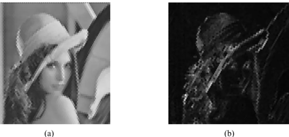
input hexagonal-type image and (b) is the output. Note that the resolutions of the images have been reduced and therefore the hexagonal pixels can be exposed. 58 Figure 3-12. The schematic of Horn’s model using summing and threshold elements. The

feedforward structure calculates the Laplace operator, while the feedback loop structure calculates the inverse Laplace operation. Note that for the shake of clarity of the figure not all the feedback and feedforward interconnections are indicated. This figure has been obtained from [45]. 58 Figure 3-13. The processing result of hCNN-based Retinex-model, where (a) is the input

hexagonal-type image, and (b) is the output. 58

Figure 3-14. The example of different type of sampling methods, where (a) is the original image, (b) is the image which has been sampled by the rectangular-type method, and (c) is the image which has been sampled by the hexagonal-type method. 59 Figure 3-15. The result of comparisons, where (a) is the error between the original image and

(11)

11

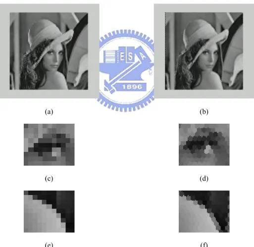
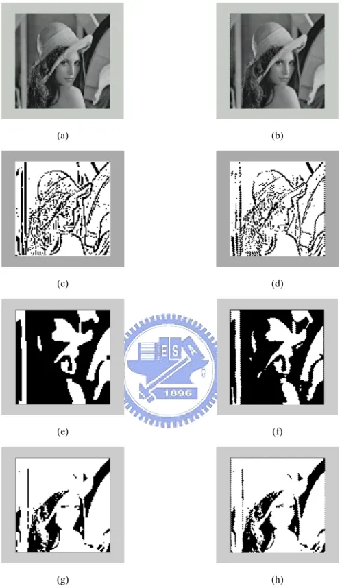
hexagonal-type image. Clearly, the error between the original image and hexagonal-type image is smaller than the other. 59 Figure 3-16. Experimental results were shown in this figure, where (a), (b) are the input

images for the rectangular-type CNN and the hexagonal-type CNN respectively. First, (c) and (d) are the output images processed by the rectangular-type CNN and the hexagonal-type CNN, respectively, where they present CONTOUR_DETECTION function. Next, (e) and (f) are as same as the above and they present SMOOTHING_with_BINARY_OUTPUT function. Finally, (g)

and (h) present BINARY_THRESHOLDING function. 60

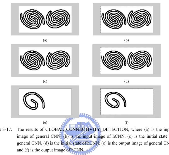
Figure 3-17. The results of GLOBAL_CONNECTIVITY_DETECTION, where (a) is the input image of general CNN, (b) is the input image of hCNN, (c) is the initial state of general CNN, (d) is the initial state of hCNN, (e) is the output image of general CNN, and (f) is the output image of hCNN. 61 Figure 4-1. The biological structure of the photoreceptors in the fovea of a mammalian,

where (a) represents the photoreceptor group in a fovea and (b) represents that the photoreceptors can be classified according to the stimulation they react to [1]. 74 Figure 4-2. An example of a ganglion, where (a) represents that a ganglion collects

information from a set of neighboring photoreceptors. The response of the central part of the set differs from that of the peripheral part of the set. Based on the difference between the types of photoreceptor, ganglion can be classified into red-green (RG), blue-yellow (BY), and black-white (BW) types. Meanwhile, (b) shows the RF of a center-green-on/surround-red-off ganglion, and (c) shows the RF of a center-yellow-on/surround-blue-off ganglion. 74 Figure 4-3. Based on the different responses of neighboring ganglions, the visual

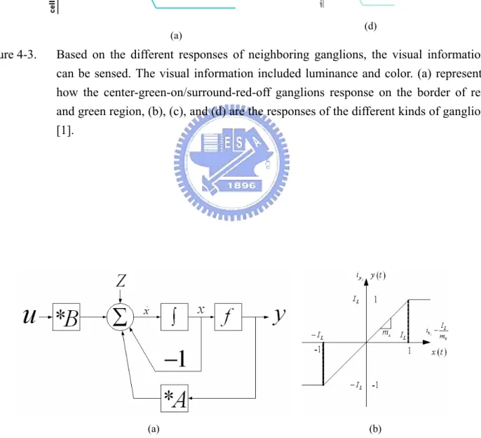
information can be sensed. The visual information included luminance and color. (a) represents how the center-green-on/surround-red-off ganglions response on the border of red and green region, (b), (c), and (d) are the responses of the different kinds of ganglion [1]. 75 Figure 4-4. The architecture of CNN is shown in (a), and along with the dynamic route of

state in CNN. 75

Figure 4-5. The proposed computer fovea model, where (a) denotes a computer fovea which has been constructed using hexagonally arranged cells. The width of the computer fovea is approximately 0.4 mm, and is 161 csp. Moreover, (b) represents a part of the computer fovea and illustrates the arrangement of the photoreceptors. The diameter of the photoreceptor is approximately 2.5 um. Finally, (c) is the signal processing system of each cell in the fovea model. The input x is the input signal of the center area, while x′ is the input signal of the surrounding area. For a monotonic input signal, x equals x′. 76

(12)

12

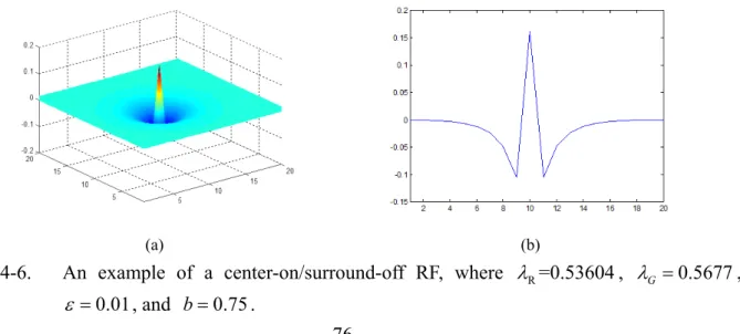
Figure 4-6. An example of a center-on/surround-off RF, where λ_R=0.53604, 0.5677λ_G = ,

0.01

ε = , and b=0.75. 76

Figure 4-7. An example of the model, where (a) is the input and (b) represents the output of the ganglions, while (c) shows the intensity of a section of (b). Notably, the behaviors of this model resembles that of the human vision visual system (see

Figure 4-3). 77

Figure 4-8. Another example of the proposed model, where the input is a natural image. (a) is the input, (b) is the output of the horizontal cells, (c) is the output of the ganglions, and finally, (d) is the output following the rectification. Notably, to present the structure of the hexagonal structure, the resolution of the image is

reduced in this example. 77

Figure 4-9. This study uses a red-green and a blue-yellow channel as the input of the center-red-on/surround-green-off and center-blue-on/surround-yellow-off ganglions, and consequently the new red-to-green and blue-to-yellow chromatic aberrations are obtained. (a) shows the test image and (b) illustrates the reconstructed result. These new chromatic aberrations were used to reconstruct the image, and compare it with the original. The average of Peak Signal to Noise Rate (PSNR) is 32.2263 (dB), while (c) shows the simulation result of the CRVO. 78 Figure 4-10. A case of a retinal injury and its visual response, where (a) demonstrates a

retina with Central Retinal Vein Occlusion (CRVO). The vein on the left side of the fovea is clogged and results retinal injury. (b) demonstrated that the patient will “sense” a piece of gray in the area of the retina that has lost blood circulation. 78 Figure 4-11. (a) represents the corresponding responses of the L-cone, the M-cone, and the

S-cone cells in the different wavelengths, (b) is the spectral power distributions of the RGB primaries, and (c) represents the transformation look-up table which describes nonlinear relationship between the frame-buffer values in the image data and the intensity of the light emitted by each of the primaries on the display,

named the Display Gamma Curve (DGC). 79

Figure 5-1. The diagram of proposed algorithm 99

Figure 5-2. An example which demonstrated coarse boundary detected by first order feature, where (a) input image, and (b) represents the boundaries has been extracted

from first order features. 99

Figure 5-3. An example which demonstrated the effect of first order feature in boundary detection. (a) is the input images which can be obtained from Brodatz texture database (D101-D102) [61], (b) represents the boundary has been detected by second order feature, and (c) represents the boundary has been detected by first

(13)

13

Figure 5-4. An example of 2D Gabor type filtering. (a) is a standard 2D Gabor type filter in

time domain, and (b) is in frequency domain. 100

Figure 5-5. An example of Gabor filter dictionary. (a) represents the Gabor-type filter bank set, and (b) is the Feature space of Gabor filter dictionary. 101 Figure 5-6. An example of proposed Gabor-type filtering. 101 Figure 5-7. An example demonstrates the effect of rectifying (a) input; (b) output without

rectifying; (c) output with rectifying 102

Figure 5-8. (a) input; (b) output before rectification; (c) output after rectification. 103 Figure 5-9. (a) is the input image, (b) is the coarse boundary, (c) is the 3D version of (b), (d)

is the results after peak detection. 103

Figure 5-10. The simulation results of proposed algorithm. 104 Figure 5-11. The example of dividing of the input images. 104 Figure 5-12. The implementation results of proposed algorithm. 105 Figure 5-13. An example of error estimation (a) input; (b) answer(middle line); (c) output; 105

Figure 5-14. Histogram of error estimation 106

Figure 5-15. An example of test image with big estimation errors(D50D32); (a) input; (b) output; 106 Figure 5-16. An example of test image with big estimation errors(D105D83); (a) input; (b)

output; 106 Figure 5-17. An example of test image with big estimation errors(D17D70); (a) input; (b)

output; 107 Figure 6-1. An example of improvement in image sharpness, where (a) is the input and (b)

shows the output. The images can be obtained at (http://cnn.cn.nctu.edu.tw/~chhuang/paper/hCNNCFM/). 121 Figure 6-2. Two results of the proposed image color constancy algorithm. First, a photo is

taken under a blue light condition. The photo is shown in (a), and the reconstructed result is shown in (b). Next, a photo is taken of the same scene under yellow light condition, as shown in (c), and the reconstructed result is shown in (d). The chromatic diagrams are shown to the side of the images. The

images can be obtained at (http://cnn.cn.nctu.edu.tw/~chhuang/paper/hCNNCFM/). 122

Figure 6-3. Two experimental results of the integrated video auto adjustment and enhancing algorithm, where(a), (c) are the input videos, (c) and (d) are the reconstructed outputs. The full video can be obtained at (http://cnn.cn.nctu.edu.tw/~chhuang/paper/hCNNCFM/). 123

Figure 6-4. The architecture of Neural PCA. 123

Figure 6-5. Texture example in this experiment. Here we have 32 images. From (a1) to (d4), some of those images is similar to each other expect the rotation effects. From (a5) to (d8), some of those images is similar to each other expect the scale

(14)

14

effects. 124 Figure 6-6. The eigenvalues in the proposed rotation-invariant texture classifier. 125 Figure 6-7. We plot the feature vectors of texture image in Figure 6-5 as sequences. The

feature vectors of Figure 6-5(a1), (b1), (c1), and (d1) have been shown in (a), and the feature vectors of Figure 6-5(a1), (a2), (a3), and (a4) have been shown

in (b). 125

Figure 6-8. The eigenvalues in the proposed Scale-invariant Texture Classifier. 125 Figure 6-9. We plot the feature vectors of texture image in Figure 6-5 as sequences. The

feature vectors of Figure 6-5(a5), (b5), (c5), and (d5) have been shown in (a), and the feature vectors of Figure 6-5(a5), (a6), (a7), and (a8) have been shown

in (b). 126

Figure 6-10. The architecture of SOFIN. 126

Figure 6-11. The architecture of the algorithm which has been proposed in this paper. The connection of Rule Layer will be generated after training stage finished. 127 Figure 6-12. The membership function of fuzzification and defuzzification in proposed

algorithm 127 Figure 6-13. The training patterns. The desired output for (a) is 0.75, for (b) is 0.25, for (c) is

-0.25, and for (d) is -0.75. 128

Figure 6-14. (a) is the testing pattern, (b) is the desired output, and (c) is the output of testing pattern. 128 Figure 6-15. The training pattern of a car plate segmentation. 129 Figure 6-16. The results of a car plate segmentation. 129

(15)

15

LIST OF TABLES

Table 4-1. Corresponding λ in Eq.(4-5) for deviation σ in Eq.(4-4). 80 Table 4-2. The result of Rotation-invariant Texture Classifier. The input texture images

have been shown in Figure 6-5. The rate of correct classification is about 97.5%. 80 Table 4-3. The result of Scale-invariant Texture Classifier. The input texture images have

(16)

16

1 INTRODUCTION

For decades, numerous scientists have examined the following questions: “How do humans see the world?” and “How do humans experience vision?” To answer these questions, this study proposes a Computer Visual System (CVS) based on the biological structure of Human Visual System (HVS). In this study, we focus on two major biological mechanisms, namely retina and cortex. Certain biological mechanisms of a retina can be simulated using an in-state-of-art architecture named Cellular Neural Network (CNN) since the simality between the biological neurons and the CNNs, and used some soft computing methods to simulate and evaluate the recognition methods for image textures in a HVS. The biological mechanisms include the behaviors of photoreceptors, horizontal cells, ganglions, and their co-operations.

As a highly structured neuron network, a retina extracts and processes the stimulation from an image projected upon it by the optical system of the eye [1-3]. This process is extremely complex. Consequently, analyzing, modeling, and even simulating the retina have been considered highly challenging tasks. To meet these challenges, numerous studies have been published during the past decade: for example, Shah et al. studied the information processing procedure of the retina in both the space and time domains [4]. Based on the study of Shah et al., Thiem later proposed a bio-inspired retina model capable of implementing some visual properties in the HVS [5]. Roska and Bálya et al. even discussed the parallel structure of retina and proposed an implementation on Cellular Neural Networks (CNNs) [6]. Their study demonstrated that certain visual information enhancing mechanisms exist in the HVS.

A visual cortex is the visual information processor of a human brain. The major parts exist on the upper and lower lips of calcarine sulcus on medical surface of cerebral hemisphere and provide simple texture recognition and association for the textures on an image.

(17)

17

The visual cortex is also able to effortlessly integrate the local features to construct our rich perception of patterns, despite the fact that the visual information is discretely sampled by the retina and the cortex. According to some biological and computational evidences, some kinds of data compression procedure occur at a very early stage in the HVS [2]. Moreover, many physiological evidences imply that some form of this compression mechanism is involved in the mechanism locating the boundaries in the image [7]. In the early 1960s, there was a research result which implied that the majority of neurons in the primary visual cortex respond to a line or a boundary of a certain orientation in a given position of the visual field [2]. In 1981s, Hubel and Wiesel found two types of orientation-selective neuron, one of that is sensitive to the areas of lines and boundaries, called simple cells, and the other is not, called complex cells [8]. The receptive field of the simple cells can be modeled by the Gabor function, and it has been widely used for information extraction, which is the so-called second order feature [7]. The mechanism of second order feature extraction is more commonly known as the filter-rectify-filter cascade. This consists of the early linear filtering subunits, a nonlinearity (e.g., rectification), and a late linear filter.

In this thesis, first the fundamental theories and the applications of the CNN are introduced and some new templates are developed. Next, the computer retina model is discussed. The relationships between the proposed model and a biological structure are presented. Even more, some applications are shown. Third, the computer cortex model is discussed. In this study, several methods are used to implement the proposed model and are followed by several applications. Finally, the conclusions are drawn.

(18)

18

2 FUNDAMENTAL THEORIES

Cellular Neural Network, also known as CNN, has already been proved as a very powerful image processing kernel with artificial intelligent abilities [9, 10]. Since Chua and Yang first introduced CNN, it has been widely applied on many areas. CNN is an alternative fully connected neural network and has evolved into a paradigm for this type of array. As shown in Figure 2-1(a), the dynamic equation of CNN can be represented by the following equation

( )

(

) ( )

( )

(

) ( )

( ) , , , , , , , ; , , , ; , , , r r t t t k l N i j k l N i j x i j x i j A i j k l y k l B i j k l u k l Z ∈ ∈ = − + + +

∑

(2-1) where

( )

1

(

1 1

)

2 t t t t y = f x = x + − x − , (2-2)

where Eq.(2-2) can be represented as Figure 2-1(b).

2.1 Stable Central Linear Systems and their Inverse Systems

If the CNN is considered as an image processor then numerous linear properties must be analyzed; for example, the states located in the non-saturated region. Crounse and Chua mentioned how to analyze the CNN-based image processing in the frequency domain [11]. A similar mechanism can be applied to the hexagonal-type CNN [12]. Assuming all of the cells operate in the linear region, that is, |x_i| 1< , then y_i =x_i. Thus, Eq.(2-1) can be reformulated as

( )

(

) ( )

( )

(

) ( )

( ) . t t t N N d x x A x dt B u Z ∈ ∈ = − + − + − +

∑

j i j i i i i j j i j j (2-3)

(19)

19

Let a_n∈A, the linearized templates then can be represented by [11]

( )

1, 0 , 0, otherwise r A a A N − = ⎧ ⎪ =_⎨ ∈ ⎪ ⎩ n n n n n i , and ,

( )

0, otherwise r B N b _{= ⎨}⎧ ∈ ⎩ n n n i . (2-4)

The dynamics can then be represented in a convoluted form as

( )

( ) ( )

( )

t t

d

x a x b u Z

dt n = n ⊗ n + n ⊗ n + , (2-5)

where ⊗ represents a hexagonal convolution. The dynamics can be written into [13]

( )

( ) ( )

( )

t

d

X A X B U Z

dt w = w w + w w + δ w , (2-6)

if and only if all of the discrete hexagonal Fourier transforms exist. Regarding the dynamics, assume that infinite time is available and that a discrete hexagonal Fourier transform exists for all

w, then Eq.(2-6) can be represented as follows [11]

( )

( ) ( )

X_∞ w =H w U w , (2-7) where

( )

B

_{( )}

( )

H A − = n n n . (2-8)

It is already known that if ( ) 0A w < for all w, then the central linear system will be stable. Thus, the equilibrium state can be thought of as a version of the input that has been spatially filtered by the hexagonal transfer function H w [14]. ( )

(20)

20

2.2 Implementing Existed Filters on the Cellular Neural Networks

This study realizes some operators that are required by the proposed model. These operators include CNN-based Laplace-like operators, CNN-based Gaussian-like operators and corresponding inverse operators. These operators are introduced in the following sections.

2.2.1 CNN-based Laplace-like Filtering

A Laplace operator can be represented as

( )

01 41 01 0 1 0 r l − ⎡ ⎤ ⎢ ⎥ = −_⎢ − _⎥ ⎢ − ⎥ ⎣ ⎦ n . (2-9)

The zero-frequency component of the Fourier transform of Eq.(2-9) is zero. This fact implies the inverse operation of Eq.(2-9) is difficult in the discrete environment. Thus, a small positive value

2

ε is added to Eq.(2-9). Accordingly, the Laplace-like operator is modified as follows

( )

2 0 1 0 1 4 1 0 1 0 r l ε − ⎡ ⎤ ⎢ ⎥ = −_⎢ + − _⎥ ⎢ − ⎥ ⎣ ⎦ n . (2-10)

Notably, the value of ε approaches zero as ( )l n approaches a Laplace operator. If and only _r

if the Fourier transform of the Laplace-like operator ( )l n exists and is denoted as

( )

{ }

l =L

( )

w n w

F . (2-11)

Next, map Eq.(2-11) into Eq.(2-8). Since ( ) 0A w < for all w is required, we choose ( )A w = −1. Thus

(21)

21

( )

1 B L L A − − = = − w w w w . (2-12)

According to Eq.(2-4), the coefficients of the system that has been described in Eq.(2-12) can be represented as

( )

a n = −δ n , and b

( ) ( )

n =l n . (2-13)

Thus, the templates are given by A a= ( )n +δ( )n , and B b= n , where ( )( ) δ ⋅ represents Dirac

Delta function. Finally, for the CNN-based Laplace-like operator, the templates are as follows

0 0 0 0 0 0 0 0 0 r A ⎡ ⎤ ⎢ ⎥ = ⎢ ⎥ ⎢ ⎥ ⎣ ⎦ , and 2 0 1 0 1 4 1 0 1 0 r B ε − ⎡ ⎤ ⎢ ⎥ = −_⎢ + − _⎥ ⎢ − ⎥ ⎣ ⎦ . (2-14)

For convenience, this study denotes the CNN-based Laplace-like operator is denoted as follows

( )

(

)

Laplace,

CNN ε u k , (2-15)

where ( )u k is the input, ε is a corresponding parameter, and the initial state of all cells is zero.

In fact, for any CNN, if the initial condition x , the template ₀ A , and the bias I are zero,

then the system is simply a FIR system and the template B can be considered as the FIR operator.

For the inverse Laplace-like operator, the inverse system of Eq.(2-12) can be used. That is

( )

1

( )

1 B L L A − − ₌ ₌ − − w w w w . (2-16)

(22)

22

Notably, since the condition, ( ) 0A w < for all w must be satisfied, this study sets

( ) ( )

A w = −L w . Thus, the templates can be obtained as following

(

2

)

0 1 0 1 3 1 0 1 0 r A ε ⎡ ⎤ ⎢ ⎥ =_⎢ − + _⎥ ⎢ ⎥ ⎣ ⎦ , and 0 0 0 0 1 0 0 0 0 r B ⎡ ⎤ ⎢ ⎥ = ⎢ ⎥ ⎢ ⎥ ⎣ ⎦ . (2-17)

For convenience, the CNN-based Inverse Laplace-like Operator is denoted here as follows

( )

(

)

1

Laplace,

CNN− _ε u _k _{, (2-18)}

where ( )u k denotes the input, and ε represents the corresponding parameter in Eq.(2-14). The initial condition x and the bias I are zero. ₀

2.2.2 CNN-based Gaussian-like Filtering

Kobayashi et al. suggested an active resister network for Gaussian-like filtering for image [11]. The

proposed system can be described as follows [14, 15]

( )

v

( )

_{( )}

h u = n n n , (2-19) where _u

( )

₌⎡₁ _{− +}

(

₂ _λ2

)

₁⎤ ⎣ ⎦ n , _v

( )

₌_⎡₀ ₋_λ2 ₀_⎤ ⎣ ⎦ n . (2-20)

The Fourier transforms are denoted as F { ( )}_w u n U( )w , and F { ( )}_w v n V( )w , then the system can be described as

( )

B

_{( )}

( )

V

( )

_{( )}

H U A − = w = w w w w . (2-21)

(23)

23 Thus, the templates can be obtained by

( ) ( )

A u= n +δ n , and B= − nv

( )

. (2-22)

The templates for different architectures are listed below

1-D CNN:

(

2

)

1 1 1 A=⎡_⎣ − +λ ⎤_{⎦ , and} _B _⎡₀ _λ2 ₀_⎤ = ⎣ ⎦ , (2-23) 2-D Rectangular-type CNN:

(

2

)

0 1 0 1 3 1 0 1 0 r A λ ⎡ ⎤ ⎢ ⎥ =_⎢ − + _⎥ ⎢ ⎥ ⎣ ⎦ , and 2 0 0 0 0 0 0 0 0 r B λ ⎡ ⎤ ⎢ ⎥ = ⎢ ⎥ ⎢ ⎥ ⎣ ⎦ , (2-24)

Shi proposed a CNN-based Gabor-type filtering model based on the study of Kobayashi [14]. His model is based on a Gaussian-like operator similar to Eq.(2-24) However, Shi modified the dynamic equation of the CNN to reduce the complexity of the hardware implementation. The proposed model requires no such modification.

For convenience, we denotes the CNN-based Gaussian-like operator as follows

( )

(

)

Gaussian,

CNN _λ u k , (2-25)

where ( )u k is the input, λ is the corresponding parameter, and the initial condition x and the ₀

bias I are zero.

(24)

24

( )

B

_{( )}

( )

U

_{( )}

( )

H V A − = w = w w w w . (2-26)

Since the condition ( ) 0V w < for all w must be met, it is concluded that ( )B w = −U( )w . The templates can be obtained from A v= ( )n +δ( )n and B= − n . u( )

The CNN-based inverse Gaussian-like operators for different architectures are listed as follows

1-D CNN: 2 0 1 0 A′ ⎡=_⎣ − +λ ⎤_{⎦ , and} _B_{′ = −}⎡₁ _{− +}

(

₂ _λ2

)

₁⎤ ⎣ ⎦ , (2-27) 2-D Rectangular-type CNN: 2 0 0 0 0 1 0 0 0 0 r A λ ⎡ ⎤ ⎢ ⎥ ′ =_⎢ − + _⎥ ⎢ ⎥ ⎣ ⎦ , and

(

2

)

0 1 0 1 4 1 0 1 0 r B λ ⎡ ⎤ ⎢ ⎥ ′ = −_⎢ − + _⎥ ⎢ ⎥ ⎣ ⎦ , (2-28)

Finally, a CNN-based inverse Gaussian-like operator can be denoted as

( )

(

)

1

Gaussian,

CNN− λ u k , (2-29)

where ( )u k denotes the input, λ represents the degree of Gaussian function and the initial condition x and the bias ₀ I are zero.

2.2.3 CNN-based Gabor-like Filtering

Gabor proposed an adaptive band-pass filtering method [16], which is a complex exponential function modulated by a Gaussian filter:

( )

( 2 2) 2 ( ) 0 0 2 1 , 2 x y x y j x y g x y e σ e ω ω πσ − + = , (2-30)

(25)

25

where ω_x₀ and ω_x₀ represent the angular frequency in x and y directions respectively, and σ

is the standard deviation of the Gaussian. The Gabor filter can be used as an adjustable band-pass filter tuned to frequencies near ω_x₀ and ω_x₀.

In 1998, Shi implemented Gabor-type filtering in space and time with CNNs [14]. According to Shi, a low-pass filtering modulating a complex exponential function will result in Gabor-type filtering. In Shi’s research, the following templates can be used to represent low-pass filtering in CNN:

(

2

)

0 1 0 1 4 1 0 1 0 A λ ⎡ ⎤ ⎢ ⎥ =_⎢ − − _⎥ ⎢ ⎥ ⎣ ⎦ , 2 0 0 0 0 0 0 0 0 B λ ⎡ ⎤ ⎢ ⎥ = ⎢ ⎥ ⎢ ⎥ ⎣ ⎦ , (2-31)

and the following equation can represent a low-pass filtering modulating a complex exponential function:

(

)

0 0 0 0 2 0 0 4 0 0 y x x y j j j j e A e e e ω ω ω ω λ − − ⎡ ⎤ ⎢ ⎥ = ⎢ − − ⎥ ⎢ ⎥ ⎢ ⎥ ⎣ ⎦ , 2 0 0 0 0 0 0 0 0 B λ ⎡ ⎤ ⎢ ⎥ = ⎢ ⎥ ⎢ ⎥ ⎣ ⎦ . (2-32)

Clearly, Shi’s CNN-based Gabor-type filter is orthogonal in the domain. This fact implies a problem since in hexagonal-type image processing, the sampled signals present non-orthogonal structure. Thus, the parameters,

0 x

ω and 0 y

ω , cannot be referred in hCNN-based Gabor-type filtering.

Here, a similar method can be used. The templates for different architectures are listed below

1-D CNN:

(

)

0 1 2 0 j j A′ =⎡_⎣eω − +λ e− ω ⎤_{⎦ , and} _B_{′ ⎡}₀ _λ2 ₀_⎤ = ⎣ ⎦ , (2-33)

(26)

26 2-D Rectangular-type CNN:

(

)

0 0 0 0 2 0 0 3 0 0 y x x y j j j r j e A e e e ω ω ω ω λ − − ⎡ ⎤ ⎢ ⎥ ′ = ⎢ − + ⎥ ⎢ ⎥ ⎢ ⎥ ⎣ ⎦ , and 2 0 0 0 0 0 0 0 0 r B λ ⎡ ⎤ ⎢ ⎥ ′ = ⎢ ⎥ ⎢ ⎥ ⎣ ⎦ , (2-34)

Finally, a CNN-based inverse Gabor-like operator can be denoted as

( )

(

)

0 0 1 Gabor, x , y CNN− _{ω ω} u _{k . (2-35)}

(27)

27

(a) (b)

(28)

28

3 HEXAGONAL-TYPE CELLULAR NEURAL NETWORK MODEL FOR PRELIMINARY VISUAL PROCESSING

CNNs are especially considered as image processors in many areas. Based on their flexibilities and artificial-intelligence-like abilities, CNNs provide extremely high performance. One of the flexibilities is that CNNs can be considered as one kind of parallel and symmetric structure neural network. Usually, CNNs are considered as eight-connected structure among one cell and its neighbor cells. In fact, CNNs cannot only be considered as eight-connected. If we consider constructing CNN on a flat plane, the cells can be connected as any kind of symmetric structure. One possible structure is six-connected structure, or as the well-known, the hexagonal-type structure.

In fact, constructing image as a hexagonal-type structure is not a new concept. In decades, many researches have examined various aspects of this issue. Peterson initiated the studies of hexagonal sampling [17]. According to Peterson, hexagonal sampling can be considered in the context of a possible alternative sampling regime for a two-dimension Euclidean space. Thus, he concluded that the most efficient sampling schemes were not based on rectangular-type, and same conclusions can explain why the distributions of the cells in the nature present hexagonal-type (see Figure 3-1). Moreover, Rosenfeld proposed distance functions on digital pictures using a variety of coordinate systems [18]. According to Rosenfeld, simple morphological operators were then evaluated in these coordinate systems via some simple applications. Finally, Rosenfeld had a suggestion for displaying the hexagonal-type images by staggering the individual square pixels like the bricks on a wall. The bricks are used to present pixels, and these pixels and their neighborhood construct the hexagonal-type structure. Based on this, Golay developed hexagonal-structured, parallel, computing systems. Other authors also studied the possibilities of using the hexagonal-type structures to represent digital images and graphics. The hexagonal-type structure is considered to be

(29)

29

superior to the rectangular-type system in many studies [19-26], and is even proved to be optimal in some applications [26-28].

The degree of symmetry in the hexagonal-type structure is higher than the rectangular-type structure. This fact results in a considerable saving of both storage and computation time [24, 29]. This property also enables the design of simple, accurate, local operators as compared with those currently used in rectangular-type systems. Hexagonal-type pixels are in a uniformly connected, close-packed form, so that greater angular resolution, higher efficiency, and better performance are achieved in many hexagonal-type models [19, 21, 24, 29].

There are some researches mentioned about type representation for CNNs. For example, Radványi (2000) indicates that the rectangular-type structure provides most flexible abilities [30]. However, in the area of image processing, following issues support in initialing the research of CNNs for Hexagonal Image Processing (HIP); first, according to Seiler and Nosse, the symmetry properties of image sampling should be considered. For example, the higher symmetry properties of the hexagonal type lead to a significant reduction in the complexity of the templates [31]. Second, in 1999s, Cauwenberghs and Waskiewicz proposed an analog VLSI focal plane implementation based on hexagonal-type neural networks [32]. In their study, choosing hexagonal-type structure can reduce the complexity of connection between the neighbor cells. Obviously, to consider the cost of connection neighbor cells, the performance of six-connected structure is higher than that of eight-connected one. Third, many studies in the area of image processing mentioned that hexagonal image processing has higher efficiency. According to Nel, the sampling efficiency of triangular-type structure is less than 60.46%, rectangular-type structure is less than 78.56%, and hexagonal-type structure is about 90.69% [33].

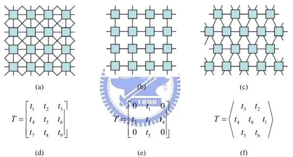
Figure 3-2 shows the comparison between different types of the architectures, where Figure 3-2(a), Figure 3-2(b), and Figure 3-2(c), are the 8-connected rectangular-type, the 4-connected

(30)

30

rectangular-type, and the 6-connected hexagonal-type CNN respectively, and Figure 3-2(d), Figure 3-2(e), and Figure 3-2(f) are their templates. We can see that in the 8-connected structure, there are some conflicts of connections in the diagonal directions of 8-connected rectangular-type CNN. That is a problem in hardware implementation (see Figure 3-3). This problem was solved based on the architecture of the 4-connected rectangular-type CNN. However, the abilities of the templates are limited. The 6-connected hexagonal-type CNN is not only has no confliction problems, but also has better performance.

Based on the above, we can say that to study the properties of hexagonal-type CNN structure, whichever linear or nonlinear regions, seems still an important issue. This issue leads us to study the field of CNN in hexagonal image processing. In this section, first, we introduce some background and the fundamental of proposed model. Next, the proposed architecture and related knowledge will be presented. Third, some simulations and experiments will be discussed. And finally, the conclusions follow.

3.1 Hexagonal-type Image Sampling Systems

Let x t_a

( )

be a 2D analog signal which represents the images, where t=

[

t₁ t₂

]

T, and s t

( )

be a 2D sampling signal and can be represented as follows

( )

(

)

1 - 2 -n n s ∞ ∞ δ = ∞ = ∞ =

∑ ∑

t t Rn , (3-1) where

[

1 2

]

T n n = n , and R=

[

r₁ r₂

]

. (3-2)

In Eq.(3-2), n represents an integer vector, R is the so-called sampling matrix, and δ

( )

⋅

(31)

31

is used to determine how the sampling system works. For example, let r and ₁ r be defined as ₂ follows 1 1 2 0 T ⎡ ⎤ = ⎢ ⎥ ⎣ ⎦ r , and 1 2 2 T T − ⎡ ⎤ = ⎢ ⎥ ⎣ ⎦ r . (3-3)

Note that T and ₁ T are related to the sampling period ₂ τ , and the type is hexagonal since each

sample location has exactly six nearest neighbors when the following equations stand

1 1 2

T = τ , and T₂ = 3T₁, (3-4)

where τ represents the sampling period of the sampling system. In fact, the distance between one sampling point and one of it’s six nearest neighbors equals to τ .

Let x n

[ ]

represent the discrete signal which is generated by the sampling system; it can be obtained by the following equation

( )

( ) ( )

s a x t =x t s t , (3-5) and

[ ]

s

( )

a

( )

x n x Rn =x Rn , (3-6)

where t=

[

t₁ t₂

]

T , R=

[

r₁ r₂

]

, n=

[

n₁ n₂

]

T, and x[ ]n is the discrete sampling signal.

3.2 Re-sampling Images from Rectangular-type to Hexagonal-type

In current display and sampling technology, digital images are usually sampled on rectangular-type structure. It is because sampling on a rectangular-type can be processed as the matrix, and it is

(32)

32

suitable for whenever calculating or computing. On the other hand, rectangular-type structure is easier to manufacture. However, we already realized that using hexagonal-type sampling provides several advantages [13, 24]. For example, a hexagon has a twelve-fold symmetry as compared to eight-fold of a square. Due to the improved packing density, hexagonal-type is better suited for representing isotropic and band limited signals. The higher degree of symmetry can also be used to design more isotropic filters to be applied on hexagonal-type [29, 34, 35]. The six neighbors of a hexagonal cell and their connectivity is well-defined [19] and has been used for better edge detection and pattern recognition.

Thus, reconstructing hexagonal-type images from rectangular-type images becomes a more important task. Fortunately, In 2004, Ville and his colleagues proposed a solution for this problem [36]. According to Ville, the image re-sampling between rectangular-type and hexagonal-type can be represented as following: first, an image in the continuous domain is reconstructed; second, resampling the image in the continuous domain based on the desire type.

To construct a spline bases in the hexagonal-type space, the following equations are used

( )

1 p 1

( )

p η η η ₌ ∗ − Ω x x , n≥1, (3-7)

where Ω = det

( )

R , where R is the so-called sampling matrix and has been defined in Eq.(3-2).

The signal can be represented as

( )

( ) ( )

( ) (

) ( )

( )

2 2 | ; n n S η =⎧_⎨s s = c η − c ∈l ⎫_⎬ ⎩

∑

k ⎭ x x k x Rk k Z , (3-8)

which means that each signal is characterized by its coefficient c k

( )

, which represents being discrete/continuous.

(33)

33

A common way to determine the spline coefficient c k

( )

is to impose the interpolating condition, s

( )

Rk =g

( )

Rk at the sampling points, where g x

( )

is the original signal we choose to represent using the splines.

3.3 Hexagonal-type Discrete Fourier Transform

Let x t_a

( )

be the 2D analog signal which represent the images, where t=

[

t₁ t₂

]

T , and s t

( )

is 2D hexagonal-type sampling signal and can be represented as follows

( )

{

( )

}

( )

( ) ( )

( )

(

)

( ) (

)

(

)

( )

(

)

1 2 1 2 1 2 1 2 1 2 1 2 1 2 1 2 T T T T T j s s s j a j a n n j a n n j a n n X j F x x e dt dt x s e dt dt x e dt dt x e dt dt x e dt dt δ δ δ ∞ ∞ − Ω −∞ −∞ ∞ ∞ − Ω −∞ −∞ ∞ ∞ _∞ _∞ − Ω =−∞ =−∞ −∞ −∞ ∞ ∞ ∞ ∞ − Ω =−∞ =−∞ −∞ −∞ ∞ ∞ ∞ − Ω = =−∞ _{−∞ −∞} Ω = = = ⎛ ⎞ = _⎜ − _⎟ ⎝ ⎠ = − ⎛ ⎞ = _⎜ − _⎟ ⎝ ⎠

∫ ∫

∑ ∑

∫ ∫

∑ ∑

∫ ∫

∑

∫ ∫

t t Rn Rn t t t t t t Rn Rn t Rn Rn t Rn t

( )

[ ]

1 2 1 2 , T T j j a n n n n x e x e ∞ −∞ ∞ ∞ ∞ ∞ − Ω − Ω =−∞ =−∞ =−∞ =−∞ = =

∑

∑ ∑

_Rn Rn

∑ ∑

_n Rn (3-9) where t=

[

t₁ t₂

]

T , R=

[

r₁ r₂

]

, and n=

[

n₁ n₂

]

T.

According to Eq.(3-6), and let Ω =ω_τ , where τ is the hexagonal-type sampling period, the hexagonal-type discrete Fourier transformation can be obtained as follows

( )

{ }

[ ]

(

[ ]

)

1 2 T j j s n n X e F x ∞ ∞ x e− =−∞ =−∞ = _n =

∑ ∑

_n n ω ω _{, (3-10)}

(34)

34

can be obtained by the hexagonal-type Fourier transform of x t_a

( )

, X_a

( )

jΩ . According to Mersereau [37], Eq.(3-10) can be represented as follows

( )

(

( )

(

)

1 2 1 1 2 det T j s a n n X e ∞ ∞ X j − π =−∞ =−∞ =

∑ ∑

− ω _R _ω _n R , (3-11) where

( )

_j T a a X j x e d ∞ − Ω −∞ =

_∫

t Ω t t. (3-12)

Clearly, the inverse hexagonal-type discrete Fourier transformation can be represented as following

[ ]

{

( )

}

( )

-1 1 2 2 1 2 T j j j s s x F X e X e e d d π π π π ω ω π − − = ω =

∫ ∫

ω ω n n , (3-13) where ω=

[

ω ω₁ ₂

]

T and n=

[

n₁ n₂

]

T.

3.4 Hexagonal-type Image Indexing Scheme

In the previous session, we introduced sampling methodology in hexagonal-type image processing. Although the hexagonal-type image processing is more similar to biological phenomenon and it provides more compact structure [5]. The one of disadvantage is that there is no orthogonal axis in hexagonal-type images. Consequently, the mathematical processing in hexagonal-type image processing becomes a difficult task. Fortunately, Middleton and Jayanthi (2001) proposed his research which provides a scheme named Hexagonal Image Processing (HIP) Frameworks [38]. In HIP, the indexing scheme can be constructed intuitively by using an analog based upon tiling the image. Consider a single hexagon to be a tile at layer 0. This can then be surrounded moving anti-clockwise by a further 6 hexagons. This new structure forms a tile at layer 1, with the new tile

(35)

35

being the super-tile of layer 0. Similarly, this process can be extended to any number of layers. An example of layer 2 is illustrated in Figure 3-4. The number of hexagons that are contained in a given layer λ super-tile are 7λ. Each hexagon can then be numbered uniquely as a sequence of numbers where every digit gives its position in a given tile. The highlighted hexagon in Figure 3-1 is in the fourth tile in layer 2 and the second tile at layer 1. Thus, all the hexagons in a layer λ super-tile can be addressed uniquely by a λ-digit base 7 number. As previously stated, this number encodes spatial location, and as such, the number can be viewed analogously to a vector. This vector property can be used to define various arithmetic operations such as hexagonal addition and hexagonal multiplication [38].

Since convolution is more computationally efficient when computed in frequency domain, developing the Fourier transformation becomes an important task. There are several methods that can be used to implement Fourier transformation on the hexagonal image. Middleton and Jayanthi proposed their study which is based on Cooley-Turkey algorithm [13, 39]. In their research, the 3-coordinate system was chosen for Discrete Time Fourier Transform in HIP [40]. In this system, a function c

( )

⋅ is defined that converts from the single index to the 3-coordinate system which has been proposed by Her [40]. For this purpose, the pair of functions is defined as follows

( )

1

( )

1 1 1 2 1 1 2 1 3 j j j h g λ N ₋ c g = − ⎡ ⎤ = _⎢ _⎥ − − ⎣ ⎦

∑

, (3-14) and

( )

1

( )

1 1 2 1 1 2 1 1 3 T j j j H g λ N ₋ c g = − − ⎡ ⎤ = _⎢ _⎥ − − ⎣ ⎦

∑

, (3-15)

where g is a λ-level index, g corresponds to the j-th digit of the index, and _j N_j₋₁ is equivalent to _Nj−1_{. Base on those and the previous section, the discrete Fourier transformation for HIP} framework can be developed as follows

(36)

36

( )

₂ ( )T 1( ) jH k N h g k G x g X k e λ λ π − ∈ =

∑

. (3-16)

And the inverse function is

( )

₂ ( )T 1 ( ) jH k N h g g G X k x g e λ λ π − − ∈ =

∑

. (3-17)

3.5 Cellular Neural Networks for Hexagonal Image Processing

In this section, we focus on Hexagonal-type Cellular Neural Network (hCNN). hCNN can be represented as follows

(

) ( )

( )

(

) ( )

( ) ; ; , r r t t t h N g h N g x x A h g y h B h g u h I ∈ ∈ = − + + +

∑

(3-18)

( )

1

(

1 1

)

2 t t t t y = f x = x + − x − , (3-19)

where g and h represent the index in hexagonal image. Basically, Eq.(3-18) is a special case of Eq.(2-1).

For convenience, we use the following mathematical symbols to present the templates in hCNN 3 2 4 0 1 5 6 a a A a a a a a = , 3 2 4 0 1 5 6 b b B b b b b b = , and I = (3-20) z,

where A is the feedback template, B is the control template, and I is the bias. Note that the

(37)

37

3.5.1 The hCNN Stable Central Linear Systems

If we consider the CNN as an image processor, then many properties of the states which have been located in the non-saturated region will need to be analyzed. Crounse and Chua mentioned how to analyze CNN-based image processing in frequency domain. The similar mechanism can be applied on hexagonal-type CNN [11]. Assume the cells operate in the linear region. That is, x_g < , then 1

g g

y =x . Thus, Eq.(3-18) can be reformulated as follows

(

) ( )

( )

(

) ( )

( ) ; ; , r r t t t h N g h N g x x A h g x h B h g u h I ∈ ∈ = − + + +

∑

(3-21)

Assume a_n∈ , and the notation can be shifted so that spatial indices are written as A

arguments and time as a subscript. The linearized template can be represented as follows

( )

0

( )

1, 0 , 0, otherwise, h r a h a h a h N g − = ⎧ ⎪ =_⎨ ∈ ⎪ ⎩ and

( )

,

( )

0 otherwise. h r B h N g b h _{= ⎨}⎧⎪ ∈ ⎪⎩ (3-22)

Then the dynamics can be presented in convolution form as follows

( )

( ) ( ) ( )

t t

d

x g a g x g b g u g I

dt = ⊗ + + , (3-23)

(38)

38

Assume all of the discrete hexagonal Fourier transformations exist. The dynamics can be written into the following

( )

( ) ( )

( )

. t

d

X A X B U I

dt ω = ω ω + ω ω + δ ω (3-24)

For the dynamics, assume the time goes to infinite and all of the discrete hexagonal Fourier transformations exist, then it can be represents as follows

( )

( ) ( )

, X_∞ ω =H ω U ω where

( )

B

_{( )}

( )

H A ω ω ω − = . (3-25)

We already know that if A

( )

ω <0 for all ω, then the central linear system will be stable. Thus, the equilibrium state can be thought of as a version of the input that has been spatially filtered by the hexagonal transfer function H

( )

ω .

3.5.2 Implement hexagonal-type CNN on rectangular-type CNN

Since rectangular-type eight-connected CNN structure can provide most efficient flexibility [30], most CNN technology currently is based on this structure. This fact implies that we can implement hexagonal-type CNN by current technology. However, there are some fundamental different between rectangular-type eight-connected CNNs and hexagonal-type six-connected CNNs. Hence, some extra processing is required.

In this section, we propose two ways which can be considered to implement hexagonal-type six-connected CNN on a rectangular-type eight-connected CNN: one is image-rotated method;

(39)

39

another is image-expended method. Those two methods will be introduced as the following sections.

3.5.2.1 Image-screwed Method

According to Radványi, the hexagonal-type structure can be implemented quite easily by rectangular-type eight-connected CNNs, since the connection of neighbor cells can be reconnected based on graph theories [30]. In the case of hexagonal-type CNNs, the templates can be referred as

2 1 3 0 6 4 5 0 0 a a A a a a a a ⎡ ⎤ ⎢ ⎥ = ⎢ ⎥ ⎢ ⎥ ⎣ ⎦ , 2 1 3 0 6 4 5 0 0 b b B b b b b b ⎡ ⎤ ⎢ ⎥ = ⎢ ⎥ ⎢ ⎥ ⎣ ⎦ , and I = . (3-26) z

Clearly, the input and initial-state images of the CNNs should rotate 1

4π . The relationship between the templates and the images can be represented as Figure 3-5.

This method seems quite efficient. The cost is that the input and initial-state images are about twice size and pre-processing, which is used to rotate the input and initial-state image, has been required. However, considering the complexity of image rotating algorithm, realizing this method becomes very difficult. Moreover, this method will waste huge amount of memory if we use general CNN-UM.

3.5.2.2 Image-expended Method

If the 5×5 CNN array is available, and the buffer size of CNN array is big enough, then this method should be considered. Based on the requirement of symmetric property, the hexagonal-type CNN can be implemented by the following 5×5 templates

(40)

40 3 2 4 0 1 5 6 0 0 0 0 0 0 0 0 0 0 0 0 0 0 0 0 0 0 a a A a a a a a ⎡ ⎤ ⎢ ⎥ ⎢ ⎥ ⎢ ⎥ = ⎢ ⎥ ⎢ ⎥ ⎢ ⎥ ⎣ ⎦ , 3 2 4 0 1 5 6 0 0 0 0 0 0 0 0 0 0 0 0 0 0 0 0 0 0 b b B b b b b b ⎡ ⎤ ⎢ ⎥ ⎢ ⎥ ⎢ ⎥ = ⎢ ⎥ ⎢ ⎥ ⎢ ⎥ ⎣ ⎦ , Z = . (3-27) z

Obviously, the input and initial state images I can be reconstructed as follows

0,0 0,1 0, 1,0 1,1 1, ,0 ,1 , 0 0 0 0 0 0 0 0 0 0 0 0 0 0 0 0 0 0 0 0 0 0 0 0 0 0 0 N N M M M N p p p p p p I p p p ⎡ ⎤ ⎢ ⎥ ⎢ ⎥ ⎢ ⎥ ⎢ ⎥ = ⎢ ⎥ ⎢ ⎥ ⎢ ⎥ ⎢ ⎥ ⎢ ⎥ ⎣ ⎦ , (3-28)

where p represents the intensity of pixel in specific location _{i j}_,

( )

,i j in the hexagonal images. Clearly, since the template which has been described in Eq.(3-27) is fully symmetric in all direction, the output and state images also can be described as Eq.(3-28). That means after the iteration of CNN converged, the output images also should be reconstructed.

In this method, we can see that the 5×5 templates are required, and the size of CNN array is about 4 times of the size of input and initial-state images. It seems the cost of this method is higher than the previous one. However, considering the complexity of the pixel relocating algorithm, the image-expended method might be the better choice.

Based on the proposed architecture, a hexagonal image sampling method has been required. There are several methods can be applied on the proposed architecture. Consider the balance between the complex computation and the precise in geometry. We choose a method as shown in Figure 3-6 and it can be represented as following

(41)

41

( ) ( )

, , | if y and if y , , 2 2 , x y ∈⎧_⎨ x y x∈ ∈ x∈ ∈ y∈ ⎫_⎬ ⎩ ⎭ + = E E O O E E O R (3-29)

where E represents the domain of evens, and O represents the domain of odds in the domain of real numbers R .

However, assume every sampling pixel is perfect square, then the geometrical relationship among pixels can be represented as Figure 3-7. As we can see, the sampling rate will not be consistent in different direction. The error of distance between different directions is about 11.8%. Even so, the phenomenon can be compensated if we made the sampling rate of vertical direction higher than the horizontal direction. For example, we can make the sampling rate on vertical direction equal to 2 3 times of horizontal direction.

3.5.3 Hexagonal Image Presentation

Currently, implementing hexagonal-type structure in a rectangular display system is not an easy task. In our simulations, we used multiple pixels to present a hexagonal-type. On the other words, the rectangular display system, such as a computer monitor, has been considered as a digital signal sampling processor, and the resolution of the sampling processor is higher than the signals we processed.

Most of current image display technologies use rectangular-type for ease of calculation or presentation of the image. In order to represent an image described by the hexagonal-type, we used pseudo hexagonal pixel in the experiments. The pseudo hexagonal pixel is composed of small rectangular pixel which is widely used in current display technology as shown in Figure 3-8. With this representation, the aspect ratio of an image changes from 1:1 to 1:1.17.

We can compare the results between the image reconstructions by hexagonal-type pixels and by rectangular-type pixels. An image of plate has been shown in Figure 3-9. We can see that the

基於細胞神經網路的仿生型電腦視覺系統

基於細胞神經網路的仿生型電腦視覺系統

Bionic Computer Visual System

based on

Cellular Neural Networks

研 究 生：黃朝暉 Student：Chao-Hui Huang

指導教授：林進燈 博士 Advisor：Dr. Chin-Teng Lin

國 立 交 通 大 學

電 機 與 控 制 工 程 學 系

博 士 論 文

A Dissertation

Submitted to Department of Electrical and Control Engineering

College of Electrical Engineering and Computer Science

National Chiao-Tung University

in partial Fulfillment of the Requirements

for the Degree of

Doctor of Philosophy

in

Electrical and Control Engineering

June 2007

Hsinchu, Taiwan

基於細胞神經網路的仿生型電腦視覺系統

學生：黃朝暉 指導教授：林進燈

國立交通大學電機與控制工程學系﹙研究所﹚博士班

摘 要

Bionic Computer Visual System based on Cellular Neural Networks

Student：Chao-Hui Huang Advisors：Dr. Chin-Teng Lin

Department of Electrical and Control Engineering

National Chiao Tung University

ABSTRACT

ACKNOWLEDGEMENTS

CONTENTS

LIST OF FIGURES

LIST OF TABLES

( )

( )

(

) ( )

(

) ( )

∑

∑

( )

(

)

( )

( )

(

) ( )

(

) ( )

∑

∑

( )

( )

( )

( )

( )

( ) ( )

( )

( )

( ) ( )

( ) ( )

( )

( )

( ) ( )

( )

( )

( )

( )

( )

( )

{ }

( )

( )

( )

( )

( )

( )

( )

研究生：黃朝暉 Student：Chao-Hui Huang

指導教授：林進燈博士 Advisor：Dr. Chin-Teng Lin

國立交通大學

電機與控制工程學系

博士論文

學生：黃朝暉指導教授：林進燈

摘要

_{( )}

_{( )}

_{( )}

_{( )}

_{( )}

_{( )}