行政院國家科學委員會專題研究計畫 期中進度報告
地下水徑向雙層微水試驗之閉合解(1/2)
計畫類別: 個別型計畫 計畫編號: NSC91-2211-E-009-020-執行期間: 91 年 08 月 01 日至 92 年 07 月 31 日 執行單位: 國立交通大學環境工程研究所 計畫主持人: 葉弘德 報告類型: 精簡報告 處理方式: 本計畫可公開查詢中
華
民
國 92 年 5 月 26 日
行政院國家科學委員會補助專題研究計畫
□ 成 果 報
告 ■ 期
中進度
報
告
地下水徑向雙層微水試驗之閉合解(1/2)
計畫類別:■ 個別型計畫
□ 整合型計畫
計畫編號:NSC - 91 - 2211 - E - 009 - 020
執行期間: 91 年 08 月 01 日至 93 年 07 月 31 日
計畫主持人:葉弘德
共同主持人:楊紹洋
計畫參與人員:
成果報告類型(依經費核定清單規定繳交):□精簡報告 ■完整
報告
本成果報告包括以下應繳交之附件:
□赴國外出差或研習心得報告一份
□赴大陸地區出差或研習心得報告一份
□出席國際學術會議心得報告及發表之論文各一份
□國際合作研究計畫國外研究報告書一份
處理方式:除產學合作研究計畫、提升產業技術及人才培育研究
計畫、列管計畫及下列情形者外,得立即公開查詢
□涉及專利或其他智慧財產權,□一年■二年後可公開
查詢
執行單位:國立交通大學
中文摘要
關鍵詞:微水試驗、徑向雙層、閉合解、部份貫穿井 微水試驗是將少量的水瞬間注入井中或從井中提出,同時記錄水位對時間的變化,再利 用測得數據分析含水層的水文地質參數。此方法的優點包括,施測簡單、快速、所需費用低 廉、及擾動到現地地下水位和污染分佈十分輕微,故目前被工程界廣泛應用於場址特性調查。 由於鑿井過程、完井、或現地地質非均質,含水層的水文地質特性,於井孔周圍可能會有異 質的現象,即含水層的水力傳導係數或/及蓄水係數值,較試驗井緣附近水層高或低,則此含 水層可視為一個徑向雙層系統(radial two-layered system)。若忽略此異質現象,視水層為一均 質系統,貿然進行微水試驗數據分析,會高估或低估含水層的水文地質參數值。又一般地下 水試驗井或水質監測井,濾管部分大都未全部貫穿水層。沒考慮此水井部份貫穿問題進行數 據分析,其結果可能會有顯著的誤差。本研究第一年計畫(進行中)工作,係針對完全貫穿受壓含水層之徑向雙層水流方程式, 利用 Laplace 逆轉換和 Bromwich contour 積分,推導一個新的時間域閉合解,目前我們已導 得該閉合解,並利用一個有效率的數值方法,估算此閉合解的數值。利用這個閉合解,可繪 製類似 Theis 方法的標準曲線,以利工程應用;此外,針對井膚層的厚度及特性,可量化分 析微水試驗時水層參數對水力水頭在時空上分佈的影響。
第二年(本年度)計畫,擬考慮水井部份貫穿的情況,利用 Laplace 轉換和 finite cosine 轉 換,以推導徑向雙層水流方程式的 Laplace 域水層水頭半解析解,再利用 finite cosine 逆轉換, 可求得水層水力水頭和井緣流量的 Laplace 域解,此解可用來探討井膚層和部份貫穿井兩者 的效應,對微水試驗數據分析的影響。
Abstr act
Keywords:slug test, radial two-layer aquifer, closed-form solution, partial penetration
The slug test is to suddenly remove/add a volume of water from/to a well, and the rate of fall/rise of the wellbore water level is simultaneously measured. The aquifer parameters, the hydraulic conductivity and the storage coefficient, can then be estimated based on the measured data. The slug test is widely used in aquifer site characterization because of the advantages of low cost, being easy and rapid to perform the test, and minor disturbances of the groundwater level and exiting contamination plume. The aquifer characteristics near the well may become higher or lower than those of the formation due to the well drilling process or the field heterogeneity. This may lead to over-estimate or under-estimate the slug-test results, if the aquifer well skin or heterogeneity is presented. Besides, the test well or monitoring well is very likely to be partially penetrated in the real world. The aquifer parameters obtained by analyzing the test data may also lead to significant errors while neglecting the effect of partial penetration.
In the first year of this study, we had derived a new closed-form solution for the change of water level by a slug test in a radial two-layer confined aquifer system. The methods of Laplace transform and the Bromwich contour integration were employed to solve the two-layered groundwater flow equation. In the near future, we will use this new analytical solution to generate a set of type curves for engineering application as well as to quantify the effects of different thickness of wellbore skin and aquifer characteristics on the hydraulic head distribution.
This year (the second year) we will derive the closed-form solution for a radial two-layer groundwater flow equation with considering the condition that the well is partially penetrated. The methods of Laplace transforms and finite cosine transforms may be employed to solve the two-layered groundwater flow equation with the appropriate initial and boundary conditions including the effect of the well partial penetration. The derived solution will be employed to investigate the effects of the wellbore skin and the partial penetration on the water level distribution
Table of Contents
Page
中文摘要 I
Abstract II
Table of Contents III
List of Tables IV List of Figures V 1. Introduction 1 2. Mathematical Derivations 3 2.1 Mathematical statement 3 2.2 Closed-form solution 4 2.3 Dimensionless 5 3. Verification of Solutions 8 4. Discussions 9
4.1 Effect of Skin Type 9
4.2 Effect of finite thickness skin 9
4.3 Effect of different skin thickness 9
4.4 Effect of Contrast of Transmissivity 10
5. Conclusions 11
References 12
計畫成果自評 26
List of Tables
Table Page
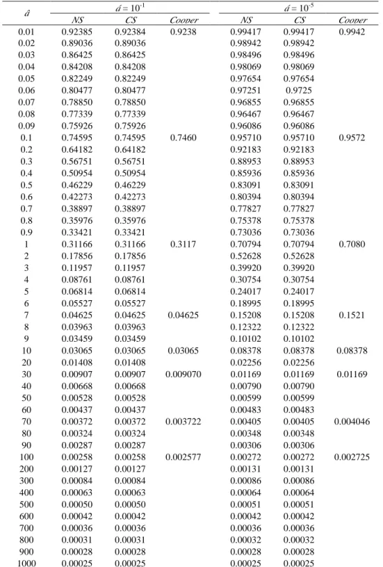
1 Dimensionless hydraulic head versus dimensionless time (â) estimated by the
closed-form solution, the numerical inversion from the Laplace-domain solution, and the one given in Cooper et al. (1967) for rDc = 0.5, rD = 1, rDs =
10, and ζ = ç = 1 while α = 10-1 or 10-5.
List of Figur es
Figure Page
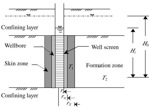
1 Schematic diagram of the well and aquifer configurations. 15
2 plots of dimensionless hydraulic head versus dimensionless time for rDs = 5, á
= 10-5, and â = 10-4 to 10 when (a) ζ = 0.1, (b) ζ = 1, and (c) ζ = 10.
16
3 A plot of dimensionless hydraulic head versus dimensionless time for rDc =
0.5, rD = 1, rDs = 10, ç = 1 and ζ = 0.1 when α ranged from 10-1 to 10-5.
19
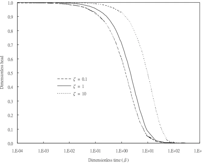
4 A plot of dimensionless hydraulic head versus dimensionless time for rDc =
0.5, rD = 1, rDs = 10, ç = 1, and ζ = 0.1, 1, and 10 when (a) α = 10-1 and
(b) α = 10-5.
21
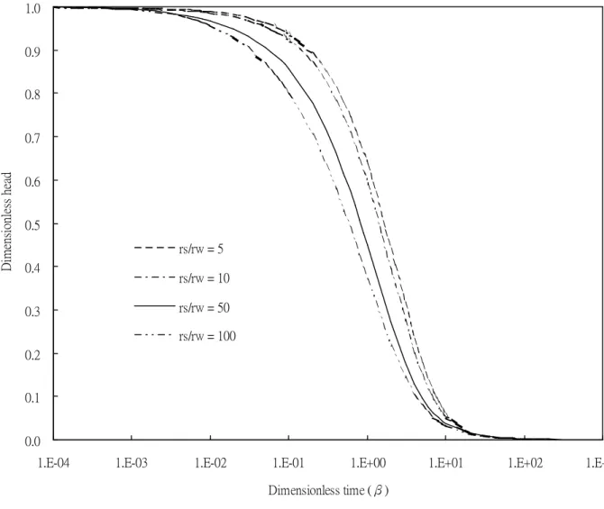
5 A plot of dimensionless hydraulic head versus dimensionless time for rDc =
0.5, rD = 1, α = 10-5, ç = 1, and rDs = 5, 10, 50, and 100 when (a) ζ = 0.1
and (b) ζ = 10.
23
6 A plot of dimensionless well water level versus dimensionless time for rDs =
10 and á = 10-1 and 10-5 whenζ = 0.1, 1, or 10.
25
A A plot of the closed contour integration of h for the Bromwich integral (Hildebrand, 1976).
28
1. Intr oduction
Slug test is one of the well-test methods to investigate in-situ aquifer parameters. The test involves an instantaneous removal/injection of a small volume of water from/into a well (Butler, 1997). An instantaneous head change is thus imposed within a well and the recovery/falloff of water level is continuously measured using a pressure transducer that connects to a data logger. The aquifer parameters, e.g., transmissivity and storativity, can then be obtained if the slug-test data is analyzed.
Ferris and Knowles (1954) originally introduced the slug-test data analysis procedure in a ground-water literature. They derived an approximated solution for describing the water level change of test well. The transmissivity is then estimated based on the straight line which represents residual head versus inverse of time. Bredehoeft et al. (1966), employing an electrical analog model of the well-aquifer system, demonstrated that Ferris and Knowles’ approximation is valid only for very late time of the test. Later, Cooper et al. (1967) obtained a solution including the well storage from being analogous to a heat conduction problem provided by Carslaw
for estimating aquifer parameters from the slug-test data. However, the aquifer parameters obtained by this technique may be very rough because the shape of type curve is rather insensitive to the value of aquifer storage S (Lohman, 1972), especially,
when S is very small. Kipp (1985) constructed a set of type curves that enables the
well water level response data from slug tests to be analyzed if the inertial parameter is large. Pandit and Miner (1986) provided an automatic fitting procedure to determine the aquifer parameters of transmissivity and storativity while analyzing the slug-test data obtained from a confined aquifer. Marschall and Barczewski (1989) presented an analysis of slug tests in the frequency domain for evaluating the solution of Cooper et al. (1967). The solution is in terms of the Kelvin functions, and the slug-test data is transformed by the numerical Fourier transforms to determine aquifer parameters. Such an approach can avoid evaluating the integrand, which is an oscillatory function and difficult to evaluate.
Using the infinitesimally thin skin concept, Ramey and Agarwal (1972) originally reported an analytical solution in terms of an inversion integral to the problem and its short-time and long-time approximating forms. The skin effect describing the damage or improvement to the region surrounding the well is represented by a skin factor. Ramey et al. (1975) presented the semilog and double-log type curves combined the effects of the well storage and the wellbore skin for analyzing the slug-test data. They provided a new correlation of type curves, which the dimensionless storage constants and times were based on the effective well radius determined with the skin effect. Their approach can overcome the difficulty in obtaining a unique solution when the skin presents. Faust and Mercer (1984) provided an infinite-aquifer solution to investigate the effect of a finite-thickness skin on the response of slug tests. They assumed that the skin has a much lower permeability than that of the adjacent formation. Under this condition, the skin effect can lead to very low estimates of hydraulic conductivity when using the type-curve fitting method of Cooper et al. (1967). Moench and Hsieh (1985) commented on the evaluation of slug tests in a finite-thickness skin by Faust and Mercer (1984). They showed that when the specific storage of skin is negligibly small, the finite-thickness skin solution becomes equivalent to the infinitesimally thin skin solution. Under a finite-thickness skin condition, the skin properties control the early time response, whereas the formation properties relate to the late time response. Further, Sageev (1986) investigated the effects of the well storage and the wellbore skin in a confined aquifer system. He obtained a similar result of Moench and Hsieh (1985). Various models of slug tests are attempted to develop solutions by Karasaki et al. (1988) for the linear flow, radial flow with boundaries, two layer, and concentric composite systems. They provided type curves for each solution and noted that slug tests suffer the problems of the non-uniqueness in matching the test data to type
curves. Butler and Healey (1998) investigated the estimate of hydraulic conductivity obtained through pumping or slug tests. They indicated that the hydraulic conductivity estimate from a pumping test is, on average, larger than that from a series of slug test in the same formation.
An aquifer is considered as a radial composite aquifer if the formation properties near the well are significantly changed due to the well drilling or development. The well drilling makes the invasion of drilling mud into the aquifer and may produce a positive wellbore skin that has lower permeability than that of the original formation. On the other hand, the extensive well development and/or substantial spalling and fracturing of the borehole wall may increase the permeability of the adjacent formation around the well. Under such circumstances, the disturbed formation is referred to as a negative wellbore skin. Karasaki (1990) presented a Laplace-domain solution of the well response to a drillstem test with the presence of skin. He used a convolution method to evaluate the solution numerically for converging the integration of functions. The systematized procedure and analysis method were proposed for a drillstem test. Recently, Yang and Gates (1997) constructed a numerical model in a confined aquifer considering the effect of a finite-thickness skin for slug test. The wellbore skin effect on the slug-test results was analyzed by using a finite-element method. They suggested that the effect of a wellbore skin on the estimates of hydraulic conductivity for low-permeability mediums could be minimized by the use of the late-time data.
The purpose of this paper is to derive a new closed-form solution in terms of hydraulic head distribution for slug tests performed in a radial confined composite aquifer. The governing equation and the related boundary conditions modeling the distribution of hydraulic head are solved by the Laplace transforms. This time-domain solution is expressed in terms of an integral that covers a range from zero to infinity and has an integrand consisting of complicate products terms of the Bessel functions. The closed-form solution is evaluated by numerical approaches. Its values are compared with those of Cooper et al.’s single-layer solution (1967) when the medium is uniform and the results of numerical inversion from the Laplace-domain solution. The derived solution for the hydraulic distribution can be used as a tool to investigate the effects of a finite-thickness skin, e.g., skin properties and skin thickness.
2. Mathematical Der ivations
2.1 Mathematical statement
Figure 1 shows the well and aquifer configurations for a two-layer confined aquifer system. The assumptions made for the solution of hydraulic heads are: (1) the aquifer is homogeneous, isotropic, infinite-extent, and with a constant thickness, (2) the well is fully penetrating with a finite radius, (3) the initial head is constant and uniform throughout the whole aquifer, and (4) vertical flow gradients are negligible. Under these assumptions, the governing equations for the skin region and the undisturbed formation can be written as
s w r r r t h T S r h r r h ≤ ≤ ∂ ∂ = ∂ ∂ + ∂ ∂ , 1 1 1 1 1 2 1 2 (1) and ∞ ≤ ≤ ∂ ∂ = ∂ ∂ + ∂ ∂ r r t h T S r h r r h s , 1 2 2 2 2 2 2 2 (2) where the subscripts 1 and 2 respectively represent the wellbore skin and undisturbed formation, r is the radial distance from the centerline of the well, rw is the radius of
the well, rs is the radius of the skin, t is the time from the start of the test, S is the
storage coefficient of the aquifer, T is the transmissivity of the aquifer, and h defined
as the dimensionless hydraulic head is
( ) i t H H H H h − − = 0 0 (3)
where H0 is the hydraulic head at ambient conditions, Hi is the head at time zero, and H(t) is the head at time t.
The dimensionless hydraulic head is initially assumed to be zero in both the skin and the undisturbed formation, that is
( )
r h( )
r r rwh1 ,0 = 2 ,0 =0, > (4) The initial condition for the wellbore is
(
,0)
11
r
w =h
(5) The dimensionless hydraulic head tends to zero, as r→ ∞, that is( )
, 02 ∞ t =
h (6) The conservation of mass requires that
( )
w r r w c r h T r t t H r = ∂ ∂ = ∂ ∂ 1 1 2 2π π (7)continuous,
( )
, 2( )
, , 01 r t =h r t t >
h s s (8) and there is conservation of mass:
( )
, 2( )
, , 0 2 1 1 > ∂ ∂ = ∂ ∂t
r
t
r
h
T
r
t
r
h
T
s s (9) 2.2 Closed-for m solutionThe dimensionless hydraulic head in the Laplace domain for the skin and the undisturbed formation can be obtained by using Laplace transform for (1) – (9). The results for h1 and h2 are respectively expressed as
( )
( )
(
)
(
)
[
]
[
(
)
(
)
]
′ + + ′ + − ′ + ′ − = 2 1 1 1 0 1 1 1 1 1 0 1 1 0 2 1 0 1 1 1 2 0 1 2 2α φ η α φ η φ φ w w w w w w w r q K r q K r q r q I r q I r q r q K r q I q T S r H h (10) and( )
(
)
(
)
[
]
[
(
)
(
)
]
′ + + ′ + − = 2 1 1 1 0 1 1 1 1 1 0 1 2 0 2 1 1 2 0 2 2 2α φ η α φ η w w w w w w s w r q K r q K r q r q I r q I r q r q K r q T S r H h (11)where q12 = pS1/T1, q22 = pS2/T2, ç = S2 / S1, α =S2rw2 /rc2, p is the Laplace
variable (Spiegel, 1965), I0(u) and K0(u) are respectively the modified Bessel
functions of the first and second kinds of order zero, and I1(u) and K1(u) are the
modified Bessel functions of the first and second kinds of order first, respectively. Variables φ and 1′
′
2
φ are respectively defined as
( ) ( )
s s K( ) ( )
q rs K q rs T S T S r q K r q K 0 1 1 2 1 1 2 2 2 0 1 1 1 =− + ′ φ (12) and( ) ( )
s s I( ) ( )
q rs K q rs T S T S r q K r q I 0 1 1 2 1 1 2 2 2 0 1 1 2 = + ′ φ (13)The closed-form solutions of (10) and (11) obtained by using Bromwich integral (Hildebrand, 1976, p.624) are
( ) ( )
( ) ( )
( )
u B( )
u du B u B u A u B u A e r H h t u S T w∫
∞ − ++ = 0 2 2 2 1 2 2 1 1 0 1 2 1 1 2 π η (14) and( ) ( )
( ) ( )
( )
( )
u du u B u B u B rku Y u B rku J e r r H h t u S T s w∫
∞ − +− = 0 2 2 2 1 1 0 2 0 2 0 2 2 1 1 4 π η (15) with( )
[
( ) ( ) ( )
( ) ( ) ( )
]
( ) ( ) ( )
( ) ( ) ( )
[
Y ru Y r ku J ru J ruY r kuY ru]
T S T S ru Y ku r Y u r J ru J ku r Y u r Y u A s s s s s s s s 0 1 0 0 1 0 1 1 2 2 0 0 1 0 0 1 1 − − − = (16)( )
[
( ) ( ) ( ) ( ) ( ) ( )
]
( ) ( ) ( )
( ) ( ) ( )
[
J r u J r kuY ru Y r u J r ku J ru]
T S T S ru J ku r J u r Y ru Y ku r J u r J u A s s s s s s s s 0 1 0 0 1 0 1 1 2 2 0 0 1 0 0 1 2 − − − = (17)( ) ( )
[
( ) ( ) ( ) ( ) ( ) ( )
[
( ) ( ) ( )
( ) ( ) ( )
]
]
( ) ( ) ( ) ( ) ( ) ( )
[
]
( ) ( ) ( )
( ) ( ) ( )
[
]
− − − − − − − = u r J ku r J u r Y u r Y ku r J u r J T S T S u r J ku r J u r Y u r Y ku r J u r J u r J ku r J u r Y u r Y ku r J u r J T S T S u r J ku r J u r Y u r Y ku r J u r J u r u B w s s w s s w s s w s s w s s w s s w s s w s s w 1 1 0 1 1 0 1 1 2 2 1 0 1 1 0 1 0 1 0 0 1 0 1 1 2 2 0 0 1 0 0 1 1 2α η (18) and( ) ( )
[
( ) ( ) ( ) ( ) ( ) ( )
[
( ) ( ) ( )
( ) ( ) ( )
]
]
( ) ( ) ( ) ( ) ( ) ( )
[
]
( ) ( ) ( )
( ) ( ) ( )
[
]
− − − − − − − = u r J ku r Y u r Y u r Y ku r Y u r J T S T S u r J ku r Y u r Y u r Y ku r Y u r J u r J ku r Y u r Y u r Y ku r Y u r J T S T S u r J ku r Y u r Y u r Y ku r Y u r J u r u B w s s w s s w s s w s s w s s w s s w s s w s s w 1 1 0 1 1 0 1 1 2 2 1 0 1 1 0 1 0 1 0 0 1 0 1 1 2 2 0 0 1 0 0 1 2 2α η (19)where u is a dummy variable and k = T1S2 /T2S1 . Note that J0(u) and Y0(u) are
respectively the Bessel functions of the first and second kinds of order zero; J1(u) and Y1(u) are respectively the Bessel functions of the first and second kinds of order first.
Equations (14) and (15) are the closed-form solutions for hydraulic head distributions in the skin and formation zones, respectively. Detailed derivations to obtain the solution of (14) are described in Appendix A. The solution of (15) for hydraulic head distribution in the formation can be obtained in a similar manner.
2.3 Dimensionless
Defining dimensionless variables
0 1 1 H h hD = , 0 2 2 H h hD = , 0 1 1 H h hD = , 0 2 2 H h hD = 2 2 c r t T = β , 2 2 2 w r S t T = = α β τ 1 2 T T = ζ , η γ 1 2 1 = = S S (20) w D r r r = , w c Dc r r r = , w s Ds r r r =
where h and D1 h represent the dimensionless hydraulical head in the Laplace D2
domain, hD1 and hD2 represent the dimensionless hydraulical head in the time domain,
β represents the dimensionless time parameter, ô represent the dimensionless time during the test, ζ represents the dimensionless transmissivity, ã represents the
dimensionless storage coefficient, rD represents the dimensionless distance from the
centerline of the well, rDcrepresents the dimensionless radius of the standpipe, and rDs
represents the dimensionless thickness of wellbore skin.
The solution in the Laplace domain derived from (10) and (11) can be expressed in dimensionless form as
(
)
(
)
( )
( )
[
]
[
( )
( )
]
+ + + − + − = 2 1 1 1 1 0 1 1 1 1 1 0 1 0 2 1 0 1 1 2 2 D D D D D D D D D D D D D D D q K q q pK q I q q pI r q K r q I h φ α ζ φ α ζ φ φ ζ (21) and(
)
( )
( )
[
]
[
( )
( )
]
+ + + − = 2 1 1 1 1 0 1 1 1 1 1 0 2 0 2 2 2 D D D D D D D D D D Ds D q K q q pK q I q q pI r q K r h φ α ζ φ α ζ ζ (22) where qD21 =ζγp, qD = p 2 2 ,and(
D Ds) (
D Ds)
D(
D Ds) (
D Ds)
D D1 q 1K1 q 1r K0 q 2r ζq 2K0 q 1r K1 q 2r φ =− + (23) and(
D Ds) (
D Ds)
D(
D Ds) (
D Ds)
D D2 q 1I1 q 1r K0 q 2r ζq 2I0 q 1r K1 q 2r φ = + (24)Accordingly (14) and (15) may be expressed in dimensionless form as
( ) ( )
( ) ( )
( )
w B( )
w dw B w B w A w B w A e h w D∫
∞ − + + = 0 2 2 2 1 2 2 1 1 1 2 2 ζητ π η (25) and(
) ( )
(
) ( )
( )
( )
w dw w B w B w B kw r Y w B kw r J e r h w D D Ds D∫
∞ − + − = 0 2 2 2 1 1 0 2 0 2 2 2 4 ζητ π η (26) where( )
[
( ) (
) ( )
( ) (
) ( )
]
(
) (
) ( )
(
) (
) ( )
[
Y r wY r kwJ r w J r wY r kwY r w]
w r Y kw r Y u r J w r J kw r Y w r Y w A D Ds Ds D Ds Ds D Ds Ds D Ds s 0 1 0 0 1 0 0 0 1 0 0 1 1 − − − = ζη (27)( )
[
(
) (
) ( ) (
) (
) ( )
]
(
) (
) ( )
(
) (
) ( )
[
J r wJ r kwY r w Y r wJ r kwJ r w]
w r J kw r J w r Y w r Y kw r J w r J w A D Ds Ds D Ds Ds D Ds Ds D Ds Ds 0 1 0 0 1 0 0 0 1 0 0 1 2 − − − = ζη (28)( ) ( )
[
(
) (
) ( ) (
) (
) ( )
]
(
) (
) ( )
(
) (
) ( )
[
]
(
) ( ) ( ) (
) ( ) ( )
[
]
(
) (
) ( )
(
) (
) ( )
[
]
− − − − − − − = w J kw r J w r Y w Y kw r J w r J w J ku r J w r Y w Y ku r J w r J w J kw r J w r Y w Y kw r J w r J w J kw r J w r Y w Y kw r J w r J w w B Ds Ds Ds Ds s Ds s Ds Ds Ds Ds Ds Ds Ds Ds Ds 1 1 0 1 1 0 1 0 1 1 0 1 0 1 0 0 1 0 0 0 1 0 0 1 1 2 ζη α ζη η (29) and( ) ( )
[
(
) (
[
(
) ( ) (
) (
) ( )
) (
(
) ( )
) (
]
) ( )
]
(
) (
) ( ) (
) (
) ( )
[
]
(
) (
) ( )
(
) (
) ( )
[
]
− − − − − − − = w J kw r Y w r Y w Y kw r Y w r J w J kw r Y w r Y w Y kw r Y w r J w J kw r Y w r Y w Y kw r Y w r J w J kw r Y w r Y w Y kw r Y w r J w w B Ds Ds Ds Ds Ds Ds Ds Ds Ds Ds Ds Ds Ds Ds Ds Ds 1 1 0 1 1 0 1 0 1 1 0 1 0 1 0 0 1 0 0 0 1 0 0 1 2 2 ζη α ζη η (30)3. Ver ification of Solutions
The solutions of (10), (11), (25), and (26) can be verified by comparing to existing solutions for similar well testing problem. The Laplace-domain solution of dimensionless hydraulic head in a uniform medium presented by Cooper et al. (1967) is
( )
( )
( )
[
w w w]
w qr K qr K qr Tq qr SK r H h 1 0 0 0 2α + = (31) For a uniform medium, (31) can also be obtained from (10) and (11) by setting T1 = T2= T and S1 = S2 = S. Similarly, the solution of (25) and (26) in the time domain can
reduce to
( )
[
( )
( )
]
( )
[
( )
( )
]
( )
( )
[
wJ w J w]
[
wY( )
w Y( )
w]
dw w J w wJ w r Y w Y w wY w r J e h w D D D∫
∞ − − + − − − − = 0 2 1 0 2 1 0 1 0 0 1 0 0 2 2 2 2 2 2 α α α α π τ (32)which is the solution obtained by Cooper et al. (1967) for a uniform medium.
Equations (21) and (22) is numerically inverted by using the modified Crump algorithm (de Hoog et al., 1982), which is based on the ε-algorithm to evaluate the corresponding diagonal Pade approximants (IMSL, 1987). The closed-form solution for the dimensionless hydraulic head, (25) and (26), are evaluated using a numerical integration approach. Comparisons between the closed-form solution of (21) and (22) and the results obtained from numerical inversion of (25) and (26) provide a cross check for the validity and accuracy of both solutions. The values of dimensionless hydraulic head versus dimensionless time from 0.01 to 1000 evaluated by a numerical approach for (25) and the modified Crump algorithm for (21) are listed in Table 1 for a single-layer system. Table 1 gives the values of dimensionless hydraulic head versus dimensionless time for rDc = 0.5, rD = 1, rDs = 10, and ζ = ç =
1 when α = 10-1 or 10-5, that is, when the aquifer formation is under a single-layer condition. The results obtained by numerical Laplace inversion agree well with those of the closed-form solution and Cooper et al. (1967).
4. Discussions
4.1 Effect of Skin Type
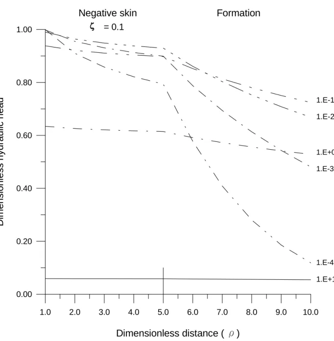
Figure 2 displays the curves of dimensionless hydraulic head versus dimensionless distance for rDs = 5, á = 10-5, and â ranging from 10-4 to 10 when (a) æ = 0.1, (b) æ = 1,
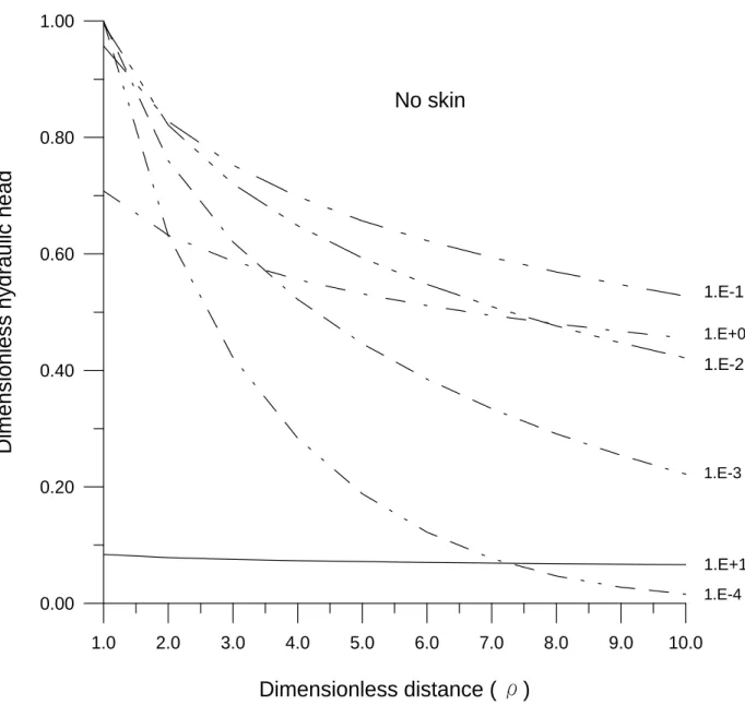
and (c) æ = 10. For the case without a skin zone, the dimensionless hydraulic head
gradually decreases when increasing radial distance and time as shown in Figure 2b. If a finite-thickness skin presents, both Figures 2a and 2c demonstrate that the relation of dimensionless hydraulic head versus dimensionless distance exhibits two curves with different slope joined at the interface (rDs = 5). A negative skin, which has a
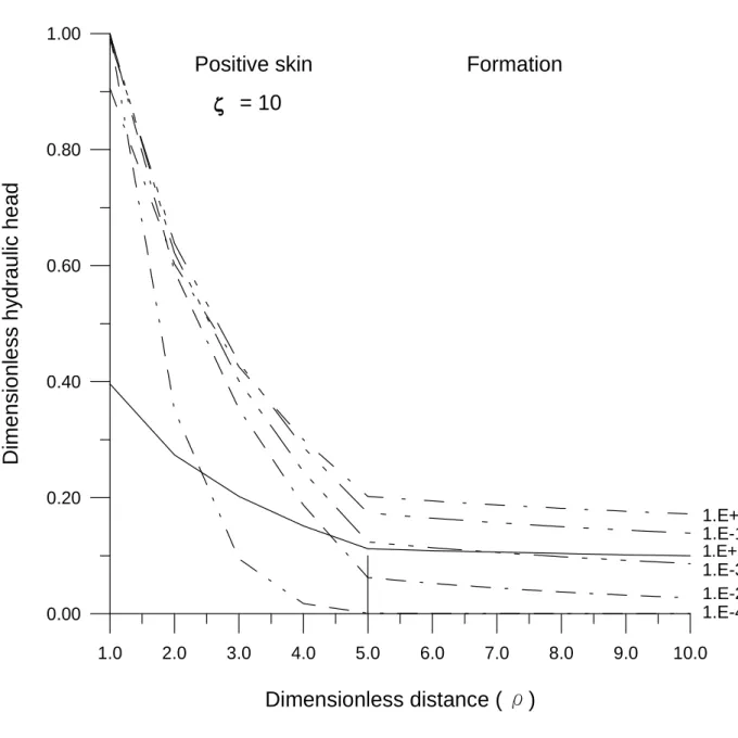
higher transmissivity than the formation, has a curve with relative mild slope in the skin zone and with steeper slope in the formation zone. In contrast, a positive skin has a very steep slope in the skin zone due to the lower transmissivity and a relative flat slope in the formation zone. The dimensionless hydraulic head always decreases with increasing dimensionless time (â); on the other hand, the dimensionless
hydraulic head in the formation zone increases for a period of time, and then decreases at large time (say, â > 1 or 10) as indicated in the figures. In addition, the
dimensionless hydraulic head of a negative skin more quickly stabilizes than that of a positive skin. Obviously, the dimensionless hydraulic head distributions are significantly effected by the properties of skin.
4.2 Effect of finite thickness skin
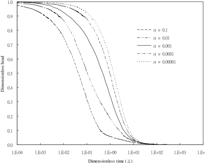
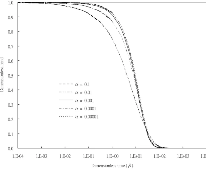
Figures 3a and 3b show a plot of dimensionless hydraulic head versus dimensionless time for rDc = 0.5, rD = 1, rDs = 10, ç = 1, and ζ = 0.1 or 10 while α
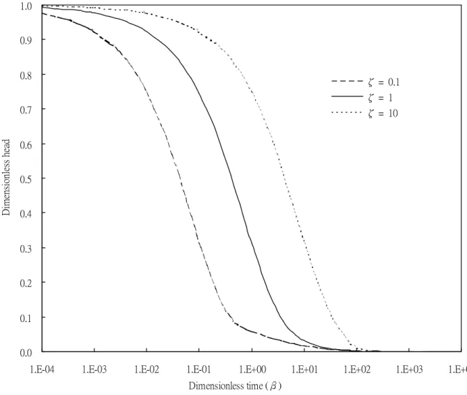
= 10-1 to 10-5. The formation has a negative skin while ζ = 0.1 and a positive skin when ζ =10. The dimensionless hydraulic head values obtained by the numerical Laplace inversion agree well with that of the closed-form solution. This indicates that the closed-form solution yields accurate results for the presence of a wellbore skin when estimated by the proposed numerical approach. Figures 4a and 4b show that the curve representing the dimensionless hydraulic head for the undisturbed (single-layer) formation is quite different from that with a positive or negative wellbore skin. If a positive wellbore skin exists, the dimensionless hydraulic head is smaller than that when a negative wellbore skin exists at the same dimensionless time. A smaller dimensionless hydraulic head reflects the result of lower hydraulic conductivity of the positive skin. Conversely, a larger dimensionless hydraulic head is considered to reflect the increase of formation conductivity and storage effects in the presence of a negative wellbore skin.
4.3 Effect of different skin thickness
To investigate the influence of skin thickness, Figures 5a and 5b show two sets of type curves for rDc = 0.5, rD = 1, α = 10-5, ç = 1 and ζ = 0.1 or 10 while rDs = 5,
10, 50, or 100. The results show that the skin thickness effects the dimensionless hydraulic head at early time, as β ranged from 10-1 to 10. However, the dimensionless hydraulic head diminishes to zero at a large dimensionless time. For a positive wellbore skin condition, the dimensionless hydraulic head decreases with increasing skin thickness. Conversely, the dimensionless hydraulic head increases with increasing skin thickness in the presence of a negative wellbore skin.
4.4 Effect of Contr ast of Tr ansmissivity
A plot of dimensionless well water level versus dimensionless time for rDs = 10
and á = 10-5 when æ = 0.1, 0.5, 1, 5, or 10 is displayed in Figure 6. In this figure, the
dimensionless well water level curves for the system with a negative skin are presented by æ = 0.1 and 0.5, without skin by æ = 1, and with a positive skin by æ = 5
and 10. The dimensionless well water level increases with α values under the same dimensionless time and is significantly affected by the positive skin than by the negative skin. Lower transmissivity of the positive skin produces lower flow rate toward the formation and results in higher dimensionless well water level. On the other hand, larger transmissivity of the negative skin yields larger flow rate across the wellbore and results in smaller dimensionless well water level. The dimensionless well water levels are larger for the system with a positive wellbore skin than those without wellbore skin at the same dimensionless time. From Figure 6, the differences of dimensionless well water level between the two-layer and uniform medium systems are negligible at small- and large-dimensionless times (i.e., β < 10-1, β > 103). On the other hand, the observed differences of dimensionless well water level are quite large at intermediate-dimensionless time.
5.
Conclusions
A closed-form solution for a two-layer confined ground-water system has been developed for slug test in a well with the presence of a wellborn skin. This solution was derived using Laplace transform and a contour integral method. In a single-layer aquifer system, comparisons of the dimensionless hydraulic head computed from the closed-form solution and the Laplace-domain solution with the dimensionless hydraulic head given by Cooper et al. (1967) agree to four decimal places. Under a two-layer condition, i.e., in the presence of a positive or negative wellbore skin, the results of the closed-form solution agree with those of the Laplace-domain solution to five decimal places. This provides a double check for the correctness of the closed-form solution.
The dimensionless hydraulic head decreases rapidly with increasing dimensionless time at early stage of the slug test and asymptotically approaches a constant value for a long test period. For small times the differences between the dimensionless hydraulic head in an aquifer with a positive or negative wellbore skin and an aquifer without a wellbore skin are large. In addition, the effect of a negative wellbore skin on the dimensionless hydraulic head is larger than that of a positive wellbore skin. Obviously, the magnitude of the dimensionless hydraulic head strongly depends on the hydraulic properties of both the formation and the wellbore skin.
Refer ences
Abramowitz, M., and I. A. Stegun, editors, Handbook of Mathematical Functions With Formulas, Graphs and Mathematical Tables, Dover, Publications, Inc., New
York, 1964.
Bredehoeft, J. D., H. H. Cooper, Jr., and I. S. Papadopulos, Inertial and storage effects in well-aquifer systems: An analog investigation, Water Resour. Res., 2(4),
697–707, 1966.
Butler, J. J. Jr., The design, performance, and analysis of slug tests. Boca Raton,
Lewis Publishers, 1997.
Butler, J. J. Jr., and J. M. Healey, Relationship between pumping-test and slug-test parameters: Scale effect or artifact?, Ground Water, 36(2), 305-313, 1998.
Carslaw, H. S., and J. C. Jaeger,Conduction of heat in solids, second ed., Clarendon
Press, Oxford, UK, 1959.
Cooper, Jr., H. H., J. D. Bredehoeft, and I. S. Papadopuls, Response of a finite–diameter well to an instantaneous charge of water,Water Resour. Res., 3(1),
263-269, 1967.
Crump, K. S., Numerical inversion of Laplace transforms using a Fourier series approximation, J. Assoc. Comput. Mach., 23(1), 89-96, 1976.
de Hoog, F. R., J. H. Knight, and A. N. Stokes, An improved method for numerical inversion of Laplace transforms,Society for Industrial and Applied Mathematics, J. Sci. Stat. Comput., 3(3), 357-366, 1982.
Faust, C. R., and J. W. Mercer, Evaluation of slug tests in wells containing a finite-thickness skin, Water Resour. Res., 20(4), 504-506, 1984.
Ferris, J. G., and D. B. Knowles, The slug test for estimating transmissibility, U. S. Geological Survey Ground Water Note, 26, 1-7, 1954.
Hildebrand, F. B.,Advanced calculus for applications, second ed., Prentice-Hall, Inc.,
Englewood Cliffs, NJ, 1976.
International Mathematics and Statistics Library, Inc., IMSL User's Manual, Vol. 2,
IMSL, Inc., Houston, TX, 1987.
Karasaki, K., J. C. S. Long, and P. A. Witherspoon, Analytical models of slug tests,
Water Resour. Res., 24(1), 115-126, 1988.
Karasaki, K., A systematized drillstem test, Water Resour. Res., 26(12), 2913-2919,
1990.
Kipp, Jr, K. L., Type curve analysis of inertial effects in the response of a well to a slug test,Water Resour. Res., 21(9), 1397-1408, 1985.
Water Resour. Res., 25(11), 2388-2396, 1989.
Moench, A. F., and P. A. Hsieh, Comment on “Evaluation of slug tests in wells containing a finite-thickness skin” by C. R. Faust and J. W. Mercer, Water Resour. Res., 21(9), 1459-1461, 1985.
Pandit, N. S., and R. F. Miner, Interpretation of slug test data, Ground Water, 24(6),
743-749, 1986.
Peng, H. Y., H. D. Yeh, and S. Y. Yang, Improved numerical evaluation of the radial groundwater flow equation, Advances in Water Resources, 2002. (In press)
Ramey, Jr., H. J., and R. G. Agarwal, Annulus unloading rates as influenced by wellbore storage and skin effect,Soc. Pet. Eng. J., 453-463, 1972.
Ramey, H. J., Jr., R. G. Agarwal, and I. Martin, Analysis of “Slug Test” or DST flow period data,J. Can. Pet. Technol., 37-47, 1975.
Sageev, A., Slug test analysis,Water Resour. Res., 22(8), 1323-1333, 1986.
Shanks, D., Non-linear transformations of divergent and slowly convergent sequences,
J. Math. Phys., 34, 1-42, 1955.
Spiegel, M. R., Laplace Transforms, Schaum Publishing Co., NY, 1965.
Watson, G. N., A Treatise on the Theory of Bessel Functions, second ed., Cambridge
University Press, UK, 1958.
Wynn, P., On a device for computing the em(Sn) transformation, Math. Tables Other Aids Comp., 10, 91-96, 1956.
Yang, Y. J., and T. M. Gates, Wellbore skin effect in slug-test data analysis for low-permeability geologic materials,Ground Water, 35(6), 931-937, 1997.
Yang, S. Y., and H. D. Yeh, A solution for flow rates across the wellbore in a two-layer confined aquifer, J. Hydraul. Eng. ASCE, 128(2), 175-183, 2002.
Table 1. Dimensionless hydraulic head versus dimensionless time (â) estimated by the
closed-form solution, the numerical inversion from the Laplace-domain solution, and the one given in Cooper et al. (1967) for rDc = 0.5, rD = 1,rDs = 10, and ζ = ç = 1
when α = 10-1 or 10-5. á = 10-1 á = 10-5 â NS CS Cooper NS CS Cooper 0.01 0.92385 0.92384 0.9238 0.99417 0.99417 0.9942 0.02 0.89036 0.89036 0.98942 0.98942 0.03 0.86425 0.86425 0.98496 0.98496 0.04 0.84208 0.84208 0.98069 0.98069 0.05 0.82249 0.82249 0.97654 0.97654 0.06 0.80477 0.80477 0.97251 0.9725 0.07 0.78850 0.78850 0.96855 0.96855 0.08 0.77339 0.77339 0.96467 0.96467 0.09 0.75926 0.75926 0.96086 0.96086 0.1 0.74595 0.74595 0.7460 0.95710 0.95710 0.9572 0.2 0.64182 0.64182 0.92183 0.92183 0.3 0.56751 0.56751 0.88953 0.88953 0.4 0.50954 0.50954 0.85936 0.85936 0.5 0.46229 0.46229 0.83091 0.83091 0.6 0.42273 0.42273 0.80394 0.80394 0.7 0.38897 0.38897 0.77827 0.77827 0.8 0.35976 0.35976 0.75378 0.75378 0.9 0.33421 0.33421 0.73036 0.73036 1 0.31166 0.31166 0.3117 0.70794 0.70794 0.7080 2 0.17856 0.17856 0.52628 0.52628 3 0.11957 0.11957 0.39920 0.39920 4 0.08761 0.08761 0.30754 0.30754 5 0.06814 0.06814 0.24017 0.24017 6 0.05527 0.05527 0.18995 0.18995 7 0.04625 0.04625 0.04625 0.15208 0.15208 0.1521 8 0.03963 0.03963 0.12322 0.12322 9 0.03459 0.03459 0.10102 0.10102 10 0.03065 0.03065 0.03065 0.08378 0.08378 0.08378 20 0.01408 0.01408 0.02256 0.02256 30 0.00907 0.00907 0.009070 0.01169 0.01169 0.01169 40 0.00668 0.00668 0.00790 0.00790 50 0.00528 0.00528 0.00599 0.00599 60 0.00437 0.00437 0.00483 0.00483 70 0.00372 0.00372 0.003722 0.00405 0.00405 0.004046 80 0.00324 0.00324 0.00348 0.00348 90 0.00287 0.00287 0.00306 0.00306 100 0.00258 0.00258 0.002577 0.00272 0.00272 0.002725 200 0.00127 0.00127 0.00131 0.00131 300 0.00084 0.00084 0.00086 0.00086 400 0.00063 0.00063 0.00064 0.00064 500 0.00050 0.00050 0.00051 0.00051 600 0.00042 0.00042 0.00042 0.00042 700 0.00036 0.00036 0.00036 0.00036 800 0.00031 0.00031 0.00032 0.00032 900 0.00028 0.00028 0.00028 0.00028 1000 0.00025 0.00025 0.00025 0.00025
T
2Confining layer
Confining layer
r
wFormation zone
Wellbore
Skin zone
r
cT
1Well screen
r
SH
iH
01.0 2.0 3.0 4.0 5.0 6.0 7.0 8.0 9.0 10.0
Dimensionless distance ( ρ)
0.00 0.20 0.40 0.60 0.80 1.00D
im
e
n
s
io
n
le
s
s
h
y
d
ra
u
lic
h
e
a
d
1.E-4 1.E-3 1.E+1 1.E+0 1.E-1 1.E-2 = 0.1Negative skin
Formation
Figure 2a. Plots of dimensionless hydraulic head versus dimensionless time forrDs =
1.0 2.0 3.0 4.0 5.0 6.0 7.0 8.0 9.0 10.0 Dimensionless distance ( ρ) 0.00 0.20 0.40 0.60 0.80 1.00 D im e n s io n le s s h y d ra u lic h e a d 1.E-4 1.E-3 1.E+1 1.E+0 1.E-1 1.E-2 No skin
Figure 2b. Plots of dimensionless hydraulic head versus dimensionless time for rDs
1.0 2.0 3.0 4.0 5.0 6.0 7.0 8.0 9.0 10.0 Dimensionless distance ( ρ) 0.00 0.20 0.40 0.60 0.80 1.00 D im e n s io n le s s h y d ra u lic h e a d 1.E-4 1.E-3 1.E+1 1.E+0 1.E-1 1.E-2 = 10 Formation Positive skin
Figure 2c. Plots of dimensionless hydraulic head versus dimensionless time for rDs =
0.0 0.1 0.2 0.3 0.4 0.5 0.6 0.7 0.8 0.9 1.0
1.E-04 1.E-03 1.E-02 1.E-01 1.E+00 1.E+01 1.E+02 1.E+03 1.E+04 Dimensionless time (β) Dimensionless head α = 0.1 α = 0.01 α = 0.001 α = 0.0001 α = 0.00001
Figure 3a. A plot of dimensionless hydraulic head versus dimensionless time for rDc
0.0 0.1 0.2 0.3 0.4 0.5 0.6 0.7 0.8 0.9 1.0
1.E-04 1.E-03 1.E-02 1.E-01 1.E+00 1.E+01 1.E+02 1.E+03 1.E+04 Dimensionless time (β) Dimensionless head α = 0.1 α = 0.01 α = 0.001 α = 0.0001 α = 0.00001
Figure 3b. A plot of dimensionless hydraulic head versus dimensionless time for rDc
0.0 0.1 0.2 0.3 0.4 0.5 0.6 0.7 0.8 0.9 1.0
1.E-04 1.E-03 1.E-02 1.E-01 1.E+00 1.E+01 1.E+02 1.E+03 1.E+04 Dimensionless time (β)
Dimensionless head
ζ = 0.1 ζ = 1 ζ = 10
Figure 4a. A plot of dimensionless hydraulic head versus dimensionless time for rDc
0.0 0.1 0.2 0.3 0.4 0.5 0.6 0.7 0.8 0.9 1.0
1.E-04 1.E-03 1.E-02 1.E-01 1.E+00 1.E+01 1.E+02 1.E+03 Dimensionless time (β)
Dimensionless head
ζ = 0.1 ζ = 1 ζ = 10
Figure 4b. A plot of dimensionless hydraulic head versus dimensionless time for rDc
0.0 0.1 0.2 0.3 0.4 0.5 0.6 0.7 0.8 0.9 1.0
1.E-04 1.E-03 1.E-02 1.E-01 1.E+00 1.E+01 1.E+02 1.E+03 Dimensionless time (β) Dimensionless head rs/rw = 5 rs/rw = 10 rs/rw = 50 rs/rw = 100
Figure 5a. A plot of dimensionless hydraulic head versus dimensionless time for rDc
0.0 0.1 0.2 0.3 0.4 0.5 0.6 0.7 0.8 0.9 1.0
1.E-04 1.E-03 1.E-02 1.E-01 1.E+00 1.E+01 1.E+02 1.E+03 1.E+04 Dimensionless time (β) Dimensionless head rs/rw = 5 rs/rw = 10 rs/rw = 50 rs/rw = 100
Figure 5b. A plot of dimensionless hydraulic head versus dimensionless time for rDc
1.0E-2 1.0E-1 1.0E+0 1.0E+1 1.0E+2 1.0E+3 1.0E+4 Dimensionless time (β ) 0.00 0.20 0.40 0.60 0.80 1.00 D im e n s io n le s s w e ll w a te r le v e l Symbol
ζ
0.1 0.5 1 5 10Figure 6. A plot of dimensionless well water level versus dimensionless time forrDs
計畫成果自評
本研究第一年計畫,係針對完全貫穿受壓含水層之徑向雙層水流方程式, 利用 Laplace 逆轉換和 Bromwich contour 積分,推導得一個新的時間域閉合解。 經 Laplace 逆轉所求得時間域的閉合解,如(9)和(10)式所示,具有積分式且積分 範圍從零到無限大,積分函數包含 Bessel 函數相乘積,在數值計算上,首先以 bisection 方法尋找積分函數的根,以 Gaussian quadrature 計算相鄰兩根間的面 積;接著,視相鄰兩根間的面積值為無限級數中的一項,將積分式轉換為一個累 加的無窮級數;最後,利用 Shanks 方法(Shanks, 1955)以加速 Bessel 函數和級 數的收斂。閉合解數值計算結果,與用 IMSL 的修正 Crump 方法對 Laplace 域解 做數值逆轉所得數值比較,吻合的精度,達小數後五位。利用這個閉合解,可繪 製類似 Theis 方法的標準曲線,以利工程應用;此外,針對井膚層的厚度及特性, 可量化分析微水試驗時水層參數對水力水頭在時空上分佈的影響。
目前我們已完成上述數值計算分析,並完成期刊論文撰寫初稿,擬於 6 月 初投稿到國外期刊。
第二年計畫,擬考慮水井部份貫穿的情況,利用 Laplace 轉換和 finite cosine 轉換,以推導徑向雙層水流方程式的 Laplace 域水層水頭半解析解,再利用 finite cosine 逆轉換,可求得水層水力水頭和井緣流量的 Laplace 域解,此解可用來探 討井膚層和部份貫穿井兩者的效應,對微水試驗數據分析的影響。
Appendix A: Der ivation of (14)
The inverse Laplace transforms of (10) in the time domain can be obtained using the Laplace inversion integral (Hildebrand, 1976) as
dp h e i h i i pt 1 1 2 1
∫
−+∞∞ = ξξ π (A1)where p = complex variable; i = imaginary unit; and î = large, real, and positive
constant, so that all the poles lie to the left of line (î- i∞,î+ i∞).
A single branch point with no singularity (pole) at p = 0 exists in the integrand of
(10). Thus, this integration may require using the Bromwich integral for the Laplace inversion. The closed contour of integrand is shown in Figure A with a cut of p
plane along a negative real axis, where ä is taken sufficiently small to exclude all poles from the circle about the origin. The closed contour consists of the part AB of
the Bromwich line from minus infinity to infinity, semicircles BCD and GHA of
radius R, lines DE and FG parallel to the real axis, and a circle EF of radius ä about a
origin. The integration along the small circle EF around a origin as ä approaches
zero is carried out using the Cauchy integral and the value of the integration is equal to zero. The integrals taken along BCD and GHA tend to zero as R approaches
infinity. Consequently, (10) can be superseded by the sum of integrals along DE and FG. In other words, the integral can be written as
+ =
∫
∫
∞ → → i e hdp e hdp h FG pt DE pt R 1 1 0 1 2 1 lim π δ (A2)For the first term on the right-hand-side (RHS) of (A2) along DE, we introduce
the new variable 2 1 1 /S T e u
p= −πi and use the formulas (Carslaw and Jaeger, 1959, p.490)
( )
( )
[
J z iY z]
ie ze Kv i =± vi − v ± v ± π π π 2 1 2 1 2 1 m (A3) and( )
z J e ze Iv πi 2vπi v 1 2 1 ± ± = (A4)where v = 0, 1, 2, . . .. The first term on the RHS of (A2) then leads to
( )
( )
[
]
( )
( )
[
]
du u iB u B u iA u A e i H r h t u S T w DE 2 1 1 2 0 0 1 2 1 1 + − − =∫
∞ − π η (A5) Likewise, introducing 2 1 1 /S T e up= πi , the integral along FG gives minus the
( )
( )
[
]
( )
( )
[
]
du u iB u B u iA u A e i H r h t u S T w FG 2 1 2 1 0 0 1 2 1 1 − + =∫
∞ − π η (A6)Figure A. A plot of the closed contour integration of h for the Bromwich integral (Hildebrand, 1976).