圓形可變樣板應用於眼睛張開程度偵測

國 立 交 通 大 學

電 機 與 控 制 工 程 研 究 所

碩 士 論 文

圓形可變樣板應用於眼睛張開程度偵測

Circular Deformable Template Application in Eye

Openness Detection

研 究 生 ： 徐 亦 澂

指 導 教 授： 張 志 永

圓形可變樣板應用於眼睛張開程度偵測

Circular Deformable Template Application in Eye

Openness Detection

學 生 : 徐亦澂 Student : Yi-Cheng Hsu

指導教授 : 張志永 Advisor : Jyh-Yeong Chang

國立交通大學

電機與控制工程學系

碩士論文

A Thesis

Submitted to Department of Electrical and Control Engineering

College of Electrical Engineering and Computer Science

National Chiao Tung University

in Partial Fulfillment of the Requirements

for the Degree of Master in

Electrical and Control Engineering

September 2007

Hsinchu, Taiwan, Republic of China

圓形可變樣板應用於眼睛張開程度偵測

學生: 徐亦澂

指導教授: 張志永博士

國立交通大學電機與控制工程研究所

摘要

在許多交通事故中，疲勞駕駛導致意外發生的事件層出不窮。於駕駛環境 下，使用不妨礙駕駛人的視訊設備，觀測駕駛者眼睛的狀況，以達成瞌睡偵測是 最直接有效的。亦即，經由偵測人眼開闔狀態來判斷是否出現瞌睡情形是相當準 確可靠之方法。在此篇論文中，我們以彩色 CCD 攝影機做為影像輸入來源，經過 膚色判定來區分出人臉區域，再以主成份分析法擷取出眼部區域，再利用圓形可 變樣版搜尋此區域，找出瞳孔的位置並加以分析之，以此判定眼睛此時的張開狀 態。經實驗證明，我們提出的方法於判定眼睛狀態的準確度相當高，將有助於提 高昏睡偵測系統的成功率。

Circular Deformable Template Application in Eye

Openness Detection

STUDENT: YI-CHENG HSU ADVISOR: JYH-YEONG CHANG

Institute of Electrical and Control Engineering National Chiao-Tung University

Abstract

Sleepiness and driving is a dangerous combination, drowsy driving can be just as fatal. Accordingly, it is necessary to develop a drowsy driver awareness system. To

avoid interrupting the driver, it is necessary to build a system under non-invasive and non-contact condition. Image process system suits to achieve such a request. Hence, it is recommended to judge the drowsiness state by observing eye status of operators via eye video. In this thesis, we use a CCD camera as the image sources and use skin color map to segment skin region. Then we use PCA algorithm to find the eye region for circular template searching. The circular template will locate the iris region and finally we can analyze this region to classify the eye openness state. By numerical simulation, we have obtained a high accuracy on eye openness detection and it would be helpful for the drowsy detection system.

ACKNOWLEDGEMENT

I would like to express my sincere appreciation to my advisor, Dr. Jyh-Yeong Chang. Without his patient guidance and inspiration during the two years, it is impossible for me to overcome the obstacles and complete the thesis. In addition, I am thankful to all my lab members for their discussion and suggestion.

Finally, I would like to express my deepest gratitude to my parents. Without their fully support and encouragement, I could not go through these two years.

Contents

摘要 ………….……….………i ABSTRACT ………ii ACKNOWLEDGEMENT ………iv CONTENTS ……….……..v LIST of FIGURES……….………vii LIST of TABLES…………..……….………vii CHAPTER 1 INTRODUCTION ………...1 1.1 Motivation ...……….……..2 1.2 Face Segmentation………...………….….………....2 1.3 Eye Detection……….………..……….4 1.4 I r i s E x t r a c t i o n … … … . . . … … … … . . … … … 4

1.5 Eye State Determination………5

1.6 Thesis Outline………5

CHAPTER 2 FACE SEGMENTATION……….…………..………...6

2.1 YCbCr Color Space………...………..………6

2.2 Face Segmentation Algorithm……….………7

CHAPTER 3 EYE DETECTION AND IRIS EXCTRATION…….14

3.1 PCA Review……….………..……….………14

3.2 Computation of Eigeneyes ….………...………15 3.3 R e p r e s e n t i n g E y e s o n t o T h i s B a s i s . . . … … … 1 7

3.4 Eye Region Recognition Using Eigeneyes………...17

3.5 Using Deformable Template for Iris Extraction………18

3.5.1 Intensity Field and Edge Field…………..………..19

3.5.2 A n i s o t r o p i c D i f f u s i o n … … … . … … … . . 2 0 3.5.3 Circular Deformable Template……….…….24

CHAPTER 4 EYE STATE DETERMINATION……….….28

4.1 Analyzing the Iris Region..………...………...28

4.2 Determining Eye State……….………..30

4.3 Drowsy State Detection….……….32

CHAPTER 5 EXPERIMENT RESULT……….. 34

5 . 1 E x p e r i m e n t S e t t i n g . . … … … . . … … … . . . 3 4 5 . 2 E x p e r i m e n t R e s u l t . . … … … . . … … … . … … … . . . 3 5 CHAPTER 6 CONCLUSIONS AND FUTURE WORK……..……….. 42

List of Figures

Fig. 2.1. Flowchart of the face-segmentation algorithm……….…………. 7

Fig. 2.2. Input image………...………9

Fig. 2.3. Output image after segmented by skin-color map in stage A…………9

Fig. 2.4. The procedure of doing density map D x y ………10 ( , )

Fig. 2.5. Density map after classified to three classes………..…………..11

Fig. 2.6. Output image produced by erode and dilate……..……….12

Fig. 2.7. Output image produced after stage C………..…………13

Fig. 2.8. Image produced by stage D………..……….………13

Fig. 3.1 Represent input eye region matrix to a vector……..……….……15

Fig. 3.2 An eye region image of edge field and intensity field…………..19

Fig. 3.3. The stepping function g(.)………...21

Fig. 3.4. Local neighborhood of pixels at a boundary………..22

Fig. 3.5. A diagram of anisotropic diffusion algorithm………..………….22

Fig. 3.6. An eye image after anisotropic diffusion……….………23

Fig. 3.7. An example of anisotropic diffusion algorithm……….23

Fig. 3.8. Eliminating the horizontal edges………24

Fig. 3.9. The diagram of circular template model………...25

Fig. 3.10. Examples of iris extraction………..………...27

Fig. 4.1. Physiological motion of human eye………..29

Fig. 4.2. Observable ratio of the iris appearance………..29

Fig. 4.3. Different level of eye closure and its hue component………31

Fig. 4.4. Flowchart of entire drowsy detection system…….………….………….33

Fig. 5.1. Different observable ratio of the iris of sample 1………35

Fig. 5.3. Different observable ratio of the iris of sample 3………37 Fig. 5.4. Different observable ratio of the iris of sample 4………38 Fig. 5.5. Observable ratio of the iris (L1) and hue ratio of the eye region (L2).…..39

List of Tables

Table I. Major face detection approaches ……….. 3 Table II. Accuracy of three eye states detection ………..………41

Chapter 1 Introduction

Sleepiness causes vehicle crashes because it impairs performance and can ultimately lead to the inability to resist falling asleep at the wheel. Critical aspects of driving impairment associated with sleepiness are reaction time, vigilance, attention, and information processing. A driver’s drowsiness is conceived as one of the major cause of traffic accidents. An intelligent warning system based on an automatic detection of the human physiological phenomena related to the drowsy state, would help to prevent car collision. In order to achieve this purpose, a driver’s drowsy state must be detected instantaneously.

Eyes are the most important features of human face. There are many applications of the robust eye states extraction. For example, the eye states provide important feature for recognizing facial expression and human-computer interface systems. When man is laughing, his eyes are nearly closed. And when he is surprised, his eyes are opened wide. The eye states can be got from the eye features such as the inner corner of eye, the outer corner of eye, iris, eyelid, eye position and so on. There are many methods to detect eye features. Yuille, Hallinan and Cohen [1] used deformable templates to locate eye features. Deng and Lai [2] used improved deformable templates to locate eye features.

Recently, a lot of research is actively conducted to build human-computer interface systems of high performance. An automatic and robust technique to extract the eye states from input images is very important in this field. In this thesis, we attempt to adopt some techniques to deal with this condition as well.

1.1 Motivation

Driver fatigue is a significant factor in a large number of vehicle accidents. Recent statistics estimate that annually 1,200 deaths and 76,000 injuries can be attributed to fatigue related crashes [3]. By monitoring the eyes, it is believed that the symptoms of driver fatigue can be detected early enough to avoid a car accident. Detection of fatigue involves a sequence of images of a face, and the observation of eye position and blink patterns.

The analysis of face images is a popular research area with applications such as face recognition, virtual tools, and human identification security systems. This thesis is focused on the localization of the eyes, which involves looking at the entire image of the face, and determining the position of the eyes by a self developed image processing algorithm. Once the position of the eyes is located, the system is designed to determine whether the eyes are opened or closed, and then detect his fatigue state if necessary.

1.2 Face Segmentation

When we get an input image from the image sequence of frontal view of faces, it always contents the human face and background. If we search for the eye in the whole image, the background would deteriorate the result sharply and complicate computation. In order to reduce the region for eye search and find the eye position more accurately, we need to do face segmentation initially. There are many methods or algorithms have been proposed for face detection in recent years. According to Hjelmas and Low [4], the major approaches are listed in Table I. These approaches utilize techniques such as principal component analysis, neural networks, machine

learning, information theory, geometrical modeling, deformable template matching, Hough transform, motion extraction, and color analysis. Among these methods above, color analysis is a straightforward method and provides useful cue for face detection.

TABLE I

Major Face Detection Approaches

Authors Year Approach Feature Used Head Pose Test Databases Féraud et al. [5] 2001 Neural Networks Motion; Color;

Texture

Frontal and profile

Sussex; CMU; Web images

Maio et al. [6] 2000 Facial Templates; Hough Transform Texture; Directional images Frontal to near frontal Static images

Garcia et al. [7] 1999 Statistical wavelet analysis Color; wavelet coefficients

Frontal to profile

MPEG videos

Wu et al. [8] 1999 Fuzzy color models; Template matching

Color Frontal Still color images

Rowley et al.[9] 1998 Neural Networks Texture Frontal CMU;FERET; Web images

Sung et al. [10] 1998 Learning Texture Frontal Mug shots; CCD pictures;

Newspaper scans

Yang et al. [11] 1998 Multiscale segmentation; color model

Skin Color; intensity

Frontal Color pictures

Colmenarez et

al. [12]

1997 Learning Markov

processes

Frontal FERET

Yow et al. [13] 1997 Feature; Belief networks Geometrical facial feature

Frontal to profile

CMU

Lew et al. [14] 1996 Markov Random Field; DFFS.

Most informative pixel

Frontal MIT; CMU;

1.3 Eye Detection

After we separate the background and face from a mug image, there is properly an output image with only skin color region. It is difficult to search for the iris in the skin color region because the search region is still too large. Obviously, before any of the components of the eye can be extracted and fitted, the eye have first to be located in the face. Donato et al. [15] compared several techniques for recognizing upper face images and lower face images. These techniques include optical flow, principal component analysis, independent component analysis, local feature analysis, and Gabor wavelet representation. The best performance was achieved by principle component analysis (PCA). We therefore start with the PCA estimated eye locations so we can then set up a good search region for the iris.

1.4 Iris Extraction

In facial expression analysis, the motion of eyes is important to express the expressions. In driver behavior analysis application, the car should send visual or auditory signals to get the driver’s attention if the driver is found not attentive. In these applications, we need to know a detailed description of the eye besides the location of the eye. That is, we need to obtain the parameters of an eye model (e.g., the location and radius of the iris). There are many models proposed to describe the eye feature, such as chain codes, fitting line segments, autoregressive models, Fourier descriptors, active contour model and deformable template by Yuille et al. [1]. Among these models, the deformable template is an efficient model used for describing and tracking the contour of the eye. In this thesis, we use deformable template to extract iris region and its size will use to be define the state of eye openness.

1.5 Eye State Determination

Driver's eye state is a key factor for identifying the driver's visual attention. If someone comes to a fatigue situation, the duration time of his eye blinking will increase and the proportion of the closed state will longer to normal state. Accordingly, after we extracted the iris, then we can identify the eye state. To this goal, we want to decide the eye state by observing the iris image in RGB color map. In this thesis, we define three eye state: open, barely open, and closed. The detailed definition will be elaborated in the following chapter. So when an input image is classified to one state of them, we subsequently can calculate the subject’s PERCLOSE value. Namely, useful for driver’s sleepiness detection if it is in excess of the threshold of PERCLOSE, a warning signal will be triggered.

1.6 Thesis Outline

The contents of this thesis are organized as follows. In Chapter 2, the face segmentation algorithm will firstly be described, and the eye position detection and the iris extraction follow in Chapter 3. Then the iris extraction will be extended to analyze for eye state detection and definition of three eye states is proposed in Chapter 4. Then we do some simulations and show our experimental results of the methods in Chapter 5. In chapter 6, we give some conclusions and discuss future work to be investigated further.

Chapter 2 Face Segmentation

2.1 YCbCr Color Space

The first step in the face detection algorithm is using skin segmentation to reject as much “non-face” of the image as possible, since the main part of the images consists of background color pixels. There are two ways of segmenting the image based on skin color: converting the RGB color space to YCbCr color space or to HSV

color space. YCbCr space segments the image in pixels into a luminosity component Y

together with Cb and Cr and color components, whereas an HSV space defines the

image pixels by the three components of hue Y, saturation S,and intensity value V. The advantage of converting the image to the YCbCr color space is that the effect of

luminosity can be decoupled with coloring components during our image processing. In the RGB domain, each component red, green and blue of the picture element has a different strength value. However, in the YCbCr domain, the pixel’s intensity,

brightness, is given by the Y -component, since the Cb (blue) and Cr (red) components

are independent from the luminosity. The following conversion matrix are used to convert the RGB image into Y, Cb and Cr components [16]:

0.257 0.504 0.098 16 0.148 0.291 0.439 128 0.439 0.368 0.071 128 Y R Cb G Cr B ⎡ ⎤ ⎡ ⎤ ⎡ ⎤ ⎡ ⎤ ⎢ ⎥ ⎢_{= − −} ⎥ ⎢ ⎥ ⎢₊ ⎥ ⎢ ⎥ ⎢ ⎥ ⎢ ⎥ ⎢ ⎥ ⎢ ⎥ ⎢ − − ⎥ ⎢ ⎥ ⎢ ⎥ ⎣ ⎦ ⎣ ⎦ ⎣ ⎦ ⎣ ⎦ (2.1)

2.2 Face Segmentation Algorithm

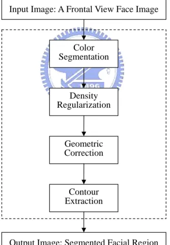
The algorithm in [17] is an unsupervised segmentation algorithm, and hence no manual adjustment of any design parameter is needed in order to suit any particular input image. The only principal assumption is that the person’s face must be present in the given image, since we are locating the face and not detecting whether there is a face. The revised algorithm we used is composed of four stages, as depicted in Fig. 2.1.

Fig. 2.1. Flowchart of the face-segmentation algorithm. Input Image: A Frontal View Face Image

Output Image: Segmented Facial Region Color Segmentation Density Regularization Geometric Correction Contour Extraction

A. Color Segmentation

The first stage of the algorithm is to classify the pixels of the input image into skin region and non-skin region. To do this, we obtain a skin-color reference map in YCbCr color space. It has been proved that a skin-color region can be identified by the

presence of a certain set of chrominance values (i.e., Cb and Cr) narrowly and

consistently distributed in the YCbCr color space. We utilize RCb and RCr to represent

the respective ranges of Cb and Cr values that correspond to skin color, which

subsequently define our skin-color reference map. The ranges to be most suitable for all the input images are

[

133, 173

]

r C R = and

[

77, 127

]

b C R = .

In order to reduce the computation time, we downsample, both row and column, the input image to half resolution and recover it in the last stage. Therefore, for an image of M×Npixels and we downsample it to M / 2×N/ 2. With the skin-color reference map, we got the color segmentation result OA as

( )

, 1, if ,

( )

( )

, 0, otherwise r b r C b C A C x y R C x y R O x y = ⎨⎧⎪ ⎡⎣ ∈ ⎤⎦ ⎣⎡ ∈ ⎤⎦ ⎪⎩ ∩ (2.2)

where x= 0, … , M/ 2 1− and y = 0, … , N/ 2 1− and M, N are height and width

of the input image respectively. An example of output image to illustrate the classification of the input image Fig. 2.2 is shown in Fig. 2.3.

Fig. 2.2. Input image.

Fig. 2.3. Output image after segmented by skin-color map in stage A.

B. Density Regularization

The bitmap produced by the preceding stage A to reserve the facial region is corrupted by noise. The noise may be small holes on the facial region due to undetected facial features such as eyes, mouth, and even glasses. It may also appear as

simple morphological operations such as dilation to fill in the small holes in the facial region and erosion to remove the small object in the background scene. To distinguish facial region form non-facial region, we first need to identify regions of the bitmap that have higher probability of being the facial region. For this task, a density mapD x y is calculated as follows. ( , )

( )

3 3

(

)

0 0 , _A 4 , 4y i j D x y O x i j = = =

∑∑

+ + (2.3) It first partitions the output bitmap of stage A OA(x, y) into non-overlapping

groups of 4×4 pixels, then counts the number of skin-color pixels within each group and assigns this value to the corresponding point of the density map.

Fig. 2.4. The procedure of doing density map D x y . ( , )

According to the density value, we classify each pixel into one of three clusters: zero (D = 0), intermediate (0 < D < 16), and full (D = 16). Fig. 2.5 shows the density map of the output bitmap of stage A shown in Fig. 2.3 with three density classifications. The point of zero density is shown in white, intermediate density in

green, and full density in black. A group of points with white color will likely represent a non-facial region, while a group of black points will signify a cluster of skin-color pixels and a high probability of belonging to a facial region. Points with intermediate density values shown in green will probably indicate the noise.

Fig. 2.5. Density map after classified to three classes.

After the density map is derived, we then begin the process that termed as density regularization. This includes three steps as below.

1) Discard all points at the edge of the density map, i.e., set D(0, y) = D(M/4–1, y) =

D(x, 0) = D(x, N/4–1) for all x = 0, 1, …, M/4–1 and y = 0, 1, …, N/4–1.

2) Erode any full-density point (i.e., set to zero) if it is surrounded by less than five other full-density points within its local 3×3 neighborhood.

3) Dilate any point with either zero or intermediate density (i.e., set to 16) if there are more than two full-density points within its local 3×3 neighborhood.

Processed by density regularization, the density map is converted to the output bitmap of stage B as

( )

1, if ,

( )

16 , 0, otherwise B D x y O x y = ⎨⎧ = ⎩ (2.4)

for all x = 0, 1, …, M/4–1 and y = 0, 1, …, N/4–1. The eroded and dilated result of the bitmap in Fig. 2.5 processed after stage B is shown in Fig. 2.6.

Fig. 2.6. Output image produced by erode and dilate.

C. Geometric Correction

After stage B, there may be still some fragmented areas in the output bitmap. In order to eliminate or mend these areas, we performed a horizontal and vertical scanning process to identify the presence of any odd structure in the preceding bitmap obtained from stage B, OB(x, y), and subsequently removed it. Firstly, we use a

technique similar to that introduced in stage B to further remove any more noise. A pixel in OB(x,y) with a value of one will remain as a detected facial pixel if there are

more than three other pixels with the same value in its local 3×3 neighborhood. Simultaneously, a pixel in OB(x,y) with a value of zero will be reconverted to a value

of one (i.e., as a potential pixel of the facial region) if it is surrounded by more than five pixels with a value of one in its local 3×3 neighborhood.

A bitmap of well-detected facial region should look continuous, and therefore any short run of pixels with the value different from the detected facial region should unlikely belong to this region. As a result, next to the process above, we then begin the horizontal scanning process on the filtered bitmap. We search for any short continuous run of pixels which are assigned with the value of one. Any group of less

than four horizontally connected pixels with the value of one will be eliminated and assigned to zero. A similar process is then performed in the vertical direction. After all processes in this stage, the output bitmap should contain the facial region with minimal or even no noise, as shown in Fig. 2.7.

Fig. 2.7. Output image produced after stage C.

D. Contour Extraction

In this stage, we convert the output bitmap of stage C back to the original dimension of the extracted face region from stage A. We utilize the edge information that is already made available by the color segmentation in stage A. All the boundary points in the previous bitmap will be mapped into the corresponding group of 4×4 pixels with the value of each pixel as defined in the output bitmap of stage A. The output image of this final stage is shown in Fig. 2.8.

Fig. 2.8. Image produced by stage D.

Chapter 3 Eye Detection and Iris Extraction

3.1 PCA Review

Most approaches in computer recognition of faces and expressions have been focused on detecting individual features such as eyes, head outline, mouth, or defining a face model by position, size, and relationships among these features. Features extraction plays an essential role in the pre-processing stage. Principal component analysis (PCA) has been commonly used to face recognition problems [18]. Typical PCA algorithm is one of the main streams of research on face feature processing [19]. PCA has advantage over other face recognition schemes in its speed and simplicity. We utilized PCA in the pre-processing stage to extract features from input face image which has been segmented by skin color mentioned in chapter 2.

The basis of the input image space is composed of all single pixel vectors. However, the input image space is not an optimal space for face representation and categorization. The aim of applying PCA is to build an eye space which better describes the eye regions. The basis vectors of this eye space are called the principal components. These components will be uncorrelated and will maximize the variance accounted in the original basis. It can also reduce the dimension of the feature space. The computation complexity is thus reduced.

3.2 Computation of Eigeneyes

Step 1: obtain eye region imagesI I1, 2, ,IM(training eyes)

important note: the eye region images must be the same size.

Step 2: represent every input image as a vector Γ i

Fig.3.1 Represent input eye region matrix to a vector

Step 3: compute the average eye vector Ψ :

1

1

M i i

M

₌

Ψ =

∑

Γ

_(3.1)

Step 4: subtract the average eye vector Ψ:

i _i

Step 5: compute the covariance matrix C: 2 2 1 1 ( matrix) M T T n n n C AA N N M ₌ =

∑

Φ Φ = × (3.3)

Step 6: compute the eigenvectors ui of AA T

The matrix AA is very large (T N2×N2), so it is not practical to compute the eigenvectors ui of AA . T

Step 6.1: consider the matrix A A MT ( ×M matrix) Step 6.2: compute the eigenvector vi of A A T

(3.4) Observe the relationship between ui and v : i

or

where

T T i i i i i i i i i i i i i i

A Av

v

AA Av

Av

CAv

Av

Cu

u

u

Av

μ

μ

μ

μ

=

⇒

=

⇒

=

=

=

Thus, AAT and A AT have the same eigenvalues and their eigenvectors are related as follows: ui =Avi

Note 1: AA can have at most T N2 eigenvalues and eigenvectors. Note 2: A A can have at most M eigenvalues and eigenvectors. T

Note 3: The M eigenvalues of A A correspond to the M largest eigenvalues of T

2 1 2 where A= Φ Φ[ ΦM] (N ×M matrix ) T i i i

A

A v

=

μ

v

T

AA and in the same way as eigenvectors.

Step 6.3: normalize uisuch that ui =1, compute M best eigenvectors of

T

AA for ui =Avi.

Step 7: keep M eigenvectors which are corresponding to the M largest eigenvalues.

3.3 Representing Eyes onto PCA Basis

Each eye region image (minus the mean) Φ in the training set can be represent i as a linear combination of the M eigenvectors:

1 ˆ M _{, ( =} T ₎ i j j j j i j mean w u w u = Φ − =

∑

Φ (3.5)

Each normalized training eye region image Φ is represent in this basis by a i vector: 1 2 , 1, 2, , i i i i M w w i M w ⎡ ⎤ ⎢ ⎥ ⎢ ⎥ Ω = _{⎢ ⎥} = ⎢ ⎥ ⎢ ⎥ ⎣ ⎦ … (3.6)

3.4 Eye Region Recognition Using Eigeneyes

Input an unknown eye region image Γ with the same size as training image and follow these steps:

Step 1: normalize Γ : Φ = Γ − Ψ Step 2: project onto the eigenspace:

1

ˆ

K

_{, (}

₌

T

₎

i i i i i

w u

w u

=

Φ =

∑

Φ

(3.7)

Step 3: compute the distance e (distance from eye space).d

ˆ

d

e

= Φ − Φ

(3.8)

Step 4: find an input eye region image which has minimum e as the output. d

3.5 Using Deformable Template for Iris Extraction

The deformable template matching method has gained a growing interest in locating and finding exact shapes and sizes of known objects. Actually, it has been used in many applications including boundary finding in magnetic resonance images [20], extractions of eyes and mouths, vehicle segmentation and classification for ITS [21], and mouth description. In the method, the shape or contour of the object to be extracted is modeled by a combination of parametric functions such as linear functions, quadratic functions, and circles, called a deformable template. The parameter values to constitute the template are searched by an optimization algorithm, so that the template should fit the object in a given image as best as possible. A circle of variable size is scanning across the search region to find the best fit. The above mentioned search region is that we constructed in Section 3.2－3.4 by PCA. The

3.5.1 Intensity Field and Edge Field

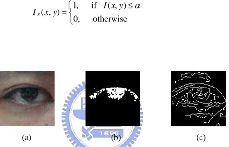
An intensity field I and an edge field s E are given by a threshold s α according as the low intensity of iris and highly contrast between iris and sclera respectively. Edge field is produced by Canny edge operator and intensity field shows below. 1, if ( , ) ( , ) 0, otherwise s I x y I x y = ⎨⎧ ≤α ⎩ (3.9) (a) (b) (c)

Fig. 3.2 An eye region image of edge field and intensity field. (a) Input image. (b) Intensity field. (c) Edge field.

Observe the region of iris in Fig. 3.2(b), we find out there are some small holes in this region because of the variation or noise corruption and the intensity field is not suitable for template search. Using this intensity field for estimate the maximum intensity region will not work reliably. This is because that the uneven intensity distribution accounts for the wrongly convergence in template fitting. On the other hand, on observing Fig. 3.2(c), there are too many edges are answer to use edge field Circle template commonly observed both in Figs. 3.2(b) and 3.2(c), could be helpful for iris search. Accordingly, we must modify this approach obtain color compensating

procedure for intensity field. Do Canny edge operator in intensity field image which has been color compensated instead of input eye image.

3.5.2 Anisotropic Diffusion

The approach we proposed to compensate the input eye image for intensity field is anisotropic diffusion. In [22], Black mentioned diffusion algorithms could remove noise from an image by modifying the image via a partial differential equation (PDE). For example, consider applying the isotropic diffusion equation (the heat equation) given by ∂I x y t

(

, ,

)

/ = div∂t

( )

∇I , using the original (degraded/noisy) image

(

, , 0

)

I x y as the initial condition,

( )

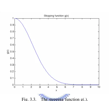
x y, specifies spatial position, t is the number of iteration, and where ∇I is the image gradient. Modifying the image according to this isotropic diffusion equation is equivalent to filtering the image with Gaussian filter; however it result in blurring the edge.

Perona and Malik [23] proposed the anisotropic diffusion equation as follows:

( )

= div

t

I ⎡_⎣g ∇ ∇I I⎤_{⎦ (3.10)}

where ∇I is the gradient magnitude, and g

( )

∇I is an “edge-stopping” function. This function is chosen to satisfy g x

( )

→ 0 when x → ∞ so that the diffusion is “stopped” across edges as Fig. 3.3. The “edge-stopping” function is adopted in [25] are

( )

(

( I /K)2

)

and

( )

1 ₂ 1 g I I K ∇ = ⎛ ∇ ⎞ + ⎜ ⎟ ⎝ ⎠ . (3.12)

Fig. 3.3. The stepping function g(.).

The constant K was fixed either by hand at some fixed value, or using the “noise estimator” described by Canny [24].

Perona and Malik discretized their anisotropic diffusion equation as follows:

(

)

1 , , s t t s s s p s p p I I g I I η λ + ∈ = +

∑

∇ ∇ (3.13)

where Ist is a discretely sampled image, s denotes the pixel position in a discrete, two-dimensional (2-D) grid,, t now denotes discrete time steps (iterations), and

determines the rate of diffusion, η represents the spatial neighborhood of pixel s, s

and η is the number of neighbors (usually four, except at the image boundaries). s

Perona and Malik [23] linearly approximated the image gradient (magnitude) in a particular direction as

, t,

sρ ρ s ρ ηs

∇Ι = Ι − Ι ∈ . (3.14)

We show the local neighborhood of pixels at a boundary in Fig. 3.4. Fig. 3.5 shows the example of the noise image and its result image after anisotropic diffusion processing.

Fig. 3.4. Local neighborhood of pixels at a boundary (intensity discontinuity).

(a) (b) (c)

Fig. 3.5. A diagram of anisotropic diffusion algorithm. (a) The noisy image. (b) The processed image after average mask. (c) The image after anisotropic diffusion.

(a) (b)

Fig. 3.6. An eye image after anisotropic diffusion. (a) Input image. (b) Output image.

(a) (b) (c)

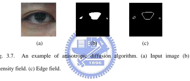
Fig. 3.7. An example of anisotropic diffusion algorithm. (a) Input image (b) Intensity field. (c) Edge field.

The effect of noisy artifact removal by is illustrated below. After anisotropic diffusion procedure on Fig 3.6, we got an eye region image with the iris and the rest smoother distribution of intensity. Uniform intensity field is helpful for the template search, which is due to a smooth average intensity amount for the iris candidate regions. In the edge field, the remainder edges out of rounded boundary ones have been discarded, thus we can find the correct iris circle handily.

Here is another problem that the edge sometimes shrinks to the small region inner the iris as shown in Fig. 3.8(b). From this figure, it is easy to en-circle the small region with the dark intensity, which has some edges are formed by upper eyelid and iris. This wrong encircling can be avoided by the following: First, we

eliminate the horizontal edges as shown in Fig. 3.8(f). Then a circle coincides with most of the edge detected is the good candidate for iris. The result with imposed circle for iris is shown in Fig. 3.8(e).

(a)

(b) (c) (d)

(e) (f) (g)

Fig. 3.8. Eliminating the horizontal edges of (c) produces (f). (b) is invalid result. (e) is valid result.

3.5.3 Circular Deformable Template

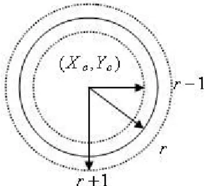
An adaptive search region from PCA algorithm and better edge field and intensity field by Section 3.5.1 and 3.5.2 help to do the template search task. Then, we set up the circular template subsequently, which require only two parameters. In this way we can simplify the template model and thus reduce template searching time. The circular template model is composed of the radius r and the center point (Xc,Yc)

as shown in Fig. 3.9. Considering the iris is not precise round, there is a range from 1

radius r for fitting intensity.

Fig. 3.9. The diagram of circular template model.

According to the color and shape characters of the iris, its low intensity value and round edge are located to iris. To this setting, shift the circle center pixel by pixel in the search region of the eye which is chosen from PCA and then record the cumulative intensity value P and cumulative edge number I P , defined below: E

( , ) ( , ) 1 ( , ) ( , , ), 1, , [0, 1]. C c c I c c s I C x y A X Y P X Y I x y r r M P A _∈ =

∑

= ∈ (3.15) ( , ) ( , ) 1 ( , ) ( , , ), 1, , [0, 1]. C c c E c c s E C x y L X Y P X Y E x y r r M P L _∈ =

∑

= ∈ (3.16)

where A and c L are the area and circumference of the deformable circle. c Deformable circle’s radius r ranges from 1 to the height N of the rectangular eye region.

These two characters of iris favor circular template and we obtain the best circle of iris by :

{

}

, , ,

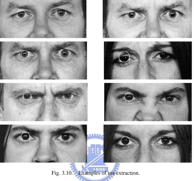
Based on the proposed scheme above, some experimental iris extraction are shown below. The input image samples are obtain from FACS database at http://face-and-emotion.com/.

Fig. 3.10. Examples of iris extraction.

Chapter 4 Eye State Determination

4.1 Analyzing the Iris Region

After the iris extraction and circular deformable template search mentioned in Chapter 3, we subsequently can analyze the iris image. The iris is a circular and dark colored region on the eyeball. The color of the iris is mainly determined by the reflection of environmental illumination and the iris’ texture and patterns including the pupil (an aperture in the center of the iris) [25].

Referring to Fig 4.1, human eye closeness state can be simplified to the observable ratio of iris. When human blink his eyes, the eyelid covers the iris and the observable ratio of iris is defined to be the ratio of dark area to the whole iris region. This ratio, as shown in Fig 4.2, will change momentarily when someone blinks his eyes or close them. However, it is difficult to measure the observable ratio of the iris exactly, particularly the closing eye state. Because of there exists many interferences like eyelashes and deep eyelid fold, these makes the iris region noisy and difficult to detect accurately. In practice, we frequently need detect the drowsy state of a person, in this case we just need to know the observable ratio of the iris, which simplifies the task to some extent. The reason why will be is described in the next section.

Fig. 4.1. Physiological motion of human eye.

Fig. 4.2. Observable ratio of the iris appearance.

4.2 Determining Eye State

When someone falls asleep or fatigues, his eyelid will rise and fall with an increasing frequency in the beginning and his eye stays barely open during drowsy. With this fact in mind, we estimate the eye closeness into three states: open, barely open and closed; instead of just open and closed states.

The observable ratio of iris in normal (open) state is different among people. Someone open his eye with iris in totally seen scale but others open his eye with iris covered by upper eyelid to some extent. To this fact, determining one’s eye opened state should also consider his eye open/closed habit. Namely, we have to know the commonly observable portion of the iris, which specifies his normal (open) state of the eye. Firstly, the tester keeps his eyes in open state and the system counts his observable portion of irisI by t

, ( , ) ( ) ( , ) c c c t s x y A X Y I I x y ∈ =

∑

(4.1)

Where is center point of the output solution after template search. Three states of open, barely open and closed are defined as follows:

0.6, Open state. 0.2 0.6 Barely open state.

0.2 Close state. s t S t s t I I I I I I ⎧ ≥ ⎪ ⎪ ⎪⎪ _{< <} ⎨ ⎪ ⎪ ≤ ⎪ ⎪⎩

∑

∑

∑

(4.2)

A problem often encountered when the eye is in almost close, in which the iris is almost completely covered by the eyelid. Our system still output an image and the intensity value as the eye image. According to our experience, we found that our imposed circles will be located around the eye inner corner principally. This is because that eye corner contains low intensity and edges comparatively. Our iris imposed circle is liable to locate the barely open or open eyes, and is not reliable for closed eye. To solve this problem, we have to resort to the image’s HSI color domain and utilize the hue component as a reference.

Fig 4.3 shows the eye state from open to completely closed, the hue images in the right column, decrease their values when the eye changes from open to closed. With this observation in mind, and we add an extra criterion based on eye’s hue component of an eye image. If the hue ratio is lower than 50% of its normal (open) state, the eye is classified to closed state no matter what the observable ratio of the iris is.

4.3 Drowsy State Detection

Of the drowsiness detection measures and technologies evaluated in various studies, the measure referred to as “PERCLOS” was found to be the most reliable and valid determination of a driver’s alertness level. PERCLOS is the percentage of eyelid closure over the pupil over time and reflects slow eyelid closures (“droops”) rather than blinks. A PERCLOS drowsiness metric was established in a 1994 driving simulator study as the proportion of time in a minute that the eyes are at least 80 percent closed.

Eyelid closure has been recently proven to be a very reliable and meaningful indicator of drowsiness while driving. Wierwille et al. [3] found that it is indicative of a subject at the onset of drowsiness leading to poor response. If a driver’s eyelids are closed during driving, his ability to operate a vehicle would be greatly hampered. The researchers demonstrated that PERCLOS, defined as the proportion of time that the eyes of the subject are closed over a specified period, can be used as a physiological indicator of drowsiness. Accordingly, a subject can be said to be drowsy if he has a high PERCLOS value. For example, suppose the eye of one subject is detected to be in the closed state, 80% closed as defined previously, for six seconds within one minute. The PERCLOS will be 6/60 = 10%. That is, the subject closes his eyes in 10% of one minute. Our proposed system would be a useful component to PERCLOS estimation.

Fig. 4.4. Flowchart of eye openness state detection system. Input image

(frontal view)

Face segmentation

Detect eye region by PCA

Deformable template search

Determine eye state

Chapter 5 Experimental Result

5.1 Experiment Setting

To examine our proposed algorithms, experiments with different face image sequences were collected. The input image sequences are captured under ordinary daylight illumination and the images are nearly frontal-view faces and the faces do not have movement or a little movement in face plane. Our testing images are 640*480 facial color images. Our test images contain 50 images per each tester on a 3.2 gigahertz PC and the algorithm programmed in MATLAB. The initial condition

t

I was determined firstly from the tester opened his eye in normal state. Thus we can

calculate the thresholds for eye state classification. Some experiment results of different testers are shown in Figs. 5.1－5.4. In these figures, column (a) is composed

of eye region of face images; column (b) is anisotropic diffusion; the intensity field images are shown in column (c), and the edge field images are shown in column (d). The ground truth was built manually. Namely, we extracted the best fitting iris image by hand and then calculated observable ratio by image processing software. Then calculated the thresholds for eye state classification and classified the input images into three eye openness states by Eq. (4.2).

5.2 Experiment Result (a) (b) (c) (d)

Fig. 5.1. Different observable ratio of the iris of Sample 1. (a) Input images, with detected iris circle imposed. (b) The images after anisotropic diffusion. (c) The intensity field. (d) The edge field.

(a) (b) (c) (d)

Fig. 5.2. Different observable ratio of the iris of Sample 2. (a) Input images, with detected iris circle imposed. (b) The images after anisotropic diffusion. (c) The intensity field. (d) The edge field.

(a) (b) (c) (d)

Fig. 5.3. Different observable ratio of the iris of Sample 3. (a) Input images, with detected iris circle imposed. (b) The images after anisotropic diffusion. (c) The intensity field. (d) The edge field.

(a) (b) (c) (d)

Fig. 5.4. Different observable ratio of the iris of Sample 4. (a) Input images, with detected iris circle imposed. (b) The images after anisotropic diffusion. (c) The intensity field. (d) The edge field.

It is to be noted from Fig. 5.1(a) that the eye images of tester 1 contain his eye images from open to barely open, and finally to closed states, so to Figs. 5.2(a)－Figs.

5.4(a). Figs. 5.5(a)-5.5(d) shows the observable ratio of the iris in L1 and the hue ratio, in L2 for Figs. 5.1(a)－5.4(a), respectively. The observable ratio of the iris of open

state is setting upper than 60%, the barely open state is between 60% and 20%, and the closed state is lower than 20%. When the hue ratio, the cumulative hue values of pixels to the cumulative hue values of pixels in normal open eye state, ten sample is lower then 50%, the eye image was classified to closed state no matter what the observable ratio of the iris is, see image of Fig. 5.5(a). At last, the accuracy of three states is 98%, 86%, and 97% for open state, barely open state, and closed state respectively. Total average accuracy of three states is 94%.

Sample 1 0 20 40 60 80 100 120 1 2 3 4 5 6 7 8 9 10

Input image index

R atio % L1 Iris L2 Hue (a)

Sample 2 0 20 40 60 80 100 120 1 2 3 4 5 6 7 8 9 10

Input image index

Ra ti o % L1 Iris L2 Hue (b) Sample 3 0 20 40 60 80 100 120 1 2 3 4 5 6 7 8 9 10

Input image index

R atio % L1 Iris L2 Hue (c)

Sample 4 0 20 40 60 80 100 120 1 2 3 4 5 6 7 8 9 10

Input image index

R atio % L1 Iris L2 Hue (d)

Fig. 5.5. Observable ratio of the iris (L1) and hue ratio of the eye region (L2). (a) Correspond to Fig. 5.1. (b) Correspond to Fig. 5.2. (c) Correspond to Fig. 5.3. (d) Correspond to Fig. 5.4.

TABLE II

Accuracy of three eye states detection

Open Barely open Closed

Number Accuracy % Number Accuracy % Number Accuracy % Sample 1 24 92 23 87 3 100 Sample 2 8 100 34 82 8 100 Sample 3 9 100 36 89 5 90 Sample 4 3 100 43 84 4 100 44 98 136 86 20 97 Total

Chapter 6 Conclusions and Future Work

In this thesis, we have proposed an algorithm for the eye openness state detection. We have obtained a satisfactory accuracy of three openness states, including open, barely open, and closed states. But there still have many problems to be overcome, such as the input images captured in the night. In these case, we could utilize infrared camera to capture the image or by other approaches. The other problem is the head movement, which can lead to wrong frontal face image and locate the eye region detection.

An eye state detection system application in drowsy detection can help a driver avoid the accident caused from his fatigue. This system is simple and hence suitable to be a key component of real-time drowsy state detection system. It is sure that the accidents can be detracted by applying the drowsy state detection system.

References

[1] A. Yuille, P. Hallinan, and D. Cohen, “Feature Extraction from Faces Using Deformable Templates,” International Journal of Computer Vision, vol. 8, no. 2, pp. 399–111, 1992.

[2] J. Deng and F. Lai, “Region-Based Template Deformation and Masking for Eye-feature Extraction and Description,” Pattern Recognition, vol. 30, no. 3, pp. 403–419, March 1997.

[3] W.W Weirwille., “Overview of Research on Driver Drowsiness Definition and Driver Drowsiness Detection,” in Proc. 14th International Technical Conference on

Enhanced Safety of Vehicles, pp. 23-26, Munich, Germany, May, 1994.

[4] E. Hjelmas and B. K. Low, “Face detection: A survey,” Computer Vision and Image

Understanding, vol. 83, pp. 236–274, 2001.

[5] R. Feraud, O. J. Bernier, J. Viallet, and M. Collobert, “A Fast and Accurate Face Detector. Based on Neural Networks,” IEEE Trans. Patt. Anal. Machine Intell., vol. 23, no. 1, January 2001.

[6] D. Maio and D. Maltoni, “Real-time face location on gray-scale static images,”

Pattern Recognition, vol. 33, pp. 1525–1539, 2000.

[7] C. Garcia and G. Tziritas, “Face detection using quantized skin color regions merging and wavelet packet analysis.” IEEE Trans. Multimedia, vol. 1, no. 3, pp. 264-277, 1999.

[8] H. Wu, Q. Chen, and M. Yachida, “Face detection from color images using a fuzzy pattern matching method,” IEEE Trans. Patt. Anal. Machine Intell., vol. 21, pp. 557–563, 1999.

44

[9] H. Rowley, S. Baluja, T. Kanade, “Neural network-based face detection.” IEEE

Trans. Patt. Anal. Machine Intell., vol. 20, no. 1, pp. 23－38, 1998.

[10] K. Sung and T. Poggio, “Example-based learning for view based human face detection. ” IEEE Trans. Patt. Anal. Machine Intell., vol. 20, no. 1, 39－51, 1998.

[11] M. Yang and N. Ahuja, “Detecting human faces in color images.” in Proc. IEEE

Conference on Image Processing, Chicago, pp. 127－139, 1998.

[12] A. Colmenarez and T. Huang, “Face Detection with Information-Based Maximum Discrimination.” in Proc. IEEE Conference on Computer Vision and Pattern

Recognition, San Juan, PuertoRico, 782–787, 1997.

[13] K.C. Yow and Cipolla, “Feature-Based Human Face Detection,” Technical Report

CUED/F-INFENG, TR 249, Dept. of Eng., Univ. of Cambridge, England, 1996.

[14] M. S. Lew and N. Huijsmans, “Information Theory and Face Detection,” in Proc.

13th International Conference on Pattern Recognition (ICPR'96), Vol. 3, pp.

601, 1996.

[15] G. Donato, M. S. Bartlett, J. C. Hager, P. Ekman, and T. J. Sejnowski, “Classifying facial actions,” IEEE Trans. Patt. Anal. Machine Intell., vol. 21, no. 10, pp. 974–989, October 1999.

[16] J. Huang and Y. Wang, “Compression of color facial images using feature correction two-stage vector quantization Image Processing,” IEEE Trans. Image Processing, Vol 8, no. 1, pp. 102–109, Jan. 1999.

[17] D. Chai and K. N. Ngan, “Face segmentation using skin-color map in videophone applications,” IEEE Trans. Circuits Syst. Video Technol., vol. 9, pp. 551–564, 1999. [18] T. Kurozumi, Y. Shinza, Y. Kenmochi, and K. Kotani, “Facial individuality and

expression analysis by eigenspace method based on class features or multiple discriminant analysis,” in Proc. International Conference on Image Processing, vol. 1, pp. 648–652, 1999.

[19] M. Turk and A. Pentland, “Eigenfaces for recognition,” Journal of Cognitive

Neuroscience, vol. 19, pp. 743–756, 1997.

[20] L. H. Staib and J. S. Duncan, “Boundary finding with parametrically deformable models, ” IEEE Trans. Patt. Anal. Machine Intell., vol. 14, no. 11, pp. 1061–1075, 1992.

[21] M. P. D. Jolly, S. Lakshmanan, and A. K. Jain, “Vehicle segmentation and classification using de-formable templates,” IEEE Trans. Patt. Anal. Machine Intell., vol. 18, no. 3, pp. 293–308, 1996.

[22] Harris and M. Stephens, “A combined corner and edge detector,” in Proc. 4th Alvey

Vision Conference, pp. 147–151, 1988.

[23] Perona and J. Malik, “Scale space and edge detection using anisotropic diffusion,”

IEEE Trans. Pattern Anal. Machine Intell., vol. 12, no. 7, pp. 629–639, July 1990.

[24] Canny, “A computational approach to edge detection,” IEEE Trans. Patt. Anal.

Machine Intell., vol. 8, no. 6, pp. 679–698, Nov. 1986.

[25] T. Moriyama, T. Kanade, J. Xiao, and J. Cohn, “Meticulously Detailed Eye Region Model and Its Application to Analysis of Facial Images,” IEEE Trans. Patt. Anal.