An Implementation of Distributed Framework of Artificial Neural Network for Big Data Analysis

DOI: 10.6245/JLIS.2016.422/656

An Implementation of Distributed Framework

of Artificial Neural Network for Big Data Analysis

Jiing-Yao Chang

Chief of Teaching and Research Section, Computer Center

Adjunct Assistant Professor, Department of Management Information Systems, National Chengchi University, Taiwan (R.O.C.)

E-mail: [email protected]

Wen-Ching Liou Associate Professor,

Department of Management Information Systems, National Chengchi University, Taiwan (R.O.C.) E-mail: [email protected]

Shan Hao Ho

Master Student, Graduate institute of Management Information Systems, National Chengchi University, Taiwan (R.O.C.)

E-mail: [email protected]

Keywords: Artificial Neural Network; Big Data Analysis; Data Mining; Distributed Computing; Multilayer Perceptron

【Abstract】

In this research, we introduce a distributed framework of artificial neural network (ANN) to  deal  with  the  big  data  real‐time  analysis  and  return  proper  outcomes  in  very  short  delay.  The  result of our experiment shows that training the distributed ANN model could be converged in 17  seconds  on  24‐core  clustering  platform  and  learns  that  multi‐model  with  stratification  strategy  would obtain most true positive predictions with nearly 70% precision at voting threshold value  equal to 0.7. 

In our system, ANNs are used in the data mining process for identifying patterns in financial  time series. We implement a framework for training ANNs on a distributed computing platform. 

We  adopt  Apache  Spark  to  build  the  base  computing  cluster  because  it  is  capable  of  high  performance  in‐memory  computing.  We  investigate  a  number  of  distributed  back  propagation  algorithms and techniques, especially ones for time series prediction, and incorporate them into  our framework with some modifications. With various options for the details, we provide the user  with flexibility in neural network modeling. 

Introduction

Generally, there are four phases: generation, acquisition, storage and analysis in the valued chain of big data. Big data analysis is the final and important one which provides decision making and brings benefits to organizations and individuals through rapid extraction of valued information from the massive data (Padgavankar & Gupta, 2014). It is perhaps the one attracting most attention in recent years. In our research, data from financial institute are varies by time and huge volume, so as to be able to categorized as real-time and massive level analysis (Chen, Mao, Zhang, & Leung, 2014). Such analysis process is a problem with high complexity. In this research we approach the problem with artificial neural network (ANN) which is known as one of the methods suitable for complex problems solving.

Strategy Planning with Artificial Neural Network

An artificial neural network, or simply a neural network, is an information processing paradigm inspired by central nervous systems of animals and is capable of machine learning and pattern recognition. Like a biological neural system, an artificial neural network consists of multiple interconnected neurons which receive and process input signals to produce output signals. A trading strategy, in our definition, is a mathematical model which takes the values of quotes and financial indicators at a specific time point as the variables and, though computation, produce a trading signal as the output. Hence in this context, the input of the neural network is quotes and indicators, and the output is a trading signal.

In this research, we adopt a commonly used model of feedforward ANN known as multilayer perceptron (MLP) which uses backpropagation algorithm for learning. In the backpropagation algorithm, a training pattern in the training set is a pair of an input vector and an output vector. Hence in this context, the input vector of a training pattern contains quotes and indicators at a specific time point, and the output vector contains a trading signal at the same time point. Consequently, the training set will be a time series. Learning of an MLP is the adaptation of

weights (multiplication effect applied to input) in the network. An MLP consists of multiple layers; each layer consists of multiple neurons; each neuron holds a weight vector. Therefore, an MLP trading strategy can be represented as a mathematical model with the network structure as the function, quotes and financial indicators as the variables, and a third-order tensor of weights (or a weight tensor) as the coefficients.

Training ANNs on a Distributed Computing Platform

The training process of neural networks is usually time- and CPU-consuming, especially when using a large volume of time series data. For performance, scalability and fault tolerance, we decide to train our neural networks distributed. Instead of the renowned Hadoop MapReduce, we choose to adopt Apache Spark to build the base computing cluster because it is able to execute distributed tasks in memory (avoiding overheads of disk I/O) and promises up to 100 times the performance of Hadoop MapReduce (Xin et al., 2013). It has also been proven that Spark is highly scalable with the cluster size of 100 nodes in the lab (Zaharia et al., 2012) and 80 nodes in production at Yahoo (Feng, 2013). Hence in this research, we propose a distributed framework of artificial neural network for big data analysis on financial time series prediction.

Literature Review

Time Series Prediction with ANN

The application of artificial neural networks in predicting time series data can be traced back to late 1980s. The research of White (White, 1988) presents a method to identify patterns in asset price movements with neural networks. Although the author considers the result as a failure, his research provides some valuable insights and modifications to contemporary machine learning techniques.

Jones et al. (Jones et al., 1990) uses neural networks for function approximation and the time series prediction. They propose an improved learning algorithm which is able to reduce size of training set while maintaining the performance of a network with linear weights.

Kimoto, Asakawa, Yoda and Takeoka (Kimoto, Asakawa, Yoda, & Takeoka, 1990) present a TOPIX (Tokyo Stock Exchange Prices Indexes) prediction system based on neural network. Into the system they incorporate some improvements to the learning process of neural network, including a modified backpropagation algorithm and the moving window (or sliding window)

technique for selecting training sets. The system exhibits excellent results in trading simulation. When comparing to multiple regression analysis, the neural network produces a much higher correlation coefficient.

Kaastra and Boyd (Kaastra & Boyd, 1996) provide a practical introductory guide to the design of a neural network for forecasting financial and economic time series. An eight-step procedure focusing on backpropagation neural network is defined as follows.

1. Variable selection: The researcher must decide the input of the network by choosing which indicators to use. It depends on the research objectives that whether to use technical indicators, fundamental indicators or both and what the frequency of data should be.

2. Data collection: When collecting data, the researcher must consider cost, availability, reliability of the data source, consistency in the calculation over time, etc.

3. Data preprocessing: The input and output are rarely fed into the network in raw form. It is crucial to analyze and transform the data in order to minimize noise, highlight important relationships, detect trends, and flatten the distribution.

4. Training, testing, and validation sets: Common practice is to divide the time series into training, testing, and validation sets. There are different methods to determine these three sets. A rigorous approach is to use moving window testing.

5. Neural network paradigms: An improperly constructed neural network could cost more time and computing power without producing better results. It is important to properly determine appropriate number of layers, number of neurons of neurons in each layer, and transfer function.

6. Evaluation criteria: There are various error functions which can be used for evaluation. The most common one minimized in neural networks is the sum of squared errors.

7. Neural network training: A neural network learns by iteratively processing examples and adjusting its weights. Properly assigned number of epochs (an epoch is an iteration of presenting all training data to the network) and value of learning rate and momentum can ensure performance and the chance the reach global minimum of error.

8. Implementation: The environment in which the neural network will be deployed requires careful consideration. Also, deployed networks needs periodic retraining to maintain their performance.

In addition to the steps above, the authors also list some key factors to successful application. Fortunately, with a self-developed system, such requirements are not difficult to achieve in our research.

Distributed Backpropagation Algorithm

One way to execute backpropagation distributed is to partition neurons into several disjoint subsets and assign them to different processors or computing nodes in the distributed system. Each processor/node processes its local neurons and passes on the outputs to neurons in the next layer by communicating with other processors/nodes. There are two schemes of partitioning called vertical partitioning and hybrid partitioning (Ganeshamoorthy & Ranasinghe, 2008; Sudhakar & Murthy, 1998; Suresh, Omkar, & Mani, 2005; Yoon, Nang, & Maeng, 1990). While hybrid partitioning is claimed as improving performance over vertical partitioning by reducing computation and communication overheads, the network still needs frequent communication. Therefore, the neuron parallelism is considered to be suitable for systems with low inter-processor communication costs. The communication overheads would be overwhelming if we implement neuron parallelism on a computing cluster.

Another type of parallelism is called training pattern parallelism (Andonie, Chronopoulos, Grosu, & Galmeanu, 1998; Dahl, McAvinney, & Newhall, 2008; Gu, Shen, & Huang, 2013; Liu, Li, & Miao, 2010; Pethick, Liddle, Werstein, & Huang, 2003). The neural network will not be partitioned across the cluster; instead, it is copied onto nodes in the cluster. Each node maintains a clone of the neural network, learns a subset of the whole training set and returns its local weight deltas which are later aggregated.

Various techniques for constructing subsets have been proposed. The most straightforward one is to divide the training set into disjoint subsets by the number of worker nodes. The system in the research of (Gu et al., 2013) is implemented in this way and the partitions are kept static, i.e., each node holds its designated subset throughout the entire training process. The advantage of static partitioning is that subsets can be cached locally on their corresponding nodes to increase performance. Dahl et al. (2008) use a technique of random sampling to avoid possible anomalies cause by predefined ordering of the data. In their algorithm, each node is presented with a randomly sampled subset of a certain size every epoch. A potential problem of random sampling is that each patterns might not be presented to the neural network with the same number of times, allowing the possibility of sampling bias.

The frequency of updating weights is also varied. In the standard backpropagation algorithm, weights can be updated after each presentation of pattern or at the end of an epoch (Pethick et al., 2003). In a distributed algorithm, it is preferable to commit a batch update at the end of each epoch to reduce communication overheads. Each clone accumulates its own set of local weight deltas and returns it to the master node. Weight deltas of all clones are aggregated by taking either sums or averages, and updated into the weights on the original instance of the neural network on the master node (Andonie et al., 1998; Gu et al., 2013; Liu et al., 2010). A hybrid technique is used in the algorithm proposed by Dahl et al.(Dahl et al., 2008).The local weights on each node are updated on a per-pattern basis in order to support the momentum term in the delta function. At the end of each epoch, the weights are updated in batch with local weight deltas from all nodes.

Technologies for Parallel and Distributed Computing

To implement the framework (and the underlying system of course), we consider some criteria such as performance, scalability, and fault tolerance. Based on the criteria, we have surveyed a number of software technologies.

We use the programming language called Scala mainly because it supports concurrency and data parallelism on language level (in contrast to the API-level support for which in Java). The feature makes it easier to develop and maintain modules for parallel tasks which fully utilize multi-core processors of modern computers. Another good reason for using Scala is the ability to integrate with Java seamlessly (“Scala Documentation”, n.d.).

As mentioned above, we adopt Apache Spark for our computing platform. The core concept of Spark is Resilient Distributed Dataset (RDD), a distributed memory abstraction enables in-memory distributed computations and is fault-tolerant (Zaharia et al., 2012). It has been proven to be suitable for a number of applications including machine learning. It also provides native support for the Scala language.

Considering concepts and technologies above, in our framework, Spark is used to address parallelism across the computing cluster, and Scala is used to address parallelism within one computing node.

Distributed Framework of ANN

In this section, the data mining process we followed, conceptual model and architecture of the distributed framework of ANN will be introduced.

Data Mining Process in Big Data Analysis

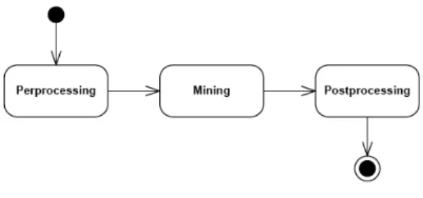
The distributed framework of ANN is used as one of the data mining algorithms in the big data analysis phase. The data mining process is composed of three stages, as illustrated by the UML activity diagram in Figure 1. The input is the financial time series data with configuration parameters of ANN model and the output is the suggested trading strategy along with its backtesting result. Each stage contains a few steps explained as follows.

Figure 1 Data Mining Process

Preprocessing

There are three steps in this stage, namely gathering, signalizing and transforming, as explained below.

1. In step one, the time series of financial indicators used for mining is gathered from the database based on the user’s selection of investment object, technical analysis indicators (TAIs) and time intervals.

2. In step two, the time series of financial indicators is used to compute target trading signals at each time point, resulting another time series of signals. The two sets of time series is the mapped into a training set, a time series of indicators-signal pairs.

3. In the optional step three, the training set is transformed with one of the techniques including normalization, first differentiating or natural log as specified by the user.

Consequently, this stage is where step three (data preprocessing) of the guide by Kaastra and Boyd (1996) is mainly addressed.

Mining

In this stage, the algorithm along with algorithm-specific parameters set by the user is executed on the training set prepared in the previous stage. In the case of the ANN algorithm, step

four to seven (training, testing, and validation sets; neural network paradigms; evaluation criteria; neural network training) of the guide by Kaastra and Boyd (1996) is addressed—with one exception. The validation set is not of consideration in this stage.

Postprocessing

There are two steps in this stage, namely formulating and backtesting, as explained below. In step one, a trading strategy is formulated as a mathematical model with indicators as the variables and output of the mining algorithm as the function and coefficients.

In step two, the formulated strategy is put to backtesting on the simulation set specified by the user. The strategy and the backtesting result consists the output of the data mining task.

The gathering of the simulation set is also the last piece of step three (data preprocessing) of the guide by Kaastra and Boyd (1996) and the simulation set is effectively the validation set from step four (training, testing, and validation sets) of the guide.

In the system, stage one and stage three are handled by shared modules. In other words, all mining algorithms can depend on the same modules for preprocessing and postprocessing. Some algorithms might have needs for data transformation for better result. We provide options and suggestions on the GUI while leaving the decision to the user.

Conceptual Model of the Distributed Framework of ANN

After the data mining process explained, the distributed framework of artificial neural network can be introduced. In the framework, we adopt a commonly used model of feedforward ANN known as multilayer perceptron (MLP) which uses a supervised learning algorithm called backpropagation for learning. The training set used in backpropagation is from the output of the preprocessing stage, a time series of training patterns (indicators-signal pairs). The training set is divided into a learning set and a testing set. The learning set is used for the MLP to learn—to adapt its weights in order to minimize the error between actual output signals and target signals. The testing set is used to test if the error is minimized.

In our definition, the trading signal in a training pattern is either zero or one, where a signal of one suggesting either to take an action of buying or selling depending on the strategy configuration, and a signal of zero suggesting no action should be taken. Pattern with the target signal of one in a training set is usually of a small portion. In other words, most signals would be zero, which might

affect the mining algorithm by over-emphasizing signals of zero. In contrary, the objective of a mining algorithm is to find reliable signals of one. Because of this characteristic in the training set, there are two different paradigms of model building tasks for mining algorithms, namely single-model task and multi-model task. The single-model task takes the whole training set as the input and return one trained model. The multi-model task takes a collection of subsets, each of which is composed of all patterns with signal of one and a part of patterns with signal of zero, as illustrated in Figure 2.

Figure 2 Training Set and Training Subsets

In the single-model training session, the algorithm would have pattern-level parallelism. On the other hand, in the multi-model training session, the algorithm adopts perceptron-level parallelism (or network-level parallelism), where each training subsets is learned by one MLP and multiple MLPs are processed simultaneously and independently (Ho, 2014).

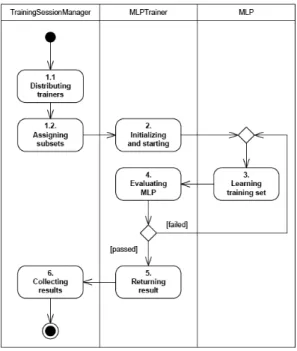
In this paper, we will focus on introducing multi-model algorithm which might take most parallelized and more efficient on big data analysis. The multi-model training session can be modeled by the UML activity diagram in Figure 3.

The multi-model training session realize distributed computing with perceptron-level parallelism across worker nodes among the cluster. This is in practice less complicated than the single-model because it uses only traditional backpropagation algorithm. Each perceptron is trained independently. No communication is need during the training process. The weights are updated on a per-pattern basis. The result of a multi-model session is a collection of the results from all trainers. The steps of the multi- model training session are explained as follows.

Figure 3 Multi-model Training Session

Step 1: Distributing and assigning. A multi-model training session receives a collection of training subsets as the input. For each subset, an MLP trainer is created to train an instance of plain, simple MLP. These trainers are then distributed across the cluster to process their own subsets respectively.

Step 2: Initializing and starting. This step is the same as the step two of a single- model session. From the perspective of a trainer, there is no difference between a simple MLP and a distributed MLP.

Step 3: Learning training set. The simple MLP is presented with the learning set once. The MLP learns by backpropagation with momentum, updating weights on a per- pattern basis. A part of step seven (neural network training) of the guide by Kaastra and Boyd (1996) is addressed here.

Step 4: Evaluating MLP. Since there is no difference between a simple MLP and a distributed one from the perspective of a trainer, this step is the same as the step five of a single-model session.

Step 5: Returning result. For the same reason, this step is also the same as the step six of a single-model session.

Step 6: Collecting results. The results from all trainers are gathered—not aggregated—into a collection and returned as the result of the multi-model session. The result will be converted into a multi-model strategy in the postprocessing stage. A multi-model strategy processes the input vector with all models and decides the final output signal by voting.

Architecture of the Distributed Framework of ANN

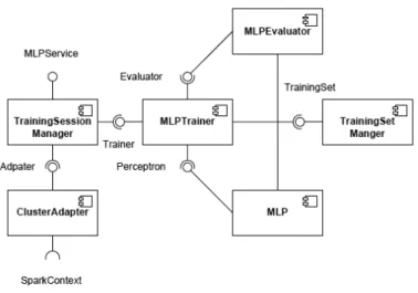
The architecture of the distributed framework of ANN is designed to be object- oriented and can theoretically be implemented using any object-oriented programming language. In this research we implement it with Scala. The design is based on the real world analogy that the trainer teaches the learner and the learner is tested by the evaluator to determine the result of learning. The components and their relationships would be illustrated in Figure 4.

Figure 4 Components for Multi-model Training Session

In the distributed algorithm, which is depicted in Figure 3, the learning process is actually performed by multiple learning units, but in the architecture they are wrapped into one to simplify the relationship between components. In addition, a training set manager is designed for handling the training set. The components used in multi- model training session are mostly the same as which in signal-model session (Ho, 2014). The differences are that the simple MLP is used instead of the distributed MLP and the training session manager connects to the cluster.

TrainingSessionManager: This component works as the entry point of the framework. It performs the same three functions as in a single-model session, but with slight differences.

Instantiation: The same as in in a single-model session.

Starting: In a multi-model session multiple trainers and perceptrons are created. Trainers are distributed across the clusters and therefore the training session connects to the cluster through the adapter.

Completion: Once the trainer finishes training, the training session manager collects information from all trainers, composes a collection of simulation results and returns.

ClusterAdapter: This component initializes an instance of SparkContext and connects to a Spark cluster. Theoretically we can connect to different distributed computing platform by replace the adapter.

MLPTrainer: The trainer works as the coordinator during the training process. It works the same as in a single-model session since both the simple MLP and the distributed MLP implements the interface (trait in Scala) of Perceptron.

TrainingSetManager: The training set manage provides access to the training set. It works the same as in a single-model session. The only difference is that an instance of training set manager handles only one training subset.

MLPEvaluator: The evaluator tests the perceptron with the training set. It works the same as in a single-model session.

MLP: The plain, simple MLP which learns locally on one computing node. It performs four major functions, namely construction and learning, as explained below.

1. Construction: This component constructs itself with parameters received.

2. Learning: This component learns a learning set by the backpropagation (with momentum) algorithm.

Experiments

Training Time Experiment Method

To analyze the performance of the distributed framework of ANN we designed the following experiment. The distributed framework is deployed on a cluster of desktop computers (each with a PC-class quad-core CPU and 4 GB of RAM).

Input data: The TAIs of in our system is generated every second. In other words, a training set is a time series of training patterns with the interval of one second. In the experiment, we use one trading day (about 18,000 seconds) of training patterns as the training set. As mentioned previously, there two types of training session, and therefore the experiment of training time is made on the single-model training session and the multi-model training session respectively.

Independent variables: A worker node is a quad-core PC. To analyze the performance, we adjust the number of worker nodes (i.e. the number of cores) used for training. It is possible to use

part of one worker node’s resources (e.g. two cores or three cores) for computing. But in the experiment we only consider the situation of using all cores on each work nodes.

Dependent Variables: We measure the time consumed by a complete training session including the construction of the MLP(s), training until convergence, extracting and collecting of simulation result. The time needed for preprocessing and post processing is not taken into account.

Result

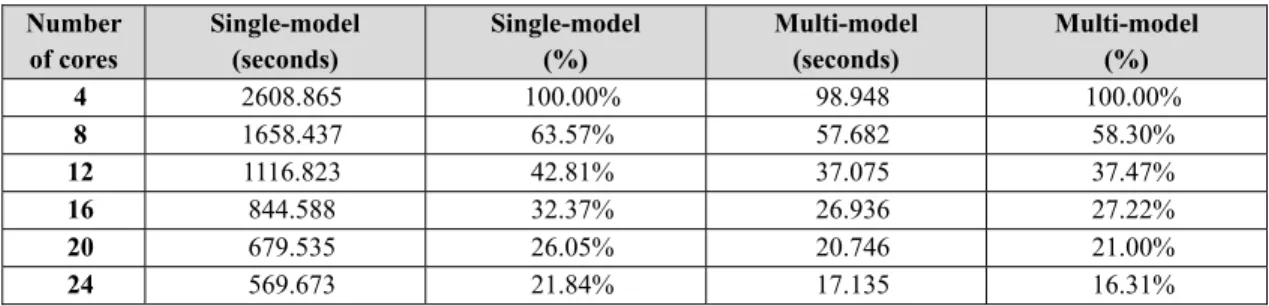
We use different number of cores to execute single-model and multi-model training session respectively and measure the training time. The result is shown in Table 1.

Table 1 Training Time Number of cores Single-model (seconds) Single-model (%) Multi-model (seconds) Multi-model (%) 4 2608.865 100.00% 98.948 100.00% 8 1658.437 63.57% 57.682 58.30% 12 1116.823 42.81% 37.075 37.47% 16 844.588 32.37% 26.936 27.22% 20 679.535 26.05% 20.746 21.00% 24 569.673 21.84% 17.135 16.31%

It is surprising that the single-model session by 4 cores takes about 43.5 minutes (2608.865 seconds), while the multi-model session by 4 cores take only 1.6 minutes (98.948 seconds). When we dig deeper into the training process, we finds out that single-model sessions takes more than 1,800 epochs to converge, while each MLP in the multi-model session takes about 250 to 500 epochs to converge. If we consider the input data for multi- model session, the training subset of each model is smaller in size and more balanced in terms of signal-zero patterns and signal-one patterns (i.e. less bias). It make sense that such characteristics results in faster convergence.

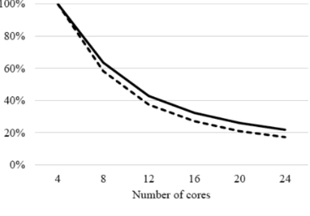
Furthermore, the percentage columns in Table 1 can be illustrated by Figure 5. The percentage is calculated based on the training time using 4 cores. In other words, the training time using 4 cores is defined as 100%, and the rest cell are derived from the training time using n cores dividing by the training time using 4 cores. The same applies to both the single-model session and the multi-model session.

It shows in Figure 5 that the trend is steeper for the percentages of multi-model session. It means the overhead of distributed computing is less for the multi-model session. It makes sense that the multi-model session has a low overhead because each MLP model is trained independently.

There is no communication needed during the training process. On the other hand, the communication during the training process is intensive in the single-model session because the distributed MLP on the master node exchanges weights with MLP clones on worker nodes frequently.

Figure 5 Training Time in Percentage

In conclusion, the multi-model training session is far more efficient than the single- model training session. In practice, it the single-model session would need a dedicated cluster since it requires intensive network communication and longer CPU time. On the other hand, the multi-model session should be deployed along with other systems of services because it is relatively lightweight in terms of network communication and CPU consumption.

Simulation

Experiment Method

In our simulation environment, an active MLP strategy receives real-time TAIs as the input vector and compute trading signals as the output. We registered some MLP strategies and perform simulated trading for simulation purpose. This experiment can also be considered as cross-validation.

Input data: As illustrated by Figure 2, there are two types of training input (a single training set and a collection of training subsets) from the preprocessing stage and each is processed by a dedicated type of training session, i.e., variant of the distributed algorithm. Furthermore, there three options for the sampling (grouping) of signal-zero parts of training subsets, as explained below.

1. Random without replacement.

3. Clustering: Signal-zero parts have high intra-group similarity and low inter- group similarity. In the following simulation we compare signal-model strategies and multi-model strategies with different grouping techniques. In addition, the period of the training set and the trading simulation is both one trading day.

I

1. Firing threshold: The output value of an MLP is a real number between zero and one, but we require the output signal to be either zero or one. If the output value is greater or equal than the firing threshold, the signal is fired as one, otherwise as zero.

2. Voting threshold: For a multi-model strategy, the final output signal is determined through voting. If the number of models firing signals of one exceeds a certain percentage of all models, the final output signal would be one, otherwise being zero. The percentage is defined as the voting threshold. In other words, the voting threshold is the confidence level required for supporting a signal-one decision.

Dependent Variables: The simulation result is analyzed with receiver operating characteristic (ROC). We have selected three most relevant measures as the dependent variables, as explained below.

1. True positive (TP): A positive is a signal of one and therefore a true positive is when a correctly predicted signal of one. In other words, for a buying put strategy, a true positive is a correct prediction of price rising (in a certain period in the future, e.g. in 10 seconds).

2. False positive (FP): On the other hand, a false positive is an incorrect prediction of price rising which represents a trading loss.

3. Positive predictive value (PPV): The positive predictive value (also called precision) is the post-test probability of an output positive being a true positive. It is the ratio of the number of true positives to the number of output positives (i.e., the number of true positives plus the number of false positives). In practice, the value should be higher than 0.5; otherwise there would be loss. The equation is as below where P’ stands for outcome positive.

PPV = TP/P′ = TP/ (TP + FP)

A valid strategy requires PPV to be higher than 0.5, yet a good strategy needs TP and PPV as higher as possible. However, it does guaranty maximized TP and PPV by minimizing the error function, which is why we need to adjust other parameters for better result.

Testing for Firing Threshold

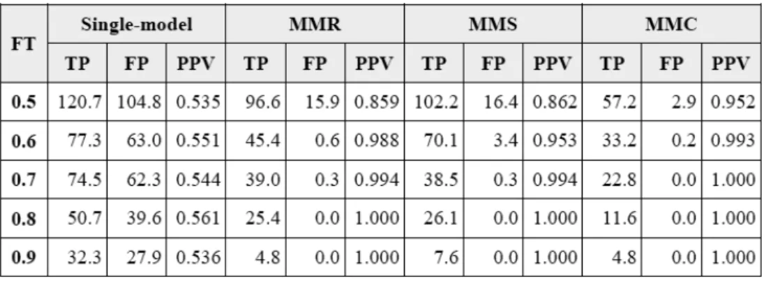
The first test takes the firing threshold (FT) as the independent variable. The value of firing threshold defaults to 0.5 (i.e., rounding of the output value) but can be increased. The simulation result of strategies with different levels of FT is shown in Table 2 (Notes. FT = firing threshold, MMR = multi-model with random sampling, MMS = multi-model with stratification, MMC = multi-model with clustering).

When FT increases, all multi-model strategies shows increasing PPV. As we would normally expect, higher firing threshold yields more conservative result. A conservative trading strategy makes fewer orders but the probability for each order to actually make a profit is higher. However single-model strategies does not show the same kind of trend.

In addition, when comparing the four type of training, the single-model session perform worse. While producing more outcome positives (TP + FP) than multi-model strategies, single-model strategies produce PPVs barely over 0.5. MMR and MMS strategies produce similar results in terms of PPV but MMS strategies produce more positives. MMC strategies produce the highest PPVs but the least positives.

Testing for Voting Threshold

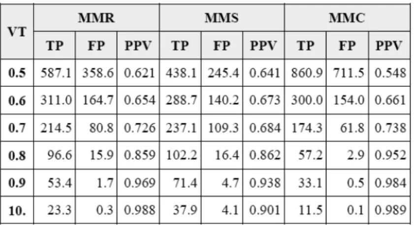
The second test takes the voting threshold (VT) as the independent variable. The value of firing threshold defaults to 0.8 but can be adjust between 0.5 and 1.0. The simulation result of strategies with different levels of VT is shown in Table 3. Only multi-model strategies are tested since there is no need for voting in a single-model strategies. In addition, the firing threshold in this test is set to the default value of 0.5.

Table 3 Result of Voting Threshold Test

When VT increases, all multi-model strategies show increasing PPV. As we would normally expect, higher voting threshold yields more conservative result. Considering the number of outcome positives and PPV, MMR strategies performs better at low levels of VT (0.5 and 0.6) but has few advantage over MMS strategies at VTs above 0.7. MMS strategies produce the least positives at low VTs but the most positives at VTs above 0.7. While MMS does not always produce the highest PPV but when taking outcome positives into account, it seems to be the most stable. MMC strategies produce the most positives at VT of 0.5 but the PPV is only 0.548. When the VT increases, the outcome positives produced by MMC decreases dramatically. Comparing all strategies, the default value of VT = 0.8 could be too conservative. It is acceptable to use 0.7 or even lower level of VT.

Considering the results of all experiments, single-model strategies clearly has no advantage over multi-model strategies and require far more time and computing resources. It seems quite reasonable to abandon single-model MLP strategies. On the other hand, MMS seems to be the most recommended in all three types of multi-model strategies.

Conclusion

Among several mining algorithms adopted in the system, this research focuses on the artificial neural network. Following the guide by Kaastra and Boyd (1996), we propose a distributed framework of ANN. The framework is designed with various options to the construction and training of a neural network. For performance, scalability and fault tolerance, we implement the framework using Scala and Apache Spark while retaining the flexibility for a different based cluster.

Although the motivation of developing a distributed framework is to accelerate the single-model training session, the results of experiments show that single-model strategies has no advantage over multi-model strategies. However, the framework also works well with multi-model training sessions, and multi-model strategies produce excellent prediction result in the trading simulation.

There is no optimal solution in neural network modeling. One can only find a better approximation through repeated trial-and-error processes. Hence the framework provides flexibility, allowing the user to experiment on various MLPs with different configurations. In this research, only a few combinations of parameters are used in the experiment, yet the result proves MLP’s exceptional ability in predicting financial time series.

Acknowledgements

This research is partially supported by the “The Cloud for the Strategy Trading” project with Chunghwa Telecom.

References

Andonie, R., Chronopoulos, A., Grosu, D., & Galmeanu, H. (1998). Distributed backpropagation neural

networks on a PVM heterogeneous system. Paper presented at the Parallel and Distributed Computing

and Systems Conference (PDCS'98).

Chen, M., Mao, S., Zhang, Y., & Leung, V. C. (2014). Big data: Related technologies, challenges and future

prospects: Springer.

Dahl, G., McAvinney, A., & Newhall, T. (2008). Parallelizing neural network training for cluster systems. Paper presented at the Proceedings of the IASTED International Conference on Parallel and Distributed Computing and Networks.

Feng, A. (2013). Spark and Hadoop at Yahoo: Brought to you by YARN. Retrieved from http://ampcamp. berkeley.edu/wp-content/uploads/2013/07/andy-feng-ampcamp-3-presentation-Spark_on_YARN.pdf Ganeshamoorthy, K., & Ranasinghe, D. (2008). On the performance of parallel neural network implementations

on distributed memory architectures. Paper presented at the Cluster Computing and the Grid, 2008.

CCGRID'08. 8th IEEE International Symposium.

Gu, R., Shen, F., & Huang, Y. (2013). A parallel computing platform for training large scale neural networks. Paper presented at the Big Data, 2013 IEEE International Conference.

Ho, S. H. (2014). Distributed Framework of Artificial Neural Network for Planning High-Frequency Trading

Strategies. (Master, National Chengchi University). Retrieved from http://nccur.lib.nccu.edu.tw/handle/

140.119/69191

Jones, R. D., Lee, Y., Barnes, C., Flake, G., Lee, K., Lewis, P., & Qian, S. (1990). Function approximation

and time series prediction with neural networks. Paper presented at the Neural Networks, 1990., 1990

Kaastra, I., & Boyd, M. (1996). Designing a neural network for forecasting financial and economic time series.

Neurocomputing, 10(3), 215-236.

Kimoto, T., Asakawa, K., Yoda, M., & Takeoka, M. (1990). Stock market prediction system with modular

neural networks. Paper presented at the Neural Networks, 1990., 1990 IJCNN International Joint

Conference on.

Liu, Z., Li, H., & Miao, G. (2010). MapReduce-based backpropagation neural network over large scale mobile

data. Paper presented at the Natural Computation (ICNC), 2010 Sixth International Conference on.

Padgavankar, M., & Gupta, S. (2014). Big Data Storage and Challenges. International Journal of Computer

Science & Information Technologies, 5(2).

Pethick, M., Liddle, M., Werstein, P., & Huang, Z. (2003). Parallelization of a backpropagation neural

network on a cluster computer. Paper presented at the International conference on parallel and distributed

computing and systems (PDCS 2003).

Sudhakar, V., & Murthy, C. S. R. (1998). Efficient mapping of backpropagation algorithm onto a network of workstations. Systems, Man, and Cybernetics, Part B: Cybernetics, IEEE Transactions on, 28(6), 841-848.

Suresh, S., Omkar, S., & Mani, V. (2005). Parallel implementation of back-propagation algorithm in networks of workstations. Parallel and Distributed Systems, IEEE Transactions on, 16(1), 24-34.

White, H. (1988). Economic prediction using neural networks: the case of IBM daily stock returns. Paper presented at the Neural Networks, 1988., IEEE International Conference.

Xin, R. S., Rosen, J., Zaharia, M., Franklin, M. J., Shenker, S., & Stoica, I. (2013). Shark: SQL and rich

analytics at scale. Paper presented at the Proceedings of the 2013 ACM SIGMOD International

Conference on Management of data.

Yoon, H., Nang, J. H., & Maeng, S. (1990). A distributed backpropagation algorithm of neural networks on

distributed-memory multiprocessors. Paper presented at the Proceedings of the 1990 Frontiers of Massively

Parallel Computation, (pp. 358-363).

Zaharia, M., Chowdhury, M., Das, T., Dave, A., Ma, J., McCauley, M., . . . Stoica, I. (2012). Resilient

distributed datasets: a fault-tolerant abstraction for in-memory cluster computing. Paper presented at the

處理巨量資料分析之分散式類神經網路

框架設計－以金融時間序列資料為例

【摘要】

斂，進行預測時在0.7 投票閥值（voting threshold）設定下採用分層多重模型（multi-model with stratification）可獲得最多的真陽性結果且準確率達 70%左右。

在我們所建構的系統裡，類神經網路是用在資料採礦階段來發掘金融時間序列資料之模式。 我們將訓練類神經網路的框架建置在分散式運算平台上，該平台我們採用具高效能記憶體內運算 （in-memory computing）的 Apache Spark 來建造底層基礎的運算叢集環境。我們評估了一些特 別適用於預測金融時間序列資料的分散式後向傳導演算法，加以調整並整合進我們所設計的框 架。同時，我們也提供了許多細部的選項，讓使用者在進行類神經網路建模時能有很高的客製化 彈性。