國
立
交
通
大
學
資訊工程學系
碩
士
論
文
行動計算環境中有效率之協同快取置換機制
An Efficient Collaborative Cache Replacement in Mobile
Computing Environments
研 究 生:張修維
指導教授:彭文志 教授
行動計算環境中有效率之協同快取置換機制
An Efficient Collaborative Cache Replacement in Mobile
Computing Environments
研 究 生:張修維 Student:Hsio-Wei Chang
指導教授:彭文志 Advisor:Wen-Chih Peng
國 立 交 通 大 學
資 訊 工 程 學 系
碩 士 論 文
A ThesisSubmitted to Department of Computer Science National Chiao Tung University
College of Electrical Engineering and Computer Science in partial Fulfillment of the Requirements
for the Degree of Master
in
Computer Science and Information Engineering
October 2005
Hsinchu, Taiwan, Republic of China
摘
要
由於近年來行動傳輸技術的快速發展,人們可以經由無線網路隨時隨地存取 各式各樣的服務。值得注意的是,由於手持裝置的快取空間和傳輸頻寬是有限的。 若我們能有一個適當的快取置換機制,則等待服務的時間就能減少。在這篇論文 中,我們專注於在無線行動環境上的快取問題。藉由整合客戶端和基地台端的快 取空間,我們提出了一個有效率的協同快取置換演算法。在我們提出的演算法裡, 我們推導出一個包含了數個重要因子的得益方程式,並且同時考量了區域性服務 以及非區域性服務。藉由此方程式,我們可以評定出每一個儲存在快取空間內資 料的得益值,以利將來的快取置換。除此之外,我們更發展了一個介於客戶端和 基地台端之間的協同機制。實驗結果顯示出我們提出的方法是非常有效率且優於 傳統的快取置換機制。 關鍵字:行動計算,區域性服務,快取置換
Abstract
Owing to the recent great advances in mobile communication technology, more and more information services are available via wireless networks. As such, users are able to access a variety of services from anywhere at anytime. Note that with proper caching mechanisms, the response time of services is reduced. Due to the limited size of local cache and transmission bandwidth of handheld devices, in this paper, we address the cache problem of mobile computing environments. By integrating cache usages in both mobile devices and base stations, we propose an efficient collaborative cache replacement (referred to as CCR) algorithm. In our proposed algorithm, we derive a profit function which includes several important factors of both location dependent service and location independent service. In light of the profit function devised, we can evaluate the profit of each cached service object for cache replacement. In addition to deriving a profit function, we further develop a collaboration mechanism between mobile devices and base stations. The experiment results show that the proposed CCR is very effective and outperforms the conventional cache replacement policies.
誌
謝
這篇論文的完成我必須感謝許多人,首先要感謝我的指導教授彭文志老師。 他不但在這兩年的碩士生涯中,教導我許多專業的知識,尤其是在資料探勘以及 行動計算方面。除此之外,他更教導了我做事情和做學問的態度,不但可應用在 求學方面,往後出了社會也是相當受用。感謝彭老師兩年來的耐心教導和包容, 我才能順利完成論文並且拿到學位。 感謝我的口試委員沈錳坤老師以及黃俊龍老師,謝謝老師在很急迫的時間內 看完我不甚嚴謹的論文,並且給了我許多寶貴的意見和忠告。再來要謝謝語文所 的郭志華老師,在這兩年裡提供我製作科技英文網頁的機會,讓我能夠賺取生活 費,並且時常關心我並且給我鼓勵。還有要謝謝實驗室的伙伴們,不論在修課或 是做研究時能一起互相討論,平日也都會互相為彼此加油打氣,共同度過層層難 關。 最後我要謝謝我的家人們,因為有你們在背後的全力支持和鼓勵,我才有辦 法如期完成我的學業。僅以這篇論文獻給所有曾經關心過我的人們。
Contents
1 Introduction 4
2 Preliminaries 11
2.1 Attributes of Service Object . . . 11
2.2 Mobile Service System Architecture . . . 12
3 Collaborative Cache Replacement Algorithm 13 3.1 Deriving Factors of Profit function . . . 13
3.2 Collaborative Cache Replacement Algorithm . . . 18
3.2.1 Cache Maintenance of CCR . . . 19
3.2.2 Actions of Base Station . . . 22
3.2.3 Actions of Client . . . 23
4 Performance Analysis 24 4.1 Simulation Model . . . 24
4.2 Experimental Results . . . 25
4.2.1 Impact of Client’s Maximum Step . . . 27
4.2.2 Impact of Client Cache Capacity . . . 30
4.2.3 Impact of Maximum Object Size . . . 30
4.2.4 Impact of LDSProb . . . 34
List of Figures
1 Mobile computing environment model . . . 5
2 Example of handling LDS . . . 8
3 Problem in handling LDS . . . 9
4 Architecture of mobile computing environment . . . 12
5 Example of service range . . . 15
6 Interaction between clients and base stations . . . 19
7 Two kinds of caches . . . 20
8 The data structure of pyramidal selection scheme . . . 22
9 Client hit ratio under various of the client’s maximum moving step . . . 28
10 Base station hit ratio under various of the client’s maximum moving step . . . 28
11 Client query cost under various of the client’s maximum moving step . . . 29
12 Base station query cost under various of the client’s maximum moving step . . 29
13 Client hit ratio under various cache capacity . . . 30
14 Base station hit ratio under various cache capacity . . . 31
15 Client query cost under various cache capacity . . . 31
16 Base station query cost under various cache capacity . . . 31
17 Client hit raio under various maximum sizes of objects . . . 32
18 Base station hit raio under various maximum sizes of objects . . . 32
19 Client query cost under various maximum sizes of objects . . . 33
20 Base station query cost under various maximum sizes of objects . . . 33
21 Client hit ratio under various of LDSProb . . . 34
22 Base station hit ratio under various of LDSProb . . . 35
23 Client query cost under various of LDSProb . . . 35
List of Tables
1 Description of symbols . . . 14
2 Distance and level sequence of Si . . . 17
3 Level count . . . 17
4 Parameters of simulation model . . . 26
1
Introduction
Owing to the recent great advances in mobile communication technology, more and more information services which provided via wireless network are available. We can anticipate that in the near future world, people can use their handheld devices to access a variety of services everywhere. For example, a driver can use a portable computer equipped with GPS to get information like traffic report, weather report, nearest gas station and restaurant. Further more, the computer can plan a traffic route which can guide the driver to avoid heavy traffic, to fuel up, than to have lunch in the nearest seafood restaurant. Also, the passenger on this car can receive and watch video or play games supplied by the broadcasting station.
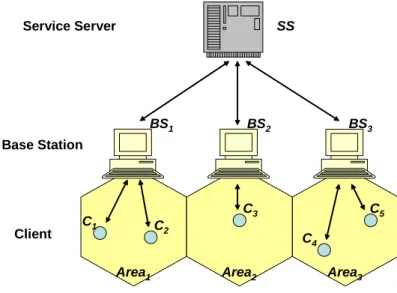
To achieve above scenarios, we must construct a suitable framework. The mobile com-puting environment model is shown in Figure 1, where the network consists of three parts: service server (SS), base station (BS), and client (C). Service servers are constructed by service providers, which store and maintain all kinds of services. Base stations are the intermediates between service servers and mobile clients. They provide wireless access points and handle the requests of mobile clients in their managing areas via wireless channel and then obtain the required data from service servers via fixed network. Mobile clients can move among service areas haphazardly, and they can discover and access services what they want.
To improve the system efficiency, mobile devices often store certain hot data in the local cache for future using, but the size of local cache in the handheld devices is limited. When an object comes and the local cache is full, we must pick some cached data and remove them from the cache to make enough space for the new coming data. In mobile service networks, the storage and computing capability of portable devices are relatively small compared to desktop computers. Due to this constraint, we must take good care of the cache storage to gain more efficiency, so the cache replacement problem is significant to the system performance. Different from traditional cache replacement algorithms in operating system and database
Service Server SS
Base Station
BS1 BS2 BS3
Area1 Area2 Area3
Client C1 C 2 C3 C4 C5
Figure 1: Mobile computing environment model
system, several characteristics are found in mobile computing environment: (1) The size of cached data may be different. In the traditional operating system, the units of the data objects are the same, which are called page or block. However, in mobile service networks, the size of data can vary from bytes to megabytes. (2) There are a huge number of mobile users in the mobile environment. Compared to the operating system or the database system, this environment is more complicate and highly dynamic. With good caching methods, we can decrease the transmission overhead, and have shorter response time. (3) There are two categories of service: Location Dependent Service (LDS) and Location Independent Service (LIS). The information of LDS is various in different areas. For example, the traffic report is distinct according to different location. The access probability of LDS will be different due to the accessed location. For example, if restaurant R is located in area A, the access probability of restaurant R becomes smaller if the client leaves the area A. The more distance apart from area A, the less access rate of restaurant R is. Oppositely, the content and access rate of LDS are invariable anywhere, such as news report. Location dependent services have their own valid scopes, which indicate the valid areas of the service. For example, the traffic report of area 1 is not suitable for service area 2. Above factors make the design of cache replacement algorithm a challenge. In mobile computing environments, users can get the desired data
instantly if the data are cached in the user’s handheld device. If not, user can use the device to send request messages to the base station, and the base station either sends the requested data back if it has cached the data or it can acquire the data from service servers. When an user requests a service, he may expect the response time of the service is short. Obviously, if we get higher cache hit rate in both client and base station caches, the response time will be reduced.
In this paper, our goal is to devise an efficient cache replacement algorithm for the mobile computing environments. We briefly survey and categorize some traditional cache replacement schemes here [2].
1. Key-based replacement method : The key-based replacement method is to sort data based on a primary key, break ties based on a secondary key, and so on. For example, the well-know Least Recently Used (LRU) algorithm is to treat access time as the first key. If there is no sufficient cache space for the new coming data, the system will prune off the data which are least recently used. LRUMIN is the method which is biased in favor of smaller sized data so as to minimize the number of data replaced. If the size of an incoming object is S and there is not enough cache space for it. We will check whether there is any object in the cache which has size at least S, and we remove the least recently used such objects from the cache. If there is no object whose sizes at least S, we start removing data in LRU order of sizes at least 1/2 S, then the data with sizes at least 1/4 S, and so on. In First In First Out (FIFO) algorithm, the key is the timestamp when the data entry the cache. We will pick the data which came into the cache earliest. In the SIZE policy, the data are removed according to data sizes. The object with the largest size is removed first.
replacement method is to employ a general profit value function to evaluate the importance of each data. The profit function is combined with certain attributes of data, such as size, access count, time since last access, entry time, transfer cost. The data with smaller profit values will first be removed. In [2], the au-thors derived the Pyramidal Selection Scheme for cache replacement in Web proxy which considers the access cost, expiration time and size of data. In [8], the au-thors proposed a gain-based cache replacement policy, Min-SAUD for the wireless data dissemination system. The policy takes access rate, size, update frequency, cache validation delay into consideration and is suitable for devices with different transmission bandwidths.
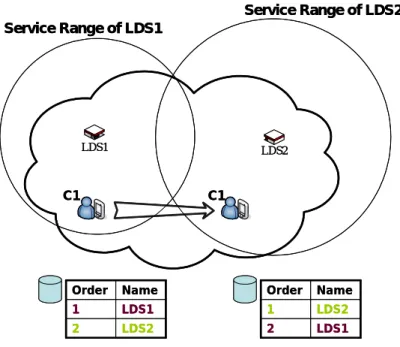
In mobile computing environments, due to the dynamic properties of the client and the characteristic of location dependent services, prior works are not totally applied on this envi-ronment. In client’s perspective, the importance of cached data is changed with the client’s location. For example, in Figure 2, LDS1 is a gas station located in area A1, LDS2 is a gas station located in area A2. When client C1 is leaving from area A1 to area A2, the importance and the access possibility of LDS1 become smaller than those of LDS2. Due to the dynamic properties of clients and the different service ranges of LDS, we must devise a method to handle this situation. For the same reason, the base station would like to store services which are near to it’s responsible location. Moreover, consider the overall cache usage in mobile computing system, where base stations may tend to store data accessed by most clients. The popular services usually have higher access possibility for coming clients than other services. If a new coming client requests the popular service cached in the base station, the base station can return it immediately without obtaining the service from the service server. On the contrary, in the client’s perspective, it would like to store services which are requested most by itself. The other challenge in mobile computing environments is that we must handle the cache replacement simultaneously of two kind of services, LDS and LIS. If
LDS1 LDS2 Name Order LDS2 2 LDS1 1 Name Order LDS1 2 LDS2 1 C1 C1 Service Range of LDS1 Service Range of LDS2 LDS1 LDS2 Name Order LDS2 2 LDS1 1 Name Order LDS1 2 LDS2 1 C1 C1 Service Range of LDS1 Service Range of LDS2
Figure 2: Example of handling LDS
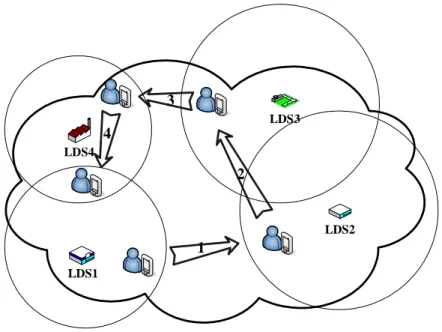
we don’t take the characteristics of LDS into consideration and just use the traditional cache replacement algorithm, some problems may occur. In Figure 3, if the cache size of the client is 3. When he is moving from LDS1 to LDS3 via LDS2, the cache is full. When he moves to LDS4 and accesses it, with LRU algorithm, the client will remove LDS1 from the cache and puts LDS4 into the cache. When he moves to LDS1 and sends a request of LDS1 in the next step, a cache miss will occur. In this situation, we must discard LDS2 rather than LDS1 since LDS2 is far away from the client.
In this paper, we propose Collaborative Cache Replacement (referred to as CCR) algorithm which takes both location dependent and independent service into consideration. Furthermore, by the collaboration between clients and base stations, we can make the caching usage of entire environment more efficient. In CCR, we consider a variety of important factors such as data size, life time, access rate, and three novel factors: popular factor, location factor, and scope factor. Popular factor represents the popularity in one service area of data. Data objects with higher popular factors mean that these data are very hot. The later coming user may be interested in these data objects. Location factor and scope factor are used for location
1 2 3 4 LDS1 LDS2 LDS3 LDS4
Figure 3: Problem in handling LDS
dependent services. Assume that each location dependent service has its own service area. If the location of accessed service is near to the location where the service resides, then it has higher location factor. Besides, scope factor represents the service range. A service with a broader service range has higher scope factor. For example, the scope factor of a gas station is larger than that of a public telephone. Otherwise, the service ranges of some services may change with time or specific events. For example, the service range of an ice shop is larger in summer than in winter, the service range of a hospital may increase when the influenza occurs. We must devise a dynamic scope factor to accommodate this situation. In addition to deriving the profit function, we also construct a collaboration mechanism between clients and base stations. Through this mechanism, a base station can adjust the caching priority according to the caching situation of clients in its service area. Base stations can know which data are popular and keep them in the cache. Thus, we can have the best overall performance. To the best of our knowledge, prior works don’t consider cache replacement by integrating both client and base station.
put much efforts on Web proxy caching [1][2][13]. We briefly introduce some traditional meth-ods for cache replacement in Web proxy servers. In [1], the authors observed that the doc-uments with small size are accessed frequently. The LRU-MIN cache replacement algorithm was proposed to handle the small document retrieval. It first tests whether there are any documents equal or larger in size than incoming document; if there is, the algorithm chooses one of them by LRU. A function-based cache replacement PSS policy was proposed in [2]. The author employed a potentially general function of different factors such as size, time since last access, entry time and so on to decide which object is going to be replaced. Recently, Chang and Chen proposed caching replacement for transcoding proxy [4]. Transcoding proxy is used for transformation between multimedia objects in different versions and resolutions. A weighted transcoding graph was devised to manage multiple versions of different objects cached in transcoding proxy. In mobile environments, there are a lot of researches focused on cache consistency. The authors in [3] presented three invalidation report (IR) based schemes for cache consistency. The server will send invalidation reports to clients to inform which object is invalid and replaced. Many of later proposed cache invalidation schemes are variants of the above IR schemes [5][7][9][17], and these researches are devoted to designing efficient al-gorithms to reduce IR overhead and to improve uplink cost. All of these invalidation schemes result in cache invalidation delay for confirming the data consistency before the object is used. More recently, much work puts emphasis on location dependent services [6][12][14][15]. In [15], the author studied the cache consistency issue for location-dependent information in the context of mobile environments. For location-dependent updates, three invalidation schemes called BVC, GBVC, and ISI are proposed. Other work try to cache some frequently queried data in client side [6][12]. The authors in [12] found that the location dependent query is more likely to exhibit a semantic locality in terms of locations rather than spacial locality. In [6], the authors proposed a proactive caching model for spacial queries. The proactive caching captures the semantics of queries by caching the index responsible for querying. The
authors in [14] presented dynamic location dependent data management to replicate the data of the most frequently accessed neighborhood cells at the local server. Some researches deal with the caching strategy in ad hoc networks [16][11].
The rest of this paper is organized as follows. In Section 2, we describe the system architec-ture of CCR and some attributes of data objects. In Section 3, we derive the profit function and the CCR algorithm. The metric measurement and simulation results are presented in Section 4. This paper concludes with Section 5.
2
Preliminaries
To facilitate the presentation of this paper, we describe the attributes of service object in Section 2.1. In Section 2.2, we briefly introduce the architecture of the mobile service system.
2.1
Attributes of Service Object
Following we describe the attributes that can represent the statuses of a service objects for cache replacement.
(1) Size : The size is an important attribute for cache replacement policy. Most cache replacement algorithm tends to prune off the data with large sizes to make more sufficient space for later data. (2) Expire time : The attribute to indicate the life time of an object. We can discard an object with less life time. (3) Access Count : It is dynamic statistic in both base station and client for traditional counting-based cache replacement algorithm. The objects with higher access frequency indicate that the objects are hot. (4) Last access time : It is the timestamp which is recorded when the objects are accessed the last time. This information is used for traditional LRU algorithm. (5) Residing location : The information which is used for location dependent service. We assume a geometric location model in this paper, and the location is specified as a two-dimensional coordinate. Services can identify
Central Database LIS Manager LDS Manager Scope Factor Handler Service Server Central Database Central Database LIS Manager LIS Manager LDS Manager Scope Factor Handler LDS Manager Scope Factor Handler Service Server Local Cache Local Cache LIS Manager LIS Manager Base Station LDS Manager GPS LDS Manager GPS Client Manager Client Manager Cache Cache LIS Manager LIS Manager Client
Inform location of data,
Request of data Return of data
Register, Request of data Return of data LDS Manager GPS LDS Manager GPS
Figure 4: Architecture of mobile computing environment
their location by their service providers using GPS. (6) Furthest access location : It is the location where the object is accessed furthest. The information is used for location dependent service, and it is kept in service server. We can use this information to represent the service range. 8) Access client count : The number of access client which access the object in this area. The record is kept in the base station. If the number is large, we can say that this object is popular.
2.2
Mobile Service System Architecture
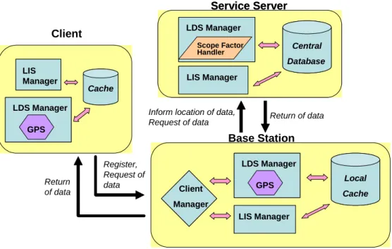
The mobile computing environment we describe here must accommodate two conditions. First, the system must serve both location dependent service (LDS) and location independent service (LIS). Second, it must be suitable for the mobile environment in the present and the future. As Figure 4, the system architecture is composed of three components.
(1) Service Server : The service servers store all kinds of information and services. There are a variety of service providers such as map service, traffic report service, news service. When a service provider wants to publish its services into the environments, it must register
its services to the service server including name, size, expire time and the residing location. The service server is connected with the base station via fixed wired network. The main task of the service server is to receive requests from base stations and to send requested service objects back. Service servers have two kinds of service managers : LDS manager and LIS manager. LDS manager has a scope factor handler to handle the scope factors of all data. (2) Base Station : As we mentioned in Figure 1, all base stations have their own service areas. The base stations keep tracking all clients who are active in their own service areas. Similar to service servers, the base station must take responsibility to serve the clients in their service areas. Furthermore, they gather some statistics of services accessed by the clients in their service areas such as last accessed time and accessed frequency. The base station has a local cache to store some specific data for future using. (3) Clients : The clients vary from laptop computers to smartphones. People use them to send requests to base stations through wireless communication and get desired services. Also, all clients have small cache storage to keep some useful data and gather statistic of data. Clients can move from a service area to another.
3
Collaborative Cache Replacement Algorithm
In Section 3.1, several important factors are presented for the derivation of the profit function. In Section 3.2, according to profit functions, we develop the collaborative cache replacement algorithm.
3.1
Deriving Factors of Profit function
In traditional counting-based cache replacement algorithms, the access count is an important information for cached objects. Usually, object with high access count represents that the object is very hot to users. Obviously, systems which cache such kind of objects will gain
Symol Description
ACij Access count of service Si in client Cj or in base station Bj
T ACj Total access count of all cached services in client C
j or base station Bj
AFij Access factor of service Si in client Cj or base station Bj
Tisj Timestamp of service Si enter client Cj or base station Bj
Tie Expire time of service Si
LTij Life time of service Si
T Fij Time factor of service Si in client Cj or base station Bj
ADi Access distance of serice Si
LFi Location factor of service Si in client Cj or base station Bj
Di Distance sequence of serice Si
Li Level sequence of serice Si
SFi Scope factor of service Si
SCij Total count of clients which cache Si in Bj
T Cj Total count of clients in Bj
P Fij Popular factor of Si in Bj
Table 1: Description of symbols
more cache hit rates. Here, we want to normalize this information to one of the terms in the profit function.
The access count, denoted by ACij presents the access count of service Si in client Cj or
in base station Bj. Both clients and base stations keep these statistics of all cached services
in their cache. Total access count, denoted by T ACj, presents the total access count of all
cached services in Cj or Bj, and T ACj =
n
P
i=1
ACij. We have the access factor AFij of Si in Cj
or Bj as follows :
AFij = 1 +
ACij
T ACj
Services in mobile computing environments often be assigned expiration times. If a service is going to expire, it probably need to be discarded soon. This kind of service should be
a good candidate for replacement. Suppose Si is in the cache of Cj or Bj at time Tisj, and
the expire time of service Si is Tie. We define the life time of service Si, denoted by LTij,
such that LTij = Tie− T
j
is. Then we define the active time of service i, denoted by ATi, and
LDS1 LDS2 d2 d1 d3 d4 C1
Figure 5: Example of service range
T Fij = ATi
LTij
Location factor is applied to the location dependent service. Since each LDS has its own service area, the access possibility of a LDS should be different according to the location, where it is requested. Employing this feature into the profit function will make the cache replacement
algorithm more accurate. For clients, we define the access distance of Si, denoted by ADi,
which represents the distance between the access location of Si and Si residing location. For
base stations, ADi represents the distance between the base station’s location and Si residing
location. We define the location factor of Si, denoted by LFi, as follows :
LFi = 1 + 1 d, d = ⎧ ⎪ ⎪ ⎪ ⎪ ⎪ ⎪ ⎨ ⎪ ⎪ ⎪ ⎪ ⎪ ⎪ ⎩
1, if ADi is smaller than 1
ADi
∞, if Si is LIS
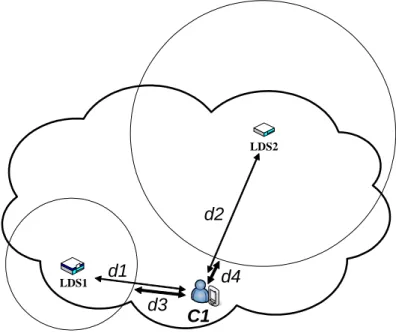
Each LDS has its own service range. For example, the service range of a public telephone may be ten or more meters, but the service range of a gas station may be several kilometers.
In Figure 5, although the distance d1 between client C1 and LDS1 is smaller than the
distance d2 between client C1 and LDS2, but the client is more close to LDS2’s service area
than LDS1’s. Note that the client C1 has higher probability in entering LDS2’s service than
LDS1’s. We must consider this feature in the profit function to give the higher priority to the
services which have larger service ranges. As mentioned before, services may have different
service ranges due to certain reasons. Let us denote the scope factor of Si as SFi. SFi is
handled by the scope handler in the service server, and it is initially set to 1. Base stations
will periodically inform service servers the access locations of all LDSs. To derive SFi, the
service server will keep top n long distances access records of Si by all the clients, which is
called distance sequence Di.
Di ={d1, d2, ..., dn}, di is the first i long distance of access records
Then we transform the distance sequence Di to level sequence Li :
Li ={l1, l2, ..., ln}, li = 1 +
¹
di
LevelT hreshold º
LevelThreshould is a system parameter which determines the range of one level. For example, in a very wide environment, we can let the LevelThreshould be 1 km. Therefore, level
1 represents that the access distance is between 0 to 1km. Then we can get M axLevel(Li) :
M axLevel(Li) = lmax,
lmax is the maximum element of Liwhich count of lmax > , is a system threshold.
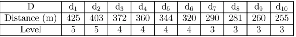
For example, if LevelT hreshold = 100m, lmax = 3, = 3, it can be verified that there are
D d1 d2 d3 d4 d5 d6 d7 d8 d9 d10
Distance (m) 425 403 372 360 344 320 290 281 260 255
Level 5 5 4 4 4 4 3 3 3 3
Table 2: Distance and level sequence of Si
Level Count
5 2
4 4
3 4
Table 3: Level count
SFi = ⎧ ⎪ ⎪ ⎨ ⎪ ⎪ ⎩ M axLevel(Li),if M axLevel(Li)≤ α α,if M axLevel(Li) > α
Where α is a system parameter which is the upper bound of service range.
For example, we give LevelT hreshold = 100m, = 3, α = 5. If the access record is as
Table 2. The result is shown in Table 3. Therefore, SF = 4.
In the base station’s perspective, data items with high access counts are not sure that they are really hot. Perhaps these data are accessed by few individual people. On the other hand, the base station should keep the popular services as much as possible. We derive popular
factor to add weights to those popular data. Considering service Si in base station Bj, we
define SCij as the total count of clients that cache Si in Bj and T Cj as the total count of
clients in Bi. Popular factor of Si in Bj, denoted by P Fij, is defined as follows :
P Fij = 1 + SC
j i
T Cj
Based on the above discussion, in the base station, we tend to keep popular object with high access frequency, long life time, small data size, high location factor, and high scope factor in the cache. So we simply multiply all factors and divide size to obtain the profit function applied to the base station, denoted by B_P rof it(i) as following :
B_P rof it(i) = AFi× T Fi× LFi× SFi× P Fi
Sizei
Otherwise, the client is moving around and just focuses on his own usage. When we derive the profit function of the client, we evict the PF from the function as follows :
C_P rof it(i) = AFi× T Fi× LFi× SFi
Sizei
3.2
Collaborative Cache Replacement Algorithm
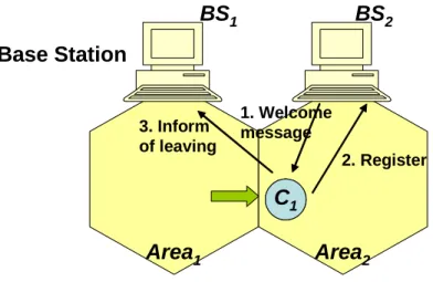
In Section 3.1, we have formulated the profit function of cache replacement. Based on the profit function, we derive the Collaborative Cache Replacement algorithm in this section. In CCR, both clients and base stations have individual cache replacement algorithms themselves. The main idea of CCR is to sort cached data according to their profit values, to keep the data with higher profit values, and then to discard those data with values lower. The main difference between clients and base stations is that the clients are active and moving, yet the base stations are passive and static. Clients may move from one base station to another, and they probably send requests of services to the base stations. The interaction between clients
and base stations is shown by Figure 6. When a client C1 enters a new service area Area2, the
base station BS2 of Area2 will detect and send a welcome message to C1. When C1 receives
the message, he knows that he is entering a new service area, and then he sends information
such as client id and cached objects’ id, and registers them to BS2. When BS2 receives these
records, it computes and updates the profit values of cached data. Afterward, C1 informs BS1
for leaving. Then BS1 removes C1 from the client list, computes and updates the profit values
Base Station BS1 BS2 Area1 Area2 C1 C1 3. Inform of leaving 2. Register 1. Welcome message
Figure 6: Interaction between clients and base stations
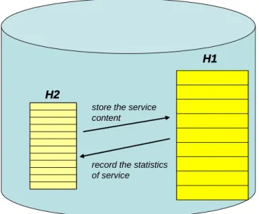
3.2.1 Cache Maintenance of CCR
In order to have a good cache replacement mechanism, we employ a small auxiliary cache H2
which maintains the statistic of some numbers of data, as shown in Figure 7. The H2 can help
us to keep a period of statistic records of the removed data. In a heavy loading environment,
employing large H2 can prevent system from removing data rapidly without gathering any
statistics on them. Therefore it can improve the accuracy of CCR. The H2 is constructed by
Heap data structure. In H2, we keep the passed statistic records of data including size, access
count, access time, expire time and residing location. The size of H2 is β ×(size of H1), β is
an adjustable system parameter. When the number of services is tremendous or the access frequency of system is very high, we could set a big value of β.
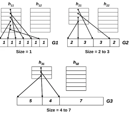
To decrease the maintaining cost of H2, we employ the Pyramidal Selection Scheme[2],
to design a cache management algorithm, named Pyramidal Replacement Algorithm (PRA). The primary idea of the PRA is to make a pyramidal classification of service objects upon
their sizes. In H1, the objects of group i have sizes ranging from 2i−1 to 2i-1. Therefore,
we will have N = dlog2(S + 1)e different groups of objects, where S is the maximum size of
service objects. In Figure 8, for each group Gi in H1, we have two heaps hi1 and hi2 in H2.
H2 H2
H1 H1
store the service content
record the statistics of service
Figure 7: Two kinds of caches
pointing the address of cached service object in Gi. The hi2 simply stores the statistics of
service objects whose size ranges are contained in Gi, but the contents are not cached in Gi.
The entries in hi1 and hi2 are sorted by profit values. In hi1, the first entry has the smallest
profit value. But in hi2, the entry with the biggest profit value will be placed in the first. It is
because that all the entries in hi2are the candidates to replace the entries in hi1. For example,
if the entry hi2(1) with the maximum profit value in hi2 is bigger than the entry hi1(1) with
the minimum profit value in hi1, we can replace hi1(1) by hi2(1) and put the content of hi2(1)
into H1. In PRA, we perform cache replacement in separate group. The algorithm form of
PRA is shown below. Algorithm PRA:
1 While (a request of S of group Gi comes in) {
2 if (S hit in hi1) {
3 Calculate and update Profit(S), then adjust hi1;
4 }
5 else if (S hit in hi2) {
6 calculate and update Profit(S), then adjust hi2;
7 if (hi2(1) == S) {
8 for(hn1 to h(i+1)1) {
9 if (Profit(S) > Profit(hx1(1))) {
10 move hx1(1) to hx2 then adjust hx2;
11 move hi2(1) to hi1 then adjust hi1;
12 }
14 for(hi1 to h11) {
15 select first n object of hx1, in order of Profit(Sn) and access time
16 which satisfies : n P i=1 Size(Sn) ≥ Size(S), n−1P i=1 Size(Sn) < Size(S) 17 if ( n P i=1
P rof it(Si) < P rof it(S)){
18 move this n object from hx1 to hx2 then adjust hx2;
19 move hi2(1) to hi1 then adjust hi1;
20 } 21 } 22 } 23 } 24 else{ 25 calculate Profit(S); 26 if (H1 is not full){ 27 insert S to Gi;
28 add S to hi2 and adjust hi2;
29 }
30 else if (H2 is not full){
31 insert S to hi2 and adjust hi2;
32 do the same procedure from line 7 to line 22
32 }
34 }
If a service object S comes and it belongs to group Gi. If S is in hi1, we just calculate and
update the profit value of S in hi1 and then adjust hi1. If S is not in hi1 but in hi2, it means
that we have the record of S in hi2. We first calculate and update the profit value of S in hi2
and then adjust hi2. If S becomes the root of hi2, it means that S has the biggest profit value
in hi2 and has the chance to replace other data cached in H1. In line 8 to line 13, we compare
the profit value of S with hx1(1), where the value range of x is from n to i + 1. If the profit
value of S is greater than hx1(1) for some x and the size of the object in Gx is larger than
S, we can move hx1(1) to hx2 and then move S to hi1 directly. If we do not find such hx1 in
the range of n to i + 1, we start to look for the replacement candidates in hi1 to h11 (line 14
to line 21). We select the first n data objects from hx1 sorted according to profit values, the
access time, and the total size of this n data is greater than that of S. If there are such n data objects, we calculate the sum of these n data objects’ profit values and then compare it with the profit value of S. If the profit value of S is bigger, the base station removes the n data
1 1 1 1 1 1 G1 1 1 1 1 1 1 G1 h11 h12 2 3 3 2 G2 2 3 3 2 G2 h21 h22 5 4 7 G3 h31 h32 5 4 7 G3 h31 hh3232 Size = 1 Size = 2 to 3 Size = 4 to 7
Figure 8: The data structure of pyramidal selection scheme
both hi1 and hi2, we calculate the profit value of S, and then insert S to hi2 and adjust hi2.
Finally we check whether S can replace the objects in H1 or not (line 32).
3.2.2 Actions of Base Station
There are three event-driven actions of base stations.
1. When the base station receives a request of Si : First, the base station will
check H1 to see if Si is there. If a cache hit occurs in the base station, the base
station will simply send Si back to the client. If Si does not exist in H1 but it has
some access records in H2, the base station will obtain Si from the service server
and then perform PAR. If Si does not appear in H1 and H2, the base station surely
must obtain Si from the service server and perform PRA. The last step is to send
Si back to client.
2. When a client enters or leaves the base station : Because the computing of the popular factor requires the number of clients in the service area, the base station
must always track the clients who are active in its service area. When a client comes, the base station will add the client’s identification to the client list and update the profit values of all data cached in the newcoming client. When a client leaves, the base station does the similar work.
3. Base stations periodically inform the service server the furthest access location of data : For the calculation of the scope factor, the base station will periodically inform the service server the furthest access locations of all location dependent data which it cached. The period is a system-defined parameter.
3.2.3 Actions of Client
Different from the base station, the client has two actions :
1. When a client requires a service Si : The cache replacement algorithm of the
client is the same as the base station’s. There are only two little differences : When the client does not get a cache hit in local cache, it will send the request of service to the base station in this service area. When the client receives the requested data, it will pass them to the application.
2. When a client is moving : When a client C1 is moving from the base station
B1 to the base station B2, the client will first receive a welcome message from B2.
C1 knows that he is entering a new service area, and he informs the previous base
station B1 for his leaving. The LF of cached LDS must be updated because the
client’s location is changed. The client recomputes the profit values of all affected
4
Performance Analysis
In this section, we will describe our simulation model and evaluate the performance of CCR. In Section 4.1, we illustrate the simulation model and events. Several system parameters are also introduced to facilitate our simulation. The experimental results of performance analyses will be presented in Section 4.2.
4.1
Simulation Model
The mobile computing environments consists of many service areas with their own base sta-tions, and the base stations can provide clients with a seamless service when they move between different service areas. To simulate the mobile computing environment, we use an 8×8 mesh topology network [10]. Each grid in the mesh network represents a service area, and there exists one base station which takes responsible for this service area. The base station will handle the requests of services. Therefore, there are 64 base stations in the simulation model. Each base station has the local cache with the size BCacheSize. The number of active clients is ClientNum, and we can adjust this parameter to represent the load of the environment.
The database contains two kinds of services, LDS and LIS. The numbers of them are LDSNum and LISNum, respectively. The size of service object is randomly distributed from MinSize to MaxSize. For each service, we assign a value named hot_level according to Zipf distribution from MIN_HOT to MAX_HOT with skewness parameter HOT_SKEW. Higher hot_level means that the service has higher probability to be accessed. We randomly assign each LDS one service area and range level. The transmission between clients and base stations is wireless communication, and the cost is BCCost. Relatively, the transmission between service servers and base stations is via fixed wired network, and the cost is named SBCost.
The clients are initially randomly distributed on the mesh network, and they can freely move from one service area to another and request services. The local cache size of the client
is CCacheRatio× BCacheSize. The CCacheRatio is a value between 0 to 1. The mobile clients are modeled with two independent actions : move and access. Each client will initially assign a value step_count, meaning that client will move step_count steps in the network. In the move action, the client can move from the current service area to the vicinity and decrease the step_count by one. The clients will terminate his actions when step_count is zero. If a client moves to the boundary of the mesh network, it will change direction or turn back rather than leave the network. After each move process, the client will execute access process. In access process, the client first decides the access count between MIN_ACCESS and MAX_ACCESS in Zipf distribution with skewness parameter ACCESS_SKEW. In each access, the client decides which kind of services he wants to access according to LDSProb which represents the probability of requesting LDS. Then the client will choose one service of the selecting service type according the hot_level. The access probability is distributed following the Zipf distribution from MAX_HOT to MIN_HOT. If the requested service does not exist in the client local cache, the client will send the access request to the base station in the service area where the client stays. Afterward, if the client does not have enough cache space to store the newcoming service object, it will perform cache replacement.
The base station handles the incoming requests by FCFS. When a base station receives an access request from a client, it first checks whether the accessed service is in the local cache. If it exists, the base station simply returns the result to the client. Otherwise, the base station should obtain the accessed service from the service server and performs cache replacement if necessary.
4.2
Experimental Results
In this section, the proposed CCR is evaluated based on the simulation model. Each set of the experimental results are obtained by the average of three runs of simulations. In the performance evaluation, the cache hit ratio is employed as the primary performance metric
Parameter Description
BCacheSize size of local cache in base station
ClientNum number of client
LDSNum number of LDS
LISNum number of LIS
MinSize minimum size of service object
MaxSize maximum size of service object
MIN_HOT minimum hot_level of service object
Max_HOT maximum hot_level of service object
HOT_SKEW skewness parameter of Zipf distribution
BCCost transmission cost from the base station to the client
SBCost transmission cost from the service server to the base station
CCacheRatio client cache size ratio to base station
LDSProb probability of accessing LDS
MIN_ACCESS minimum access count of client
Max_ACCESS maximum access count of client
ACCESS_SKEW skewness parameter of Zipf distribution
Table 4: Parameters of simulation model
because that most of the other performances can be derived from the cache hit ratio. We observe the cache hit ratios in both clients and base stations. In the client’s perspective, the cache hit ratio is defined as the total cache hit count in the local cache to the total access count. In the base station, the cache hit ratio is defined as the total cache hit count to the total request count in its charging service area. Besides, considering the sizes of service objects are various, the cache hit ratio may not reflect the actual performance. We employ query cost
to evaluate the performance. The query cost of client QCc is defined as :
QCc= n P i=1 SZi× BCCost n + m P j=1 SZj× (BCCost + SBCost) m
The first term represents the query cost of cache miss in the client’s local cache but cache
hit in the base station. SZi means the size of the service object which is hit and obtained
in the base station, n means the total count of such objects. The second term represents the
query cost of cache miss in the client’s local cache but cache hit in the service server. SZj
Parameter Setting Parameter Setting BCacheSize 2000 HOT_SKEW 1 ClientNum 150 BCCost 3 LDSNum 1000 SBCost 1 LISNum 1000 CCacheRatio 12.5 MinSize 15 LDSProb 2/3 MaxSize 100 MIN_ACCESS 1 MIN_HOT 1 Max_ACCESS 35 Max_HOT 5 ACCESS_SKEW 1
Table 5: Default parameter setting for simulation model
means the total count of such objects. Similarly, the query cost of base station QCb is defined
as : QCs= n P i=1 SZi× SBCost n
In each experiment, we compare the performance of CCR with the traditional LRU and LFU cache replacement algorithms. The default setting of the simulation model is shown in Table 5.
4.2.1 Impact of Client’s Maximum Step
In the first experiment, we observe the performance of our algorithm by varying the maximum moving step of clients. In the simulation model, the clients will access several data after moving a step. With the increase of the clients’ moving step, the access records will increase too. Both the client and the base station could gather more statistic for further cache replacement. The simulation results are shown in Figure 9, Figure 10, Figure 11, and Figure 12. As shown in Figure 9, we can see that the client hit ratio of CCR outperforms other algorithms. The average improvement of client hit ratio over the LRU and LFU is about 50%. The performance of LRU is the worst and it is not influenced by the variation of clients’ moving step. It is because that the LRU just takes the access time into consideration. The LFU performs better
0 5 10 15 20 25 5 10 15 20 25 30 35 40 45 50 Max step C lie nt h it ra tio (% ) CCR LRU LFU
Figure 9: Client hit ratio under various of the client’s maximum moving step
10 15 20 25 30 35 40 5 10 15 20 25 30 35 40 45 50 Max step B as e st at ion hi t ra tio (% ) CCR LRU LFU
Figure 10: Base station hit ratio under various of the client’s maximum moving step than LRU since that LFU can collect more statistic of access records with the increase of the client’s moving step. The same as CCR, if the clients move further, the CCR can gather more information of the access patterns and popularity of objects in the environment to do cache replacement precisely. In Figure 10, we can observe that all three algorithms perform well when the clients move further, because that all the base stations almost store the objects which are popular among clients. In Figure 11 and Figure 12, the query cost of CCR is much smaller than those of LRU and LFU since the cache hit ratio of CCR is higher.
150 155 160 165 170 175 180 185 190 195 5 10 15 20 25 30 35 40 45 50 Max step C lie nt quer y cos t CCR LRU LFU
Figure 11: Client query cost under various of the client’s maximum moving step
30 32 34 36 38 40 42 44 46 48 5 10 15 20 25 30 35 40 45 50 Max step B as e s ta tio n q ue ry c o st CCR LRU LFU
0 2 4 6 8 10 12 14 16 5 6 7 8 9 10 11 12 Cache capacity (%) C lie nt h it ra tio (% ) CCR LRU LFU
Figure 13: Client hit ratio under various cache capacity
4.2.2 Impact of Client Cache Capacity
In the second experiment, we investigate the influence of the various client cache capacities. The simulation results are shown in Figure 13, Figure 14, Figure 15, and Figure 16. Of course the hit ratio will be improved while the cache size is relative large. But as Figure 13, it shows that the CCR can use the cache storage more efficiently than LRU and LFU. When the client’s cache size is 12% to the base station, the improvements of client hit ratio over the LRU and LFU are 72% and 35% respectively. In Figure 14, the base station hit ratio gets smaller because in the same time the client hit ratio is getting larger, but the CCR still performs much better than others. Figure 15 and Figure 16 show the query costs of clients and base stations.
4.2.3 Impact of Maximum Object Size
Then we observe the performance under various maximum sizes of objects. The simulation results are shown in Figure 17, Figure 18, Figure 19, and Figure 20. If the possible maximum size of objects is large, the cache insufficiency will happen frequently. If the cache space is occupied by large size objects, the number of cached objects will be small, so that the hit ratio will be reduced too. The initial value of client cache is 250, so as Figure 17, all three algorithms
20 25 30 35 40 5 6 7 8 9 10 11 12 Cache capacity (%) B as e st at ion hi t r at io (% ) CCR LRU LFU
Figure 14: Base station hit ratio under various cache capacity
170 175 180 185 190 195 200 5 6 7 8 9 10 11 12 Cache capacity (%) C lie nt quer y cos t CCR LRU LFU
Figure 15: Client query cost under various cache capacity
32 34 36 38 40 42 44 5 6 7 8 9 10 11 12 Cache capacity (%) B as e st at ion que ry co st CCR LRU LFU
0 5 10 15 20 25 50 60 70 80 90 100 110 120 130 140 150 Max object size
C lie nt hi t r at io ( % ) CCR LRU LFU
Figure 17: Client hit raio under various maximum sizes of objects
20 22 24 26 28 30 32 34 36 50 60 70 80 90 100 110 120 130 140 150 Max object size
B as e st at ion hi t r at io (% ) CCR LRU LFU
Figure 18: Base station hit raio under various maximum sizes of objects
perform badly when the maximum size of object is approximate to 150, and it reaches 60% of client cache. But in other cases when the maximum sizes of objects are relatively small, the CCR performs much better than other algorithms. In Figure 18, as the maximum size of object gets bigger and the client cache hit ratio gets smaller, the base station hit ratio gets higher since there are more requests reach the base stations. Figure 19 and Figure 20 show that the query costs of all three algorithms increase dramatically with the growth of object size.
50 100 150 200 250 300 350 50 60 70 80 90 100 110 120 130 140 150 Max object size
C lie nt qu er y cos t CCR LRU LFU
Figure 19: Client query cost under various maximum sizes of objects
20 25 30 35 40 45 50 55 60 65 50 60 70 80 90 100 110 120 130 140 150 Max object size
B as e st at ion que ry cos t CCR LRU LFU
0 5 10 15 20 25 40 50 60 70 80 90 LDSProb (%) C lie nt h it ra tio (% ) CCR LRU LFU
Figure 21: Client hit ratio under various of LDSProb
4.2.4 Impact of LDSProb
Finally we adjust the access probability of LDS to observe the impact on all three algorithms. When LDSProb is large, the properties of LDS will be significant. So the cache replacement algorithms which take the characteristics of LDS into consideration will gain higher perfor-mance. The simulation results are shown in Figure 21, Figure 22, Figure 23, and Figure 24. In Figure 21, we can see that the CCR performs superiorly than LRU and LFU in higher LDSProb. Since the CCR considers the properties of LDS, so when the access probability of LDS is high, the performance of CCR is ascendant. The same situation happens in Figure 22, Figure 23, and Figure 24.
5
Conclusions
In this paper, we proposed the Collaborative Cache Replacement algorithm which takes both location dependent and independent service into consideration. By the collaboration between clients and base stations, we can make the caching usage of entire environment more efficient. We derived a profit function which considering several important factors of both location
0 5 10 15 20 25 30 35 40 45 50 40 50 60 70 80 90 LDSProb (%) B as e st at ion h it ra tio (% ) CCR LRU LFU
Figure 22: Base station hit ratio under various of LDSProb
100 120 140 160 180 200 220 40 50 60 70 80 90 LDSProb (%) C lie n t que ry cos t CCR LRU LFU
30 32 34 36 38 40 42 44 46 48 40 50 60 70 80 90 LDSProb (%) B as e st at ion qu er y cos t CCR LRU LFU
Figure 24: Base station query cost under various of LDSProb
dependent service and location independent service. By using the profit function, we can evaluate the profit of each cached service object for cache replacement. In addition to deriving profit function, we also construct a collaboration mechanism between clients and base stations. Through this mechanism, base stations can adjust the caching priority according to the caching situation of clients in their service area. Base stations can know which data are popular and keep them in the cache. The experiment results showed that the proposed CCR is very effective and outperforms the conventional cache replacement algorithms.
References
[1] M. Abrams, C. Standridge, G. Abdulla, S. Williams, and E. Fox. Caching proxies: Limitations and potentials. In Proceeding of the 4th International World Wide Web Conference, pages 119—133, December 1995.
[2] C. Aggarwal, J. Wolf, , and P. Yu. Caching on the World Wide Web. IEEE Transactions on Knowledge and Data Engineering, 11(1):94—107, January/February 1999.
[3] D. Barbara and T. Imielinksi. Sleepers and Workaholics: Caching Strategies for Mobile environments. In Proceeding of ACM SIGMOD, pages 1—12, May 1994.
[4] C.-Y. Chang and M.-S. Chen. Exploring Aggregate Effect with Weighted Transcoding Graphs for Efficient Cache Replacement in Transcoding Proxies. In Proceeding of the 18th International Conference on Data Engineering, February 2002.
[5] G.Cao. A Scalable Low-Latency Cache Invalidation Strategy for Mobile Environments. IEEE Transactions on Knowledge and Data Engineering, 15(5), September/October 2003.
[6] H. Hu, J. Xu, W. Wong, D. L. B. Zheng, and W.-C. Lee. Proactive Caching for Spa-tial Queries in Mobile Environments. In Proceeding of 21th IEEE Int. Conf. on Data Engineering (ICDE ’05), April 2005.
[7] Q. Hu and D.-L. Lee. Cache Algorithms Based on Adaptive Invalidation Report for Mobile Environments. Cluster Computing, 1(1):39—48, February 1998.
[8] Q. H. J. Xu, W.-C. Lee, and D. Lee. Performance Evaluation of an Optimal Cache Replacement Policy for Wireless Data Dissemination. IEEE Transactions on Knowledge and Data Engineering, 16(1), January 2004.
[9] A. Kahol, S. Khurana, S. Gupta, and P. Srimani. A Strategy to Manage Cache Consis-tency in a Distributed Mobile Wireless Envionment. IEEE Transactions on Parallel and Distributed Systems, 12(7):686—700, July 2001.
[10] Y. B. Lin. Modeling Techniques for Large Scale PCS Networks. IEEE Comm. Magazine, 35(2):102—107, Feburary 1997.
[11] B. Liu, W.-C. Lee, and D. Lee. Distributed Caching of Multi-dimensional Data in Mobile Environments. In Proceeding of IEEE Infocom 2004, March 2004.
[12] Q. Ren and M. Dunahm. Using Semantic Caching to Manage Location Dependent Data in Mobile Computing. In Proceeding of the MOBICOM Conference, pages 210—221, 2000. [13] S. Williams, M. Abrams, C. Standridge, G. Abdulla, and E. Fox. Removal Policy in Network Cahces for World Wide Web Documents. In Proceeding of ACM SIGCOMM, pages 293—304, 1996.
[14] S.-Y. Wu and K.-T. Wu. Dynamic Data Management for Location Based Services in Mobile Environments. In IDEAS2003: The 7th International Database Engineering and Application Symposium, pages 180—189, July 2003.
[15] J. Xu, X. Tang, and D. Lee. Performance Analysis of Location-Dependent Cache Inval-idation Schemes for Mobile Environments. IEEE Transactions on Knowledge and Data Engineering, 15(2), March/April 2003.
[16] L. Yin and G. Cao. Supporting Cooperative Caching in Ad Hoc Networks. In Proceeding of IEEE Infocom 2004, March 2004.
[17] J. Yuen, E. Chan, K. Lam, and H. Leung. Cache Invalidation Scheme for Mobile Com-puting Systems with Real-Time Data. ACM SIGMOD Record, 29(4):34—39, 2000.