自動眼睛偵測及眼鏡去除方法

全文

(1)國立交通大學電機與控制工程研究所. 碩士論文. 自動眼睛偵測及眼鏡去除方法 Automatic Eye Detection and Glasses Removal. 研. 究. 生：王聖文. 指導教授：張志永. 中華民國九十三年六月.

(2) 自動眼睛偵測及眼鏡去除方法 Automatic Eye Detection and Glasses Removal. 研究生：王聖文. Student：Sheng-Wen Wang. 指導教授：張志永. Advisor：Jyh-Yeong Chang. 國立交通大學電機與控制工程學系碩士論文. A Thesis Submitted to Department of Electrical and Control Engineering College of Electrical Engineering and Computer Science National Chiao Tung University in Partial Fulfillment of the Requirements for the Degree of Master in Electrical and Control Engineering June 2004 Hsinchu, Taiwan, Republic of China. 中華民國九十三年六月.

(3) 自動眼睛偵測及眼鏡去除方法. 學生: 王聖文. 指導教授: 張志永博士. 國立交通大學電機與控制工程研究所. 摘要. 在本篇論文中，我們提出一演算法，使其能夠在一張人臉影像中偵測眼睛的位置，並且在該人臉有戴眼鏡時，去除眼鏡的干擾。此系統包含三個模組：臉部位置偵測，眼睛偵測，以及當受測者有戴眼鏡時，去除眼鏡的方法。首先，我們使用通用膚色圖偵測臉部區域，以確保在周遭光源條件變化時，仍有足夠的適應性。接著，採用在臉部傾向及旋轉上有良好不變性的環狀頻率濾波器，偵測眼睛區域。最後，由於眼鏡的普遍使用，提出以邊緣偵測及改良的模糊規則型式的濾波器，預測眼鏡區域的像素值。結果顯示，我們提出的方法在眼睛偵測是有效率的，並且在眼鏡去除上也能得到良好的品質。. i.

(4) Automatic Eye Detection and Glasses Removal. STUDENT: SHENG-WEN WANG. ADVISOR: Dr. JYH-YEONG CHANG. Institute of Electrical and Control Engineering National Chiao-Tung University. ABSTRACT. This thesis addresses an algorithm to automatically detect the eye location from a given face image and remove the glasses while one has worn. Our system consists of three modules: face segmentation, eye detection, and eyeglasses removal while one has worn on eyeglasses. First, we use the universal skin-color map to detect the face regions, which can ensure sufficient adaptability to ambient lighting conditions. Then, a special filter, called circle-frequency filter, is used to locate the eye regions because of its invariant characteristic in wide face orientations and rotations. Finally, for the widely using of glasses, we proposed a novel method to remove the eyeglasses automatically based on edge detection and modified fuzzy rule-based (MFRB) filter. The simulation and results demonstrate that our approach detects eye location efficiently and demonstrates high fidelity to the non-wearing-glasses facial image after glasses removal.. ii.

(5) ACKNOWLEDGEMENTS. I would like to express my sincere appreciation to my advisor, Dr. Jyh-Yeong Chang. Without his patient guidance and inspiration during the two years, it is impossible for me to complete the thesis. In addition, I am thankful to all my Lab members for their discussion and suggestion. Finally, I would like to express my deepest gratitude to my family and my girlfriend Ming-Ching Lan. Without their strong support, I could not go through the two years.. iii.

(6) Contents. 摘要 ………………………………….……………………………………………… i ABSTRACT ………………………………………………………………………… ii ACKNOWLEDGEMENT ………………………………………………………… iii CONTENTS ………………………………………………………………….…….. iv LIST of FIGURES ………………………………………………………….……… vi LIST of TABLES …………………………………………………………………. viii. CHAPTER 1. INTRODUCTION ………………………………………………... 1. 1.1. Motivation of This Research ……………………………………………........ 1. 1.2. Face Detection ……………………………………………………………….. 2. 1.3. Eye Location ……………………………………………………………….... 4. 1.4. Glasses Existence Detection and Glasses Removal …………………………. 5. 1.5. Flowchart of Eye Detection and Glasses Removal System …………….…… 6. 1.6. Thesis Outline …………………………………………………..…………… 7. CHAPTER 2. FACE SEGMENTATION ………………………………………. 10. 2.1. Introduction ………………………………………………………………… 10. 2.2. Color Analysis ……………………………………………………………… 11. 2.3. Face Segmentation Algorithm ……………………………………………… 13. CHAPTER 3 EYE DETECTION and GLASSES REMOVAL ..….………….. 23 3.1. Introduction to Eye Detection ….………………………………………....... 23. 3.2. Circle-Frequency Filter …………………………………………………….. 24. 3.3. “Between-Eyes” Candidate Evaluation …………………………………..… 26 iv.

(7) 3.4. Tracking “Between-Eyes” ………………………………………………….. 27. 3.5. Glasses Existence Detection ……………………………………………...… 28. 3.6. Eye Location While Wearing Glasses …………………………………….... 29. 3.7. Glasses Removal ………………………………………………………….... 30. CHAPTER 4. SIMULATION and RESULTS ……………………………….… 39. 4.1. Non-Wearing Glasses Cases ……………………………………………...… 39. 4.2. Wearing Glasses Cases ……………………………………………………... 44. CHAPTER 5. CONCLUSION ………………………………………………….. 52. REFERENCES ………………………………………………………………….… 54. v.

(8) List of Figures Fig. 1.1.. Flowchart of eye detection and glasses removal system …………………. 9. Fig. 2.1.. Outline of face-segmentation algorithm ………………………………... 16. Fig. 2.2.. Skin-color region in CIE chromaticity diagram ………………………… 16. Fig. 2.3.. Original image ………………………………………………………….. 17. Fig. 2.4.. Image after filtered by skin-color map in stage A ……………………… 17. Fig. 2.5.. Density map after classified to three classes ……………………………. 19. Fig. 2.6.. Image produced by stage B …………………..…………………………. 20. Fig. 2.7.. Image produced by stage C ……………………………...……………… 21. Fig. 2.8.. Image produced by stage D ……………………………………………... 22. Fig. 3.1.. An example of “between-eyes” extracted by circle-frequency filter ….... 25. Fig. 3.2.. The CF-filtered image …………………………………………………... 25. Fig. 3.3. First example of edge detection. ………….…………………………….. 31 Fig. 3.4.. Second example of edge detection. ….…………………………….……. 32. Fig. 3.5.. Eye extraction from edge map of Fig. 3.3 ………………………………. 33. Fig. 3.6.. Eye extraction from edge map of Fig. 3.4 .……………………………… 33. Fig. 3.7.. First example of replacing the glasses contour by its neighborhood …… 35. Fig. 3.8. Second example of replacing the glasses contour by its neighborhood … 35 Fig. 3.9.. Example of training data ………………………………………………... 37. Fig. 3.10.. Result of Fig. 3.9 after MFRB filtered ………………………………… 38. Fig. 3.11. A comparison that with and without smoothing by MFRB filter ……… 38 Fig. 4.1.. Images of example 1 for face detection and eye location ………………. 40. Fig. 4.2.. Images of example 2 for face detection and eye location ………………. 41. Fig. 4.3.. Images of example 3 for face detection and eye location ………………. 42. Fig. 4.4.. Images of example 4 for face detection and eye location ………………. 43. vi.

(9) Fig. 4.5. An example of training data …………………………………………….. 44 Fig. 4.6.. Second example of training data ………………………………………... 45. Fig. 4.7.. Third example of training data ………………………………………….. 45. Fig. 4.8.. An example for glasses removal details ………………………………… 46. Fig. 4.9.. Second example for glasses removal details ……………………………. 47. Fig. 4.10. First example of glasses removal algorithm …………….…………….. 48 Fig. 4.11. Second example of glasses removal algorithm …………….………….. 49 Fig. 4.12.. Third example of glasses removal algorithm ………………………….. 50. Fig. 4.13.. Fourth example of glasses removal algorithm …………………….…... 51. vii.

(10) List of Tables Table I.. Major face detection approaches ………………………………………….. 3. viii.

(11) Chapter 1. Introduction. 1.1. Motivation of This Research. Eye detection is playing the important role in various applications, for example, human or faces recognition, eye gaze detection, drowsiness detection, and other human-computer interaction applications. Although there are a lot of methods have been proposed to solve the detection, the cases of people who wearing glasses seem to be missed in these developments. There are good reasons why people avoided dealing with eyeglasses. First, the appearance of glasses frames is so diverse due to various material properties, such as metal and plastic. Second, the reflectance property of glasses differs significantly from that of human skin. Sometimes the reflection on the glasses is the brightest area on face. Third, faces are always well separated with the background whereas the glasses are stuck to the face and mixed by eyes or eyebrows. Therefore, dealing with the wearing glasses cases in all of the application is important and instant.. In these applications, we, in particular, aim at drowsiness detection system and the camouflage of face recognition system in dealing with eyeglasses interference problem. For drowsiness detection system, we used image processing technique to measure the eye closure and calculate the PERCLOS and blinking rate. And then use these two evidences to determine whether the driver is drowsy or not [1]. This is mainly because that the approach above offers the advantage of providing high detection accuracy and does not use any sensor, which is non-intrusive for the driver.. 1.

(12) When a driver wears eyeglasses, however, the system cannot detect the eye position accurately because the frame of eyeglasses overlapped with eyes. Since there are almost one half people in Taiwan wearing glasses, the system must be able to accommodate the use of different kinds of glasses in individual driver to make the drowsiness detection system more practical. Moreover, wearing glasses is the most common camouflage to a human identification problem via face recognition system. Our proposed automatic glasses removal method can helpfully remove this stumbling block.. 1.2. Face Detection. Many methods or algorithms have been proposed for face detection in the recent years. Hjelmas [2] did a comprehensive survey on this subject, listing more than two hundred references. The major approaches are listed chronologically in Table I. These approaches utilize techniques such as principal component analysis, neural networks, machines learning, information theory, geometrical modeling, (deformable) template matching, Hough transform, motion extraction, and color analysis. One of the most popular face candidate extraction methods is to extract a skin-tone region in color images [3]–[6].. In [3], it uses color as a feature for identifying a human face in an image. This is feasible because human faces have a special color distribution that differs significantly (although not entirely) from those of the background objects. Hence this approach requires a color map that models the skin-color distribution characteristics. The skin-color map can be derived in two ways on account of the fact not all faces 2.

(13) TABLE I MAJOR FACE DETETION APPROACHES Authors. Approach. Features Used. Féraud et al. [7]. Neural Networks. Motion; Color; Texture. Maio et al. [8]. Facial templates; Hough Transform Statistical wavelet analysis Fuzzy color models; Template matching Learning Multi-scale segmentation; color model Feature; Belief networks. Texture; Directional images. Garcia et al. [9] Wu et al. [5] Sung et al. [10] Yang et al. [6] Yow et al. [11]. Color wavelet coefficients Color Texture Skin Color; intensity Geometrical facial features. have identical color features. One approach is to predefine or manually obtain the map such that it suits only an individual color feature. In another approach, the skin-color map can be designed by adopting histogram technique on a given set of training data and subsequently used as a reference for any human face. Although the first approach is more accurate and has better segmentation results, the second approach is more practical and attempts to cater to all personal color features in an automatic manner. The remaining question is which color space should we use.. Although RGB color space is suitable for display, it is not good for color scene segmentation and analysis because of the high correlation among the R, G, and B components. By high correlation, we mean that if the intensity changes, all the three components will change accordingly. Also, the measurement of a color in RGB space does not represent color differences in a uniform scale, hence it is impossible to evaluate the similarity of two colors from their distance in RGB space. Here, we use the YCrCb color space to be the color model. The details will be given in Chapter 2. 3.

(14) 1.3. Eye Location. One of the most essential pre-requisites in building an automated system for face recognition is eye detection. There are many algorithms have been proposed to do this work. Rosenfeld et al. [12] use filers based on Gabor wavelets to detect eyes in gray level images. Feng et al. [13] employ multi cues for eye detection on gray images using variance projection function. Kumar et al. [14] use color cues and projection function to detect the eye position. Liu et al. [15] first using edge information to roughly segment the eye region and then use genetic algorithm to search the eye. Kawato et al. [16] proposed a new idea that uses a circle-frequency filter to search “between-eyes” rather than to detect the eye directly.. These various schemes that have been proposed for eye detection can be broadly categorized into two approaches. The first category assumes that rough eye regions have been located or there are some restrictions on the face image such that eye windows can be easily located. The detection of eyes in the face is then operated on the restricted windows. However, in practical, it is generally difficult to locate the eye windows in real world situations. In the second approach, a face detection algorithm is used to extract the approximate face region and the detection of eyes is carried out in the identified face area. But there is a problem that the eye detection accuracy depends on the robustness of the face detection algorithm. Moreover, unless the orientation of the face is known, it is very difficult to extract the eye pair.. In this thesis, we try to use the method proposed by Kawato et al. [16] to detect the possible eye regions. The advantage, which we use circle-frequency filter to detect the between-eyes instead of using other methods to detect the eye regions directly, is 4.

(15) that the between-eyes can be detected even face orientation is unknown and even face has slightly rotation. We will present the details in Chapter 3.. 1.4. Glasses Existence Detection and Glasses Removal. The presence of glasses will affect the performance of extracting eye feature because the glasses may overlap with the eyes such that we could not separate the eyes from the detected eye regions easily. Due to this fact, the detection of wearing glasses or not and moreover its contour if one wearing is a very important work. Furthermore, in dealing with large databases, indexing is an important aspect of object recognition in general, and face recognition in particular. With the increasing sizes of image databases, the indexing problem will become more crucial. Because there are almost one half of people in Taiwan having nearsightedness, the presence of glasses is an important feature for indexing. In some face recognition and detection methods, for example, eigenface, neural network, and support vector machine, they need to extract facial features such as eye, eyebrows and nose with non-glasses assumption on human face. A person wearing glasses seems to be missed by a face detector training on faces without glasses, or be mistaken to others by an identification system. Therefore, glasses removal technique is also worthy to develop.. In [17], Jiang et al. introduced six measures in different regions for detecting the presence of glasses. Experiments showed that measure from the region between the eyes is the most powerful criterion for wearing-glasses-or-not detection. The nose piece can be found in this region whatever the glasses type is, where the presence of edges is an important cue. Jing et al. [18] proposed a glasses extraction algorithm 5.

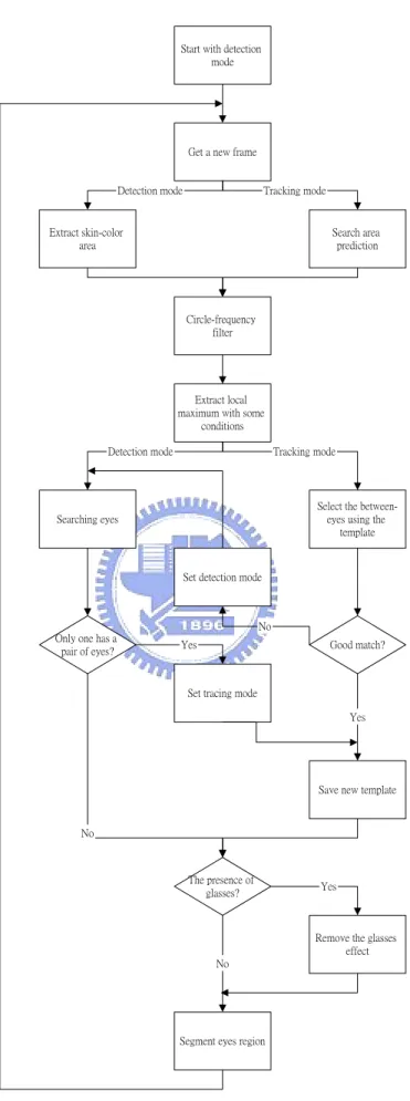
(16) bases on deformable contours. But it is limited in searching of the optimal solution around an initial contour that is close to final solution. Wu et al. [19] introduce a novel example based approach to synthesize an image with glasses removed from the detected and localized face image. They propose a statistical analysis and synthesis approach employing a database containing pairs of face images, one with glasses while the other without. However, it is impossible to have both images of all people to approach this.. In this thesis, we introduce to use edge detection and modified fuzzy rule-based (MFRB) filter [20] for the glasses removal. The glasses removal flow of our system consist three steps: glasses contour extraction, glasses removal, and smoothing by MFRB filter. The first step is to extract the glasses contour by edge detection in RGB, HSV color spaces, and color edge detection [21] in order to segment the glasses contour. Then, each glasses pixel is replaced by its neighborhood in linear increasing or decreasing variation based on its tendency. Finally, use the trained MFRB filter to smooth the glasses region and make it more nature. The MFRB filter is a weighted average of the center pixel and its neighboring pixels in a working window. After this processes, the result of glasses removal will be more smooth, natural, and more close to a non-wearing glasses image.. 1.5. Flowchart of Eye Detection and Glasses Removal System. The system starts with the detection mode. After getting a new color frame, a skin-color area is extracted. In the tracking mode, instead of the skin-color area extraction, we select a small area around the previous point of the “between-eyes” for 6.

(17) the search area, and the remaining processes are restricted to this area. Fig 1.1 shows a flowchart of eye detection system.. In the detection mode, eyes are searched for each candidate. When only one candidate has a pair of eyes, the system assumes it is the “between-eyes”, and switches to the tracking mode after saving a small area around it as a template. Otherwise, it assumes that the detection failed and goes to the next frame.. In the tracking mode, each candidate is compared with the template, and the best match is selected. If it satisfies predefined matching criteria, the system assumes it is the “between-eyes,” and the template is updated. Otherwise, it assumes the “between-eyes” is lost, and switches to the detection mode.. In both detecting and tracking modes, the detection of glasses is produced. For a drowsiness detection system, the effect of eyeglasses is removed such that eye features can be measured accurately, while for a face recognition system, the eyeglasses is removed from the face such that we can recognize the face in the non-wearing glasses facedatabase.. 1.6. Thesis Outline. The thesis is organized as follows. Chapter 2 introduces the face detection algorithm and gives an example. Chapter 3 shows how we use circle-frequency filter to locate the eyes position, and how we detect the presence of glasses. The technique that we use different color models to derive rough glasses edge, locate the eyes region 7.

(18) while one wearing glasses, and glasses removal will also be shown in this chapter. A number of results of each topic of chapters will be given in Chapter 4. We conclude this paper with a discussion in Chapter 5.. 8.

(19) Start with detection mode. Get a new frame. Detection mode. Tracking mode. Extract skin-color area. Search area prediction. Circle-frequency filter. Extract local maximum with some conditions Detection mode. Tracking mode. Select the betweeneyes using the template. Searching eyes. Set detection mode. No Only one has a pair of eyes?. Yes. Good match?. Set tracing mode Yes. Save new template. No. The presence of glasses?. Yes. Remove the glasses effect No. Segment eyes region. Fig 1.1.. Flowchart of eye detection and glasses removal system. 9.

(20) Chapter 2. Face Segmentation. 2.1. Introduction. The task of locating a person’s position in an image taken by a CCD camera is the first step of identifying all human-related activities, such as video surveillance, human computer interface, face recognition, and face image database management. Here we adopt a method proposed by Chai et al. [3]. This method involves a fast, reliable, and effective algorithm that exploits the spatial distribution characteristics of human skin color. Based on the spatial distribution of the detected skin-color pixels and their corresponding luminance values, the algorithm employs a set of novel regularization processes to reinforce regions of skin-color pixels that are more likely to belong to the facial regions and eliminate those that are not.. In this thesis, we use only four stages of the method described above except the luminance regularization stage. The luminance regularity property is only appropriate for a simple background, but we want to identify a person’s face in an image without any constraints. Instead of this stage, we use more constraints on geometry to distinguish the face region and background.. 10.

(21) 2.2. Color Analysis. For recent surveys, face detection utilizes techniques such as principal component analysis, neural network, machine learning, information theory, geometrical modeling, (deformable) template matching, Hough transform, motion extraction, and color analysis. Among all these methods, color analysis is a straightforward method and useful cue for face detection. Some recent publications that have reported this study [3]–[5], [9] also tell us that color are a powerful descriptor and has practically used in the extraction of face location.. Color is perceived by humans as a combination of tristimuli R (red), G (green), and B (blue) (RGB) which are usually called three primary colors. From the RGB representation, we derive other kinds of color representations (space) by using either linear or nonlinear transformations. Several color spaces, such as RGB, HSV, YCrCb, and CIE color spaces are utilized in color image segmentation but none of them can dominate the others for all kinds of color images. Selecting the best color space still is one of the difficulties in color image segmentation.. Here are the brief summaries about the properties of some color spaces that we usually meet. z RGB: This stands for the three primary colors: red, green, and blue. It is a hardware-oriented model and is well known for its color-monitor display purpose. z HSV: An acronym for hue-saturation-value. Hue is a color attribute that describes a pure color; saturation defines the relative purity or the amount of white light mixed with a hue; value refers to the brightness of the image. This 11.

(22) model is commonly used for image analysis. z YCrCb: This is yet another hardware-oriented model. However, unlike the RGB space, here the luminance is separated from the chrominance date. The Y value represents the luminance (or brightness) component, while the Cr and Cb values, also known as the color difference signals, represent the chrominance component of the image. z CIE space: CIE (Commission International de l’Eclairage) color system was developed to represent perceptual uniformity, and thus meets the psychophysical need for a human observer. It has three primaries denoted as X, Y, and Z. The value of X, Y, and Z can be computed by a linear transformation from RGB tristimulus coordinates. CIE space can control color and intensity information more independently and simply than RGB primary colors. Direct color comparison can be performed based on geometric separation within the color space; therefore, it is especially efficient in the measurement of small color difference.. It is important to choose the appropriate color space for modeling human skin color. What we need to be considered are application and effectiveness. Besides, the intended purpose of the face segmentation will usually determine which color space to use; at the same time, it is essential that an effective and robust skin-color model can be derived from the given color space. The reason of using the YCrCb color space is twofold. First, an effective use of the chrominance information for modeling human skin color can be achieved in this color space. Second, this format is typically used in video coding, and therefore the use of the same, instead of another, format for segmentation will avoid the extra computation required in conversion. On the other hand, other methods have opted for the HSV color space, as it is compatible with 12.

(23) human color perception, and the hue and saturation components have been reported also to be sufficient for discriminating color information for modeling skin color. However, this color space is not suitable for video coding.. It is worthy to notice that unlike the YCrCb and HSV color spaces, whereby the brightness component is decoupled from the color information of the image, in the RGB color space it is not. Therefore, it has suggested preprocessing calibration in order to cope with unknown lighting conditions. From this point of view, the skin-color model derived from the RGB color space will be inferior to those obtained from the YCrCb or HSV color spaces. Based on the same reasoning, we hypothesize that a skin-color model can remain effective regardless of the variation of skin color (e.g., black, white, or yellow) if the derivation of the model is independent of the brightness information of the image.. 2.3. Face Segmentation Algorithm. The algorithm in [3] is an unsupervised segmentation algorithm, and hence no manual adjustment of any design parameter is needed in order to suit any particular input image. The only principal assumption is that the person’s face must be present in the given image, since we are locating and not detecting whether there is a face. In this thesis, we do not use the luminance regularization of stage four in Chai et al. [3] proposed algorithm. It is because we do not give any constraint to our background, it may be complex. The luminance regularization which uses the characteristic that the brightness is more non-uniform throughout the facial than background is more likely to use in a simple background situation. The algorithm we use is consists of four 13.

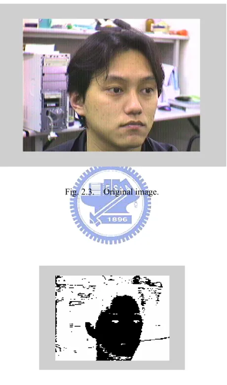
(24) stages, as outlined in Fig. 2.1.. A.. Color Segmentation. The first stage of the algorithm is to classify the pixels of the input image to skin region and non-skin region. To do this, we reference a skin-color reference map in YCrCb color space. The transformation from RGB color space to YCrCb color space is given as follows.. Y = 0.2999R + 0.587G + 0.114B Cb = à 0.169R à 0.331G + 0.500B Cr = 0.500R à 0.419G à 0.081B. (2.1). It has been proved that a skin-color region can be identified by the presence of a certain set of chrominance values (i.e., Cr and Cb) narrowly and consistently distributed in the YCrCb color space. The location of these chrominance values has been found and can be illustrated using the CIE chromaticity diagram as shown in Fig. 2.2. We denote RCr and RCb as the respective ranges of Cr and Cb values that correspond to skin color, which subsequently define our skin-color reference map. The ranges that the paper uses to be the most suitable for all the input images that they have tested are RCr = [133, 173] , and RCb = [77, 127] .. The size of image we use is 320×240. In order to reduce the computing time, we sample the image to become 160×120 and recover in the last stage. Now, consider an image of M×N pixels and we down sample to M/2×N/2. With the skin-color reference map, we got the color segmentation result OA as. 14.

(25) ú. 1, OA(x, y) = 0,. T if [C r (x , y ) ∈ R C r ] [C b (x , y ) ∈ R C b] otehrwise. (2.2). where x = 0, … , M/2-1 and y = 0, … , N/2-1 and M, N are the height and width of the picture respectively. An example to illustrate the classification of the original image Fig. 2.3 is shown in Fig. 2.4.. Among all the stages, this first stage is the most vital. Based on the model of human skin color, the color segmentation has to remove as many pixels as possible that are unlikely to belong to the facial region while catering for a wide variety of skin color. However, if it falsely removes too many pixels that belong to the facial region, then the error will propagate down the remaining stages of the algorithm, consequently causing a failure to the entire algorithm.. Nevertheless, the result of color segmentation is the detection of pixels in a facial area and may also include other areas where the chrominance values coincide with those of the skin color (as is the case in Fig. 2.4). Hence the successive operating stages of the algorithm are used to remove these unwanted areas.. B.. Density Regularization. This stage considers the bitmap produced by the previous stages to contain the facial region that is corrupted by noise. The noise may appear as small holes on the facial region due to undetected facial features such as eyes, mouth, even glasses, or it may also appear as objects with skin-color appearance in the background scene.. 15.

(26) Input Image: An Image Including A Face. Color Segmentation. Density Regularization. Geometric Correction. Contour Extraction. Output Image: Segmented Facial Region Fig. 2.1.. Outline of face-segmentation algorithm.. Chrominance values found in facial region Fig. 2.2.. Skin-color region in CIE chromaticity diagram. 16.

(27) Fig. 2.3.. Fig. 2.4.. Original image.. Image after filtered by skin-color map in stage A.. 17.

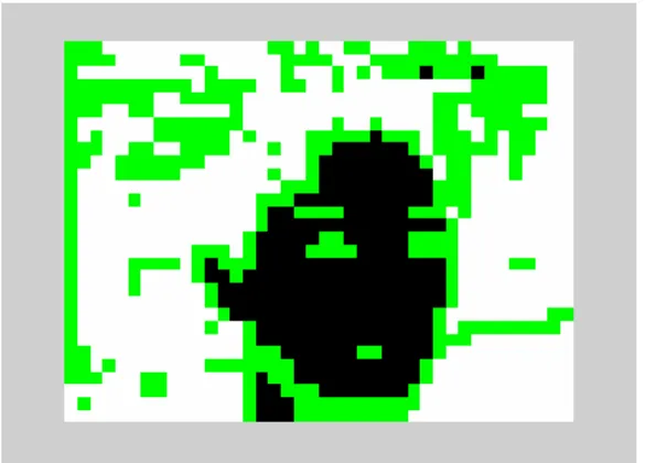
(28) Therefore, this stage performs simple morphological operations such as dilation to fill in any small hole in the facial area and erosion to remove any small object in the background area. The intention is not necessarily to remove the noise entirely but to reduce its amount and size.. To distinguish between facial and non-facial region, we first need to identify regions of the bitmap that have higher probability of being the facial region. The probability measure that we used is derived from our observation that the facial color is very uniform, and therefore the skin-color pixels belonging to the facial region will appear in a large cluster, while the skin-color pixels belonging to the background may appear as large clusters or small isolated objects. Thus, we study the density distribution of the skin-color pixels detected in stage A. A density map is calculus as follows. 3 P 3 à á P à á D x, y = O A 4x + i, 4y + j i=0 j=0. (2.3). It first partitions the output bitmap of stage A OA(x, y) into non-overlapping groups of 4×4 pixels, then counts the number of skin-color pixels within each group and assigns this value to the corresponding point of the density map.. According to the density value, we classify each point into three types, namely, zero (D = 0), intermediate (0 < D < 16), and full (D = 16). A group of points with zero density value will represent a non-facial region, while a group of full density points will signify a cluster of skin-color pixels and a high probability of belonging to a facial region. Any point of intermediate density value will indicate the presence of noise. The density map of an example with three density classifications is depicted in Fig. 2.5. The point of zero density is shown in white, intermediate density in green, 18.

(29) and full density in black.. Once the density map is derived, we can then begin the process that we termed as density regularization. This involves the following three steps. 1). Discard all points at the edge of the density map, i.e., set D(0, y) = D(M/8-1, y) = D(x, 0) = D(x, N/8-1) for all x = 0, …, M/8-1 and y = 0, …, N/8-1.. 2). Erode any full-density point (i.e., set to zero) if it is surrounded by less than five other full-density points in its local 3×3 neighborhood.. 3). Dilate any point of either zero or intermediate density (i.e., set to 16) if there are more than two full-density points in its local 3×3 neighborhood.. After this process, the density map is converted to the output bitmap of stage B as ú 1, OB(x, y) = 0,. if D (x , y ) = 16 otherwise. for all x = 0, …, M/8-1 and y = 0, …, N/8-1.. The result of the previous example is displayed in Fig. 2.6.. Fig. 2.5.. Density map after classified to three classes. 19. (2.4).

(30) Fig. 2.6. Image produced by stage B.. C.. Geometric Correction. We performed a horizontal and vertical scanning process to identify the presence of any odd structure in the previously obtained bitmap, OB(x, y), and subsequently removed it. This is to ensure that a correct geometric shape of the facial region is obtained. However, prior to the scanning process, we will attempt to further remove any more noise by using a technique similar to that initially introduced in stage B. Therefore, a pixel in OB(x, y) with the values of one will remain as a detected pixel if there are more than three other pixels, in its local 3×3 neighborhood, with the same value. At the same time, a pixel in OB(x, y) with a value of zero will be reconverted to a value of one (i.e., as a potential pixel of the facial region) if it is surrounded by more than five pixels, in its local 3×3 neighborhood, with a value of one. These simple procedures will ensure that noise appearing on the facial region is filled in and that isolated noise objects on the background are removed.. We then commence the horizontal scanning process on the “filtered” bitmap. We search for any short continuous run of pixels that are assigned with the value of one. For a CIF-size image, the threshold for a group of connected pixels to belong to the 20.

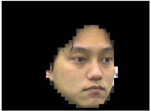
(31) facial region is four. Therefore, any group of less than four horizontally connected pixels with the value of one will be eliminated and assigned to zero. A similar process is then performed in the vertical direction. The rationale behind this method is that, based on our observation, any such short horizontal or vertical run of pixels with the value of one is unlikely to be part of a reasonable-size and well-detected facial region. As a result the output bitmap of this stage should contain the facial region with minimal or no noise, as demonstrated in Fig. 2.7.. D.. Contour Extraction. In this final stage, we convert the M/8×N/8 output bitmap of stage C back to the dimension of M/2×N/2. To achieve the increase in spatial resolution, we utilize the edge information that is already made available by the color segmentation in stage A. Therefore, all the boundary points in the previous bitmap will be mapped into the corresponding group of 4×4 pixels with the value of each pixel as defined in the output bitmap of stage A. The representative output bitmap of this final stage of the algorithm is shown in Fig. 2.8.. Fig. 2.7. Image produced by stage C.. 21.

(32) Fig. 2.8. Image produced by stage D.. 22.

(33) Chapter 3. Eye Detection and Glasses Removal. 3.1. Introduction to Eye Detection. The face location problem in image sequences has been solved using skin-color information in Chapter 2. After locating a face area, we try to extract the eye region such that we could measure eye features for applications. Some techniques are proposed to find the eye position such as threshold technique and candidate matching. However, these methods seem not robust against the orientation and scale variation of face images. For the general purpose to every user without database and the robustness for lighting condition and orientation, we adopt the method proposed by Kawato et al. [16] that use circle-frequency filter to solve these questions.. In [16], it tries to find a candidate “between-eyes” that between the eyes rather than the eyes directly. “Between-eyes” has dark parts on both sides including the eyes and eyebrows, and it is comparably bright in the upper side (forehead) and the lower side (nose bridge). The characteristic seems to be common to most people, and it can be seen for a wide range of face orientations. This paper proposed an image filter, i.e., the circle-frequency filter, to detect “between-eyes.” Although the circle-frequency filter can robustly extract “between-eyes,” many other similar characteristic points are also extracted. By evaluating other local features, however, we can limit these points to one or several points. Then, we look for dark regions as the eyes on both sides of the candidates for “between-eyes”. When only one candidate satisfies certain geometric conditions with a pair of eye like regions, we take this candidate as. 23.

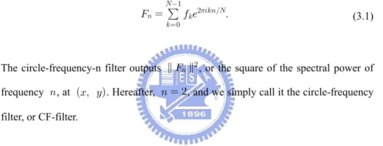
(34) “between-eyes” and the dark region as eyes. Following this, the small area around “between-eyes” is then copied as a template for eye tracking.. 3.2. Circle-Frequency Filter. Assume that fi (i = 0, ..., N à 1) are pixel values along a circle centered at (x, y) . Then, we can calculate their discrete Fourier transform as. Fn =. Nà1 P. fke2ùikn/N.. k=0. (3.1). The circle-frequency-n filter outputs k Fn k2 , or the square of the spectral power of frequency n , at (x, y) . Hereafter, n = 2 , and we simply call it the circle-frequency filter, or CF-filter.. Fig. 3.1 shows an example of fi ’s at “between-eyes” (the green dot at the center). The radius of the blue circle is two-fifths of face width, and 116 pixel values along it are plotted on the graph in this case. The plot starts at the forehead and goes counter clockwise. There are two cycles of dark and bright. The output of the CF-filter for this pattern becomes high, which is known as a characteristic of the Fourier transform. An example of a CF-filtered image is given in Fig. 3.2.. 24.

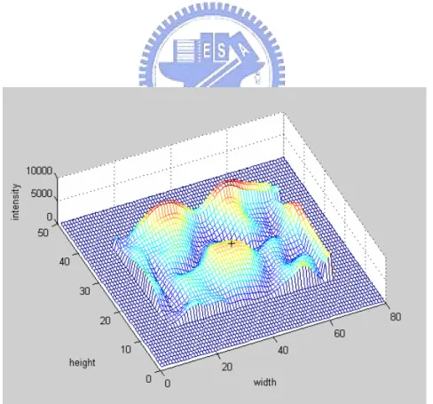
(35) Gray level pixel values Pixel number. (a). (b). Fig. 3.1. An example of “between-eyes” extracted by circle-frequency filter. (a) Between-eyes and the surrounding circle with a radius of two-fifths of face width. (b) The pixel values along the circle which start at the forehead and go counter clockwise.. Fig. 3.2.. The CF-filtered image. The black plus “+” is a local maximum of image. which satisfies the two conditions in Section 3.3.. 25.

(36) 3.3. “Between-Eyes” Candidate Evaluation. First, it uses two conditions to eliminate “between-eyes” candidates. 1.. The left and right pixel values of “between-eyes” on the circle of the filter must be lower than that of “between-eyes” itself.. 2.. The real part of F2 in Eq. (3.1) when n = 2 must be positive, which means that the phase of signal fi begins with a brighter part.. These conditions are reasonable when the face rotation in the image plane is less than 45 degrees. The top three are tested further by confirming eye detection in the detection mode.. After choosing possible candidates, we select the best candidate by locating eyes. At first, rectangular areas on both sides of the “between-eyes” candidate point where the eyes should be found are extracted. The area size is defined in advance. The next step is to find the threshold level for each area to binaries the image. This is done by searching for the level from the lowest level using a connected component analysis. The threshold level is determined when the sum of the number of pixels of all components not on the border of the rectangular area, exceeds a certain value. We avoid components on the border because they often belong to hair. Sometimes, the eyebrows have the same gray level as the eyes. Accordingly, from among the extracted components, we select one component within a certain range of pixels and with the lowest position. Then, the distance between the located eyes ( De ) in pixels and the angle ( Ae ) between the left and right eyes at “between-eyes” are tested as follows. These conditions are defined from experiments.. 31 < De < 42 26. (3.2).

(37) 115 < Ae < 180. (3.3). When only one candidate has a pair of eyes in this condition, we assume it to be “between-eyes,” and the 15×15 pixels around it are copied from the monochrome smoothed image as a template. Otherwise, the “between-eyes” and eye locations are not determined.. 3.4. Tracking “Between-Eyes”. It does not need to extract skin-color areas while “between-eyes” is located in a previous frame. When “between-eyes” is located in only the previous one frame, we predict its position to be the same location in the current frame as in the previous frame. On the other hand, when it is located in the previous two frames, we predict its position as follows. x p = 2x 1 à x 2. (3.4). where xp is the predicted position, and x1 and x2 are the position in the past one and two frames, respectively.. Then, the search area becomes a predefined rectangular area centered at the predicted position, which is converted to a monochrome image, using gray level image. The extracting process of candidates for “between-eyes” is the same as described before, but the selection process is different. Among the candidates, we select the candidate nearest to the predicted position. Then, conformation is done by template matching. The matching index is not a normalized cross correlation but 27.

(38) simply a sum-up of the absolute values of the differences in corresponding pixels.. When the matching index is less than a predefined threshold, the system assumes that “between-eyes” has been lost and switches to the detection mode. Otherwise, the template is updated for the next frame. Therefore, the system can follow changes in the appearance of “between-eyes,” as long as the changes are gradual and the circle-frequency filter can pick the point out as a candidate.. 3.5. Glasses Existence Detection. There are many kinds of glasses, with different materials and different colors. Furthermore, sometimes there is no frame around the eyeglasses. However, the nosepiece is one of the most common features existing on all of the glasses. It is indispensable and very obvious in any kind of glasses. Using this important feature, face images with glasses can be detected.. Using the “between-eyes” and the eyes location information we have found, the region around the “between-eyes” and also the center of the eyes location is the most powerful criterion for glasses detection. The nosepiece can be found in the region where the presence of edges is an important cue. Using a gradient edge detector, we obtain at each point (x, y) the magnitude and the orientation of the gradient as follows:. G=. q G2x + G2y. ,. ò = arctan(Gy/Gx). (3.5). where Gx and Gy are the horizontal and vertical derivatives obtained at the pixel. 28.

(39) (x, y) . Then, if the number of pixels which having a vertical direction exceeds a fixed threshold, the presence of glasses is determined.. 3.6. Eye Location While Wearing Glasses. If the glasses are presence, we have to locate eyes without glasses for measuring the closure of eyes for some specific applications, such as drowsiness detection system. We begin with the region that contains the eyes and glasses. First, we compute the color edge of the eye region in HSV color model and do erosion and dilation to get the rough edge map of glasses. The color edge detection method proposed by Fan et al. [21] use entropic thresholding technique to obtain an optimal threshold that is adaptive to the image contents, and this technique has been proved to be highly efficient for two-class data classification problem [22]. Then, we convert the image of eye region from RGB color space to YCrCb color space. It is easy to see that in YCrCb color model domain, the intervals of the Cr and Cb components of skin-color are always very different from glasses and can easily be clustered to two classes. However, for kinds of glasses, such as metallic and thin-frame, the color of glasses frame sometimes lies in the skin-color interval in YCbCr color model because the metallic reflection and the noise caused by low resolution CCD. In order to deal with these problems, we add extra information of RGB gradient edge detector. Therefore, we combine the three evidences to guarantee that the glasses have completely been extracted, despite some noises caused by hair or eyebrows to be included in the map. Figs. 3.3–3.4 show two examples of edge detection while one worn on two different kinds of glasses.. 29.

(40) After getting the edge map of detected eye region, we use geometry and projections to eliminate the glasses region and locate accurately the eyes position. When we apply erosion to the edge image of wearing glasses image, the edge will break into small pieces and then the eye can be separated from glasses contour easily by selecting the largest connected component which has the smallest standard deviation to each center of the component. The hair and eyebrows components also can be recognize because it is always from the top to the bottom and begin with the top of the eye region we have set. The extracted eye position result from edge map of wearing glasses examples in Figs. 3.3–3.4 demonstrate in Figs. 3.5–3.6. Finally, we can measure the closure of eyes by its vertical length and area, and determine whether the driver is drowsy or not in drowsiness detection using PERCLOS and blinking rate, which are the duration and frequency of eye closure respectively.. 3.7. Glasses Removal. After successfully locating glasses contour, the remaining work we have to do for taking off the camouflage of face recognition system is replacing the pixels on glasses segment by skin-color pixels. Although we can just replace it by its neighborhood pixel values, it will be seen to be very rough and unnatural. In order to make the recovered images more natural, we use the modified fuzzy rule-based (MFRB) filter [20] to re-smooth the glasses pixels and make them more close to a non-wearing glasses image. A fuzzy rule-based (FRB) image filter introduced by Arakawa [23] is realized as a weighted-averaging-type filter in which the values of the weights are controlled based on the fuzzy rules, in order to take the ambiguity of signals into consideration. Here we adopt three rules: the first is the difference 30.

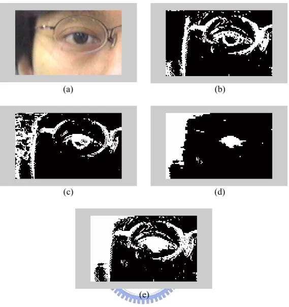
(41) (a). (b). (c). (d). (e) Fig. 3.3.. First example of edge detection. (a) Original image. (b) Edge detection. using gradient operator in RGB color space with dilation. (c) Edge detection using gradient operator in Hue component of HSV color space with dilation. (d) Non-skin-color region. (e) The resultant edge map union the previous three edge map.. 31.

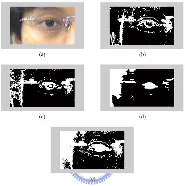
(42) (a). (b). (c). (d). (e) Fig. 3.4.. Second example of edge detection. (a) Original image. (b) Edge detection. using gradient operator in RGB color space with dilation. (c) Edge detection using gradient operator in Hue component of HSV color space with dilation. (d) Non-skin-color region. (e) The resultant edge map union the previous three edge map.. 32.

(43) Fig. 3.5. (a). (b). (c). (d). Eye extraction from edge map of Fig. 3.3. (a) Edge map of eye region. (b). Edge map with eliminating the hair region. (c) Edge map which eliminating hair region with twice erosion. (d) Extraction the pupil position.. Fig. 3.6. (a). (b). (c). (d). Eye extraction from edge map of Fig. 3.4. (a) Edge map of eye region. (b). Edge map with eliminating the hair region. (c) Edge map which eliminating hair region with twice erosion. (d) Extraction the pupil position. 33.

(44) between the input signal values; the second is the time distance between signal points, and the third is the local variance in the filter window. This is because that these three factors have strongly influenced the pixel from its neighborhood. Usually in fuzzy-rule-based systems, the membership functions for the input parameters must be given beforehand; however, in this proposal the membership functions are generated automatically by a learning method. Before using MFRB filter to smooth, we replace the pixel values of glasses contour by its neighborhood in increasing or decreasing variation according to its tendency in Y component of YCrCb color space. Figs 3.7–3.8 show two examples that pixel values of glasses contour have been replaced using the method described above. And then, the weights are obtained so that they minimize the mean square error of typical examples of wearing glasses images that the glasses contour has been substituted using the rule explained previously and non-wearing glasses images.. Suppose that a noisy signal xn is obtained at time point n as xn = dn + un , where dn denotes an original signal and un a white Gaussian noise with zero mean. A filter to estimate the value of dn can be expressed as follows. yn =. N P. ö n;nàkxnàk. k=àN N P. .. (3.6). ö n;nàk. k=àN. Here, yn denotes the estimated value of dn and ön;nà k the weight which represents to what extent the input xnàk should be used in the weighted average to get the estimation of dn .. 34.

(45) (a). (b). (c) Fig. 3.7.. First example of replacing the glasses contour by its neighborhood. (a). Original image. (b) Edge map. (c) resultant image.. (a). (b). (c) Fig. 3.8.. Second example of replacing the glasses contour by its neighborhood. (a). Original image. (b) Edge map. (c) resultant image.. 35.

(46) In order to set the value of ön;nàk based on multiple rules, ön;nàk should be expressed as a multidimensional function of the parameters used in the rules. When the above three rules are applied, ön;nàk should be expressed as a function of these three parameters, the signal difference xn à xn à k , the time distance k , and the local variance ûn , as ö(sn;nàk, k, ûn) . Here xn à xn à k is denotes as sn;nàk for short. The function ö(sn;nàk, k, ûn) is expressed as öjkm at the j th, the k th, and the. mth step for sn;nàk , k , and ûn , respectively. Then the value öjkm can be obtained for all the combination of j, k , and m by the LMS algorithm iteratively as follows, so that the mean square error of the filter output for some known training signals can be the minimum. öjkm(n + 1) = öjkm(n) + ëtjkm(xnàk à yn) á (dn à yn)/. N P. öjkm(n) .. (3.7). k=àN. Here, öjkm(n) is the value of öjkm at time point n , ë a factor for the stability and convergence, and tjkm is a value as follows for the input xnàk at time point n. ú 1, tjkm = 0,. if εj à1 ô s n;nàk < εj otherwise.. (3.8). εj and εm are the parameters to divide the values of sn;nàk and ûn into pieces. Eq.. (3.8) is repeated until öjkm(n) converges.. An example of training data is given in Fig. 3.9, (a) is the image in which a person wearing glasses, (b) is the result of glasses contour (white pixels), (c) is the image that the detected glasses contour pixels have been recovered by its neighborhood pixel values, and (d) is the non-wearing glasses image from the same person. Here we only train the pixels in the glasses contour. Pixel values in. 36.

(47) non-wearing glasses image is supposed to be estimated value yn , while in wearing glasses image to be noisy signal xn . The initial membership function öjkm (0) is decreasing from 1 to 0 as j, k, and m increasing. Fig 3.10 shows an example after MFRB filtering, where (a) is the result of Fig. 3.9(c) after MFRB filter processing, and (e) is the image in which the same person who do not wear glasses. A comparison of images with and without smoothing by MFRB filter is given in Fig. 3.11.. Fig. 3.9.. (a). (b). (c). (d). Example of training data. (a) The image in which a person wearing glasses.. (b) The result of glasses contour. (c) The image that the detected glasses contour pixel values have been recovered by its neighborhood pixel values. The training data is the pixels of the glasses contour (white part in (b)) which its 3×3 neighborhood are all pixels of glasses segment. (d) The image of the same person who do not wear glasses. 37.

(48) (a). Fig. 3.10.. (b). Result of Fig. 3.9 after MFRB filtered. (a) The result of Fig. 3.9(c) after. MFRB filter processing. (b) The image of the same person who do not wear glasses.. (a). (b) Fig. 3.11.. A comparison that with and without smoothing by MFRB filter. (a) Image. without smoothing by MFRB filter. (b) Image with smoothing by MFRB filter.. 38.

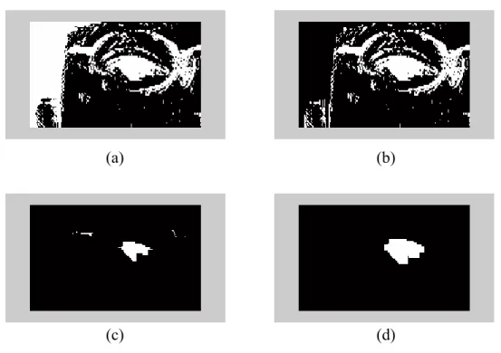
(49) Chapter 4. Simulation and Results. The eye-detection algorithm was tested on a number of people in order to confirm the validity. First, we capture frontal face images of people by a CCD camera, and then we will validate the algorithm via these images. In Section 4.1, the algorithm will be tested of people who do not wearing glasses. We will give the step-by-step result of finding the eyes. On the other hand, wearing glasses cases will be examining in Section 4.2. The size of images is 640×480 and the simulation is processing on a Pentium IV 2.4GHz personal computer.. 4.1 Non-Wearing Glasses Cases We take frontal face images of four students in laboratory to test the eye extraction algorithm. Figs. 4.1– 4.4 show these four examples. In each example, we will show the original face image in sub-image (a), and face extraction result in (b). The input and output images of circle-frequency filter (CF-filter) are given in sub-image (c) and (d) respectively. Sub-image (e) shows the “between-eyes” on face with surrounding circular pixels, while (f) shows the eye extraction result. The accuracy of the result for finding eye location is 100%.. 39.

(50) Fig. 4.1.. (a). (b). (c). (d). (e). (f). Images of example 1 for face detection and eye location. (a) The input. image. (b) Face extraction result. (c) The input image for CF-filter. (d) The output of CF-filter. (e) The “between-eyes” location. (f) The eye region.. 40.




(54) 4.2. Wearing Glasses Cases In this section, we will represent our glasses removal technique using edge. detection and MFRB filter. The eye extraction algorithm is also applicable for wearing-glasses cases. Figs. 4.5–4.7 are the three examples of eight training data for training the membership function of MFRB filter. The testing data are four students wearing on three different glasses at random. Here we will show the intermediate processing steps in Figs. 4.8–4.9. Figs. 4.10–4.13 give others examples comparing with non-wearing glasses case. In chromatic glasses removal image of these examples, the Y component of YCrCb color space of each glasses pixel is computed as we described above, and the Cr and Cb components are replacing by the average pixel values in skin-color around the glasses.. Fig. 4.5.. (a). (b). (c). (d). An example of training data. (a) The image in which a person wearing. glasses. (b) The result of glasses contour. (c) The image that the detected glasses contour pixel values have been recovered by its neighborhood pixel values. The training data is the pixels of the glasses contour (white region in (b)), in which each pixel associated with its 3×3 neighborhood are all pixels of glasses segment. (d) The non-wearing glasses image from the same person. 44.

(55) (a). (b). (c). (d). Fig. 4.6. Second example of training data. (a) The image in which a person wearing glasses. (b) The result of glasses contour. (c) The image that the detected glasses contour pixel values have been recovered by its neighborhood pixel values. The training data is the pixels of the glasses contour (white region in (b)), in which each pixel associated with its 3×3 neighborhood are all pixels of glasses segment. (d) The non-wearing glasses image from the same person.. (a). (b). (c). (d). Fig. 4.7. Third example of training data. (a) The image in which a person wearing glasses. (b) The result of glasses contour. (c) The image that the detected glasses contour pixel values have been recovered by its neighborhood pixel values. The training data is the pixels of the glasses contour (white region in (b)), in which each pixel associated with its 3×3 neighborhood are all pixels of glasses segment. (d) The non-wearing glasses image from the same person. 45.

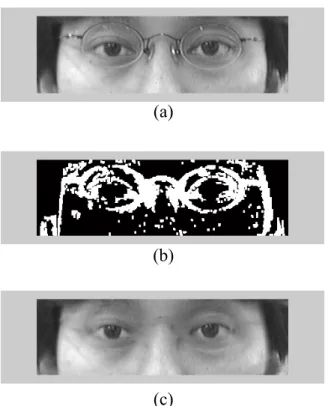
(56) Fig. 4.8.. (a). (b). (c). (d). (e). (f). (g). (h). An example for glasses removal details. (a) The wearing glasses image. (b). The non-wearing glasses image. (c) The eye location of (a). (d) The edge of glasses in (c). (e) The result of glasses removal of (c) in gray level. (f) The result of (c) after MFRB filtering. (g) The result of glasses removal of (a) in gray level. (h) The result of glasses removal of (a) in chromatic levels.. 46.

(57) Fig. 4.9.. (a). (b). (c). (d). (e). (f). (g). (h). Second example for glasses removal details. (a) The wearing glasses image.. (b) The non-wearing glasses image. (c) The eye location of (a). (d) The edge of glasses in (c). (e) The result of glasses removal of (c) in gray level. (f) The result of (c) after MFRB filtering. (g) The result of glasses removal of (a) in gray level. (h) The result of glasses removal of (a) in chromatic levels.. 47.

(58) (a). (b). (c). (d). (e). (f). Fig. 4.10. First example of glasses removal algorithm. (a) and (b) are a wearing glasses example in gray level and RGB color space respectively, (c) and (d) are results of processing with glasses removal algorithm in gray level and chromatic levels respectively, (e) and (f) are the corresponding non-wearing glasses case of (a) and (b) in gray level and chromatic levels. 48.

(59) (a). (b). (c). (d). (e). (f). Fig. 4.11. Second example of glasses removal algorithm. (a) and (b) are a wearing glasses example in gray level and RGB color space respectively, (c) and (d) are results of processing with glasses removal algorithm in gray level and chromatic levels respectively, (e) and (f) are the corresponding non-wearing glasses case of (a) and (b) in gray level and chromatic levels. 49.

(60) (a). (b). (c). (d). (e). (f). Fig. 4.12. Third example of glasses removal algorithm. (a) and (b) are a wearing glasses example in gray level and RGB color space respectively, (c) and (d) are results of processing with glasses removal algorithm in gray level and chromatic levels respectively, (e) and (f) are the corresponding non-wearing glasses case of (a) and (b) in gray level and chromatic levels. 50.

(61) (a). (b). (c). (d). (e). (f). Fig. 4.13. Fourth example of glasses removal algorithm. (a) and (b) are a wearing glasses example in gray level and RGB color space respectively, (c) and (d) are results of processing with glasses removal algorithm in gray level and chromatic levels respectively, (e) and (f) are the corresponding non-wearing glasses case of (a) and (b) in gray level and chromatic levels. 51.

(62) Chapter 5. Conclusion. In this thesis, eye detection and glasses removal algorithm is developed to localize the eye region and remove the glasses from faces while the glasses is present on faces. The applications we are interested in are drowsiness detection system that provides an early detection and warning of fatigue at the wheel. Glasses removal can also provide face recognition system in taking off the camouflage when one wears eyeglasses.. Our system first uses the universal skin-color map to detect the face region and CF-filter to locate the “between-eye.” The eye regions can be determined in advance according to “between-eyes”. Then, if there present glasses on face, a glasses removal algorithm, which is based on edge detection and MFRB filter, is used to find the eye except the glasses and remove the glasses. The main features we used to obtain the contour of glasses are edge detection algorithm performed in HSV, RGB color space, and color edge detection. After obtaining the glasses contour, we replace the contour pixel values by its neighborhood pixel value in increasing or decreasing variation based on its tendency. Finally, MFRB filter is exploited to refine the pixel values in the glasses region.. Through our algorithms, slight head rotation and different head orientation are acceptable. For a wearing glasses case, the glasses removal algorithm gives a solution to separate the eyes and glasses such that we can find the eye and determine the eye closure more accurate. Furthermore, glasses removal results, as shown in Section 4.2, have demonstrated the effectiveness of our method. In the simulation results, the 52.

(63) accuracy rates of face detection and “between-eyes” location on our testing data are both 100% whether wearing glasses or not. The eye location accuracy in wearing glasses cases of our testing data is also 100% with some limitations below. First, if the glasses cross edges of eyes, the eye location will be interfered and hence eyes and glasses will overlap and it may be difficult to separate the eyes from glasses. Second, in the glasses removal process, eyebrows or eyes cross edges of glasses creating substantial ambiguities. Moreover, when the pixel values of glasses and skin-color are very similar in HSV and YCrCb color models, it will cause similar problem.. For future work, we shall use deformable contour to locate the glasses more accurately and reduce the non-glasses regions that have been error detected. We also try to solve the noise caused by shadows, light reflection of lenses and frames of metallic glasses, and the overlapping of eyes, eyebrows, and glasses.. 53.

(64) References [1]. Y. C. Chiu and J. Y. Chang, “The drowsiness detection for intelligent transport system,” thesis from the Department of Electrical and Control Engineering of National Chiao Tung University in Taiwan, 2003.. [2]. E. Hjelmas and B. K. Low, “Face detection: A survey,” Computer Vision and Image Understanding, vol. 83, pp. 236–274, 2001.. [3]. D. Chai and K. N. Ngan, “Face segmentation using skin-color map in videophone applications,” IEEE Trans. Circuits Syst. Video Technol., vol. 9, pp. 551–564, 1999.. [4]. R. L. Hsu, M. A. Mottaleb, and A. K. Jain, “Face detection in color images,” IEEE Trans. Pattern Anal. Machine Intell., vol. 24, pp. 696–706, 2002.. [5]. H. Wu, Q. Chen, and M. Yachida, “Face detection from color images using a fuzzy pattern matching method,” IEEE Trans. Pattern Anal. Machine Intell., vol. 21, pp. 557–563, 1999.. [6]. J. Yang and A. Waibel, “A real-time face tracker,” in Proc. 3rd IEEE Workshop on Application of Computer Vision, 1996, pp. 142–147.. [7]. R. Féraud, O. J. Bernier, J. E. Viallet, and M. Collobert, “A fast and accurate face detection based on neural network,” IEEE Trans. Pattern Anal. Machine Intell., vol. 23, pp. 42–53, 2001.. [8]. D. Maio and D. Maltoni, “Real-time face location on gray-scale static images,” Pattern Recognition, vol. 33, pp. 1525–1539, 2000.. [9]. C. Garcia and G. Tziritas, “Face detection using quantized skin color regions merging and wavelet packet analysis,” IEEE Trans. Multimedia, vol. 1, pp. 264–27, 1999.. [10]. K. K. Sung and T. Poggio, “Example-based learning for view-based human face detection,” IEEE Trans. Pattern Anal. Machine Intell., vol. 20, pp. 39–51, 1998. 54.

(65) [11] K. C. Yow and R. Cipolla, “Feature-based human face detection,” Image and Vision Computing, vol. 15, pp. 713–735, 1997. [12]. S. A. Sirohey and A. Rosenfeld, “Eye detection in a face image using linear and nonlinear filters,” Pattern Recognition, vol. 34, pp. 1367–1391, 2001.. [13]. G. C. Feng and P. C. Yuen, “Multi-cues eye detection on gray intensity image,” Pattern Recognition, vol. 34, pp. 1033–1046, 2001.. [14]. R. Thilak Kumar, S. Kumar Raja, and A. G. Ramakrishnan, “Eye detection using color cues and projection functions,” in Proc. IEEE Int. Conf. Image Processing, 2002, vol. 3, pp. 24–28.. [15] Z. Liu, X. He, J. Zhou, and G. Xiong, “A novel method for eye region detection in gray-level image,” in Proc. IEEE Int. Conf. Communications, Circuits and Systems and West Sino Expositions, 2002, vol. 2, pp. 1118–1121. [16]. S. Kawato and J. Ohya, “ Two-step approach for real-time eye tracking with a new filtering technique,” in Proc. IEEE Int. Conf. Syst., Man, Cybern., 2000, vol. 2, pp. 1366–1371.. [17]. X. Jiang, M. Binkert, B. Achermann, and H. Bunke, “Towards detection of glasses in facial images,” in Proc. 14th Int. Conf. Pattern Recognition, 1998, vol. 2, pp. 1071–1073.. [18]. Z. Jing and R. Mariani, “Glasses detection and extraction by deformable contour,” in Proc. 15th Int. Conf. Pattern Recognition, 2000, vol. 2, pp. 933–936.. [19]. C. Wu, C. Liu, H. Y. Shum, Y. Q. Xu, and Z. Zhang, “Automatic eyeglasses removal from face images,” in Proc. 5th Asia Conf. Computer Vision, 2002, pp. 23–25.. [20]. J. Y. Cheng and S. M. Lu, “Image blocking artifact suppression by the modified fuzzy rule-based filter,” in Proc. IEEE Int. Conf. Syst., Man., Cybern., 2003, vol. 1, pp. 486–491.. 55.

(66) [21] J. Fan, D. K. Y. Yau, A. K. Elmagarmid, and W. G. Aref, “Automatic image segmentation by integrating color-edge extraction and seeded region growing,” IEEE Trans. Image Processing, vol. 10, pp. 1454–1466, 2001. [22]. J. Fan, R. Wang, L. Zhang, D. Xing, and F. Gan, “Image sequence segmentation based on 2-D temporal entropy,” Pattern Recognition Lett., vol. 17, pp. 1101–1107, 1996.. [23]. K. Arakawa, “Fuzzy rule-based signal processing and its application to image restoration,” IEEE J. Select. Areas Commun., vol. 12, pp. 1495–1502, 1994.. 56.

(67)