PII: S0301-5629(00)00323-9
●
Original Contribution
A TEXTURAL APPROACH BASED ON GABOR FUNCTIONS FOR
TEXTURE EDGE DETECTION IN ULTRASOUND IMAGES
C
HUNG-M
INGC
HEN,* H
ENRYH
ORNG-S
HINGL
U,
†and K
O-C
HUNGH
AN*
*Institute of Biomedical Engineering, National Taiwan University, Taipei, Taiwan; and†Institute of Statistics, National Chiao-Tung University, Hsin-Chu, Taiwan
(Received 20 April 2000; in final form 12 September 2000)
Abstract—Edge detection is an important, but difficult, step in quantitative ultrasound (US) image analysis. In this paper, we present a new textural approach for detecting a class of edges in US images; namely, the texture edges with a weak regional mean gray-level difference (RMGD) between adjacent regions. The proposed approach comprises a vision model-based texture edge detector using Gabor functions and a new texture-enhancement scheme. The experimental results on the synthetic edge images have shown that the performances of the four tested textural and nontextural edge detectors are about 20%–95% worse than that of the proposed approach. Moreover, the texture enhancement may improve the performance of the proposed texture edge detector by as much as 40%. The experiments on 20 clinical US images have shown that the proposed approach can find reasonable edges for real objects of interest with the performance of 0.4ⴞ 0.08 in terms of the Pratt’s figure. (E-mail: [email protected]) © 2001 World Federation for Ultrasound in Medicine & Biology.
Key Words: Ultrasound image, Edge detection, Early vision model, Wavelet analysis, Distance map, Difference
mask.
INTRODUCTION
Edge detection is an essential task in many quantitative analyses of ultrasound (US) images. It usually serves as the first step in border identification, area and volume measurement for the object of interest. Some typical examples are border detection of hepatic ducts (Sun et al. 1996), contour detection of breast tumors (Collaris and Hoecks 1996), contour tracking of cardiac structures (Chalana et al. 1996; Mikic et al. 1998), tongue contour tracking (Akgul et al. 1999), and so on. Nevertheless, edge detection has been recognized as a difficult problem in US image analysis due to the intrinsic noisy and textural nature of a US image.
The intrinsic noises and textures result from such factors as signal processing, image formation, interpola-tion, tissue property, speckle, artefact, and so forth. The most notorious phenomenon is the speckle, which de-grades not only the perceivable resolution by a factor of 5 to 7 (Kozma and Christensen 1976), but also the discriminability of subtle difference in grey levels
(George et al. 1976). The texture pattern, composed of quasirepetitive texcels (i.e., texture elements) or sporadic spots of middle-grained size, basically reflects the tissue property. It should be pointed out that the speckles, textures and artefacts are considered as noises primarily from the viewpoint of edge detection. For practical clin-ical applications, speckles, textures and artefacts fre-quently play an important role in making the diagnosis. The fundamental difficulty of US image edge de-tection mainly arises from the false edges that are easily generated from the speckles, texcels, sporadic spots and artefacts. An edge of an object of interest in an US image is intrinsically determined by two properties of the two adjacent regions forming the edge. One property is the regional mean grey-level difference (RMGD) (i.e., the difference of the mean grey levels of these two regions). The other property is the texture difference of these two regions. If the RMGD is significant, regardless of the texture difference, the edge may be easily detected by classic approaches because the strength of the desired edge is much stronger than that of false edges.
However, for many US image applications, such as hepatic tumor analysis, it is quite common that the RMGD of the desired edge is not significant enough, which has made edge detection a hard problem because Address correspondence to: Chung-Ming Chen, Institute of
Bio-medical Engineering, College of Medicine, National Taiwan Univer-sity, #1, Sec. 1, Jen-Ai Road, Taipei, Taiwan. E-mail: chung@ lotus.mc.ntu.edu.tw
Printed in the USA. All rights reserved 0301-5629/01/$–see front matter
determination of the desired edges may be seriously interfered with by the false edges. What is even worse is that, in the extreme case, the desired edge may be pri-marily defined by the texture difference. It means that those edge-detection approaches designed to utilize the RMGD would be ineffective or even useless in capturing these edges. Because the texture of the object of interest normally differs from that of its surrounding tissues, this paper would focus on finding the texture edges with a weak RMGD. A textural edge is defined as an edge formed by two regions with different texture patterns, regardless of the strength of the RMGD.
To cope with the interference of the noises and textures, various approaches have been proposed previ-ously for detecting edges in a US image. Most of these approaches are basically nontextural approaches. Some examples are: a genetic algorithm by Heckman (1996), 1D wavelet analysis techniques by Sun et al. (1996) and Yoshida et al. (1998), a fuzzy logic approach by So-laiman et al. (1996), the radial bas-relief technique by Liu et al. (1997), and snake models by Mikic et al. (1998) and Akgul et al. (1999). Although satisfactory results have been reported for specific applications with these nontextural approaches, these approaches may not be so effective when they are used to detect the texture edges with a weak RMGD. The main problem is the loss of the textural information defining the edges. It is because the nontextural approaches inherently consider the speckles and tissue-related textures as noises, and discard them in one way or another. Because the RMGD is small, the nontextural approaches need to find an edge subject to a low signal-to-noise ratio (SNR). Consequently, the edge-detection performance may be seriously deteriorated by the false edges of the speckles and texcels. Or, the nontextural approaches may lead to a shift of the true edge position, or smear the desired edges, if a substantial denoising or speckle reduction operation is applied.
Alternatively, to utilize fully the texture difference and the RMGD, using textural approaches would be, theoretically, a better choice in finding a texture edge with a weak RMGD. Nonetheless, not many textural approaches have been proposed to obtain the boundary of an object of interest in an US image previously. Notably, Muzzolini and colleagues have suggested a multiresolution framework incorporating simulated an-nealing (Muzzolini et al. 1993), a method based on a set of sampled textures (Muzzolini et al. 1994), and the Inck (incomplete knowledge) criterion function (Muzzolini et al. 1998) for US image segmentation. Mojsilovic et al. (1997) used textural operators to separate different tissue regions and morphological processing to refine extracted contours. Boukerroui et al. (1998) proposed an adaptive K-means clustering algorithm based on the
multiresolu-tion textures using the 2-D wavelet analysis for breast lesion segmentation.
Although textural approaches have the potential better to utilize the texture difference and the RMGD, at least two problems remain to be solved to make textural approaches clinically useful. One of them is feature extraction and the other is reduction of the interference from the sporadic spots. A good feature is generally considered as the key to the success of all textural approaches. Two excellent reviews on the texture fea-tures for general texture image analysis may be found in Haralick (1979) and Reed and du Buf (1993). However, many texture features [e.g., texture spectrum (He and Wang 1990), fractal dimension (Keller et al. 1989), co-occurrence matrix (Haralick 1979), etc.] have been found to be ineffective in distinguishing different tissue tex-tures (Sun et al. 1996; Lai and Chen 2000). Generally speaking, the conventional texture features usually do not perform very well in US image analysis because of the quasiperiodic nature of the speckles and texcels and the inhomogeneity of the texture patterns over the entire area of the object of interest. On the other hand, even if a good feature is found, the interference from the spo-radic spots may still seriously degrade the performance of a texture edge detector.
To find the texture edges with a weak RMGD, a new textural approach is proposed in this paper for the US images. The proposed textural approach is composed of two major techniques. One is a texture-enhancement scheme to reduce the interference of the sporadic spots and the arte-facts in texture feature extraction while retaining the tex-tures. The other is a new texture edge detector based on an early vision model using Gabor functions for feature ex-traction. The early vision model has received a great atten-tion in the past two decades, due to the great capability of human visual perception in identifying the texture edges. Inspired by the biological performance, numerous ap-proaches have been proposed for texture edge detection based on early vision models (e.g., Dunn et al. 1994; Bigun and du Buf 1994; Jain and Farrokhnia 1991; Malik and Perona 1990; Tan 1995; Van Hulle and Tollenaere 1993, etc.) As in all vision model-based approaches, the basic idea of the proposed texture edge detector is to simulate the early vision process by extracting texture features from the neu-roimages. The neuroimages are formed by convolving the texture images with a set of receptive field profiles of simple cells in V1 area tuned to different frequency and orientation bands. However, the proposed texture edge detector differs from many previous vision model-based approaches in that the texture features proposed in our model have been de-signed with a psychophysical support. By using the syn-thetic edge images, the performance of the proposed tex-tural approach has been compared to two nontextex-tural edge detectors and two textural approaches based on vision
mod-els. Also, the edges derived by the proposed approach have been compared with the boundaries delineated by the med-ical doctors on the real ultrasound images.
MATERIALS AND METHODS
Finding texture edges with a weak RMGD in a US image involves two essential tasks. One is effec-tive texture edge detection and the other is reduction of the interference of the sporadic spots and the arte-facts in texture feature extraction while preserving the textures. To accomplish these two tasks, a new tural approach composed of a vision model-based tex-ture edge detector and a textex-ture-enhancement scheme is proposed in this paper. Motivated by the incredible ability of the human vision in texture edge detection, the proposed texture edge detector attempts to simu-late the texture-discriminating process in the early vision. Its partial results have been successfully ap-plied to enhance the image force of a snake model in Chen et al. (2000). On the other hand, to augment the performance of texture edge detection, rather than performing denoising or speckle reduction, the pro-posed texture-enhancement scheme smoothes out the undesirables and keeps the texture information unaf-fected as much as possible using wavelet analysis. It should be emphasized that the proposed textural ap-proach is not limited to use on the US images. It may be applied to general texture edge detection problems by properly choosing the parameter values, such as block size, decomposition level J, and so on, which depends on the image types and will be defined later.
Texture edge detector
Vision is a very complex process in the human brain. Even though extensive studies have been carried out for decades in an attempt to attain a better under-standing of the visual process, the outcome is still quite limited, except for the early vision. Recent researches on psychophysics, psychophysiology, and neurology have suggested that simple cells are the fundamental process-ing elements for visual information. The receptive field profile of a simple cell in V1 area may be modeled as an even or an odd Gabor function, and each simple cell is tuned to a specific narrow frequency and orientation band (Daugman 1980). The inputs of a simple cell are approximately summed and weighted by the correspond-ing Gabor coefficients. The output of a simple cell is half-way rectified. The general form of a Gabor function may be expressed by:
g共 x, y兲 ⫽ exp兵⫺关共 x ⫺ x0兲 2 a2⫹ 共 y ⫺ y 0兲 2 b2兴其 ⫻ exp兵⫺2i关u0共 x ⫺ x0兲 ⫹ v0共 y ⫺ y0兲兴其, (1)
and its Fourier transform is
G共u, v兲 ⫽ exp
再
⫺1 冋
共u ⫺ u0兲 2 a2 ⫹ 共v ⫺ v0兲 2 b2册冎
⫻ exp兵⫺2i关 x0共u ⫺ u0兲 ⫹ y0共v ⫺ v0兲兴其. (2)The Gabor functions have a nice property that they can simultaneously achieve the lower bounds of the uncertainty inequalities⌬x 䡠 ⌬u ⱖ/4 and ⌬y 䡠 ⌬v ⱖ
/4. In other words, they may attain very narrow
fre-quency and orientation responses while spatial localiza-tion is maintained. Alternatively, the receptive field pro-file may also be modeled closely by several other func-tions (e.g., the difference of offset Gaussians, DOOG) (Malik and Perona 1990). The DOOG function is a linear combination of three offset identical Gaussian functions. Define the zero-mean Gaussian function in the spatial domain as: G共 x0, y0,x,y兲 ⫽ 1 2xy ⫻ exp兵⫺关共 x ⫺ x0兲 2 /x 2⫹ 共 y ⫺ y 0兲 2 /y 2兴其, (3)
wherexandyare the standard deviations in the x and
y directions, respectively, and ( x0, y0) the center of the
Gaussian function. As an example, the DOOG function used by Malik and Perona (1990) is:
DOOG⫽ a 䡠 G共0, ya,x,y兲 ⫹ b 䡠 G共0, yb,x,y兲
⫹ c 䡠 G共0, yc,x,y兲, (4) where ya ⫽ ⫺yc ⫽ y and yb⫽ 0.
To simulate the multichannel filtering mechanism inherent in the biological early vision, two types of algorithms have previously been considered to generate the neuroimages. One is to compute the neuroimages with a predefined set of receptive field profiles (Bigun and du Buf 1994; Jain and Farrokhnia 1991; Malik and Perona 1990). The other is to apply the receptive field profiles only to the significant frequency components (e.g., the largest local maxima in the Fourier spectrum) (Dunn et al. 1994; Tan 1995). For a US image, because the textures are not only complex, but also irregular, the significant frequency components of the entire image do not necessarily correlate with the primary spatial fre-quency components of the textures. Therefore, it would be a reasonable choice to use a predefined set of recep-tive field profiles reasonably covering the entire fre-quency domain for edge detection in an US image.
The set of Gabor filters employed in this study is the rosette map suggested by Jain and Farrokhnia (1991), as
shown in Fig. 1, which reasonably covers the entire frequency domain. Each ellipse in Fig. 1 is a Gaussian function in the frequency domain and each pair of el-lipses symmetrical with respect to the origin (the center) represents an even Gabor function. The rosette map is constructed as follows. For the horizontal pairs of Gauss-ian functions, given the central frequency, u0, the
fre-quency bandwidth, Bf, and the orientation bandwidth,
B, the SD of a Gaussian function in both dimensions, (i.e., u and v) are defined in eqns (5) and (6), as suggested by Jain and Farrokhnia (1991). The Bfand B define the bandwidth in the horizontal (radial) and azi-muthal directions, respectively. The bandwidth is com-puted at the half-peak magnitude for each Gaussian func-tion. Because several experiments have shown that the frequency bandwidth of the simple cells in the V1 area is about one octave (Pollen and Ronner 1983), Bf is set to 1 in this work. With all possible u0and Bin the V1 area,
empirically, we choose B⫽ 30⬚ and u0⫽ 公2/ 2, 公2,
2公2, . . . , 2k⫺1公2, where k ⫽ (log2M) ⫺ 1 and M
is the block size, which will be defined later.
Bf⫽ log2
冉
u0⫹ 共2 ln 2兲 1/ 2 u u0⫺ 共2 ln 2兲 1/ 2 u冊
(5) B⫽ 2 tan⫺1冉
共2 ln 2兲 1/ 2 v u0冊
. (6)After the horizontal pairs of Gaussian functions have been derived, other pairs of Gaussian functions may be easily obtained by rotating the corresponding horizontal pairs. Note that, for each Gaussian function in Fig. 1, only the portion larger than the half-peak magnitude is shown. One salient feature of this set of Gabor filters is that, in the spatial domain, it can catch fast-changing edges with a smaller bandwidth and slow-changing edges with a larger bandwidth. Unlike Jain’s and Far-rokhnia’s work (Jain and Farrokhnia 1991) in which the weighting factor for each Gabor function is inversely proportional to the square of its central frequency, all weighting factors are set to 1 in this study. Also, the DC component of each Gabor function is set to zero.
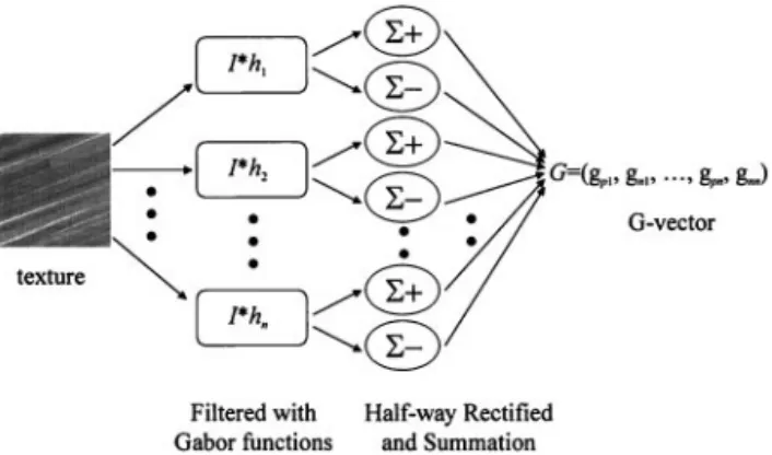
The proposed texture edge detector basically evolves from the texture discrimination model proposed by Chen (1994). In Chen’s study, a psychophysical ex-periment was carried out to quantify the perceptual sim-ilarities between a reference random dot texture and 16 isoperiodicity textures. In parallel to the psychophysical experiment, each texture, denoted as I, was convolved with a bank of filters which were either Gabor or DOOG functions with different orientations and frequencies, as illustrated in Fig. 2 by I*hk, where ‘*’ denotes the 2-D convolution and hkthe kth Gabor function. The integra-tion over the output of a given polarity (on or off), which simulated half-wave rectification of a V1 simple cell, gave a single number representing the response of a filter to a texture. For the filtered image using the kth Gabor function, ⌺⫹ and ⌺⫺ represent the integration opera-tions of the positive and negative pixels, respectively, in Fig. 2. The sum of the positive pixel values and that of the negative pixel values are denoted by gpk and gnk, respectively. For a given texture, this number defined the coordinate of a point along the axis associated with the filter of a given polarity in the N-dimensional space
Fig. 1. The rosette map for the selected set of Gabor filters in frequency domain, in which each Gabor function consists of two Gaussian functions (ellipses) symmetrical with respect to the origin and only the portion larger than the half-peak
mag-nitude is shown for each Gaussian function.
Fig. 2. Derivation of the G-vector, where I*hk stands for convolving the image with the kth Gabor function,⌺⫹ and ⌺⫺ represent the integration operations over the positive and neg-ative pixel values, respectively, and the vector G denotes the
defined by the bank of filters employed. The vector formed by the N numbers (i.e., the vector G in Fig. 2) uniquely defining a point in the N-dimensional space for each texture is called G-vector in this paper for conve-nience. The perceptual similarity between two textures was modeled as the Euclidean distance between their corresponding G-vectors. The results of his study showed that the similarities predicted by this model closely agreed with those obtained by the psychophysical experiments.
Supported by the psychophysical experiments, Chen (1994) not only provides an effective mathematical model to quantify the perceptual similarity between two textures, but also implicitly suggests that a texture may be characterized by its G-vector. Based on Chen’s results and recent physiological findings, the proposed edge detector has been designed to capture the texture edge with a weak RMGD by transforming the G-vectors of local texture information into the distance map and the difference mask that, together, define the desirable edges. More specifically, the proposed edge detection is com-posed of four steps as described in the following.
Step 1: Compute the G-vectors of local textures for each pixel. Unlike Chen’s approach and most previous
early vision models, in which the neuroimages are ob-tained by convolving the entire image with Gabor filters (or other models of receptive field profiles), the proposed approach characterizes the textures surrounding each pixel within a small block. As illustrated in Fig. 3, the underlying image I is decomposed into overlapping blocks of constant size. Suppose the image size is N⫻ N and the block size is M⫻ M. We will have (N ⫺ M)2 blocks, each centered at a pixel in the central (N⫺ M) ⫻ (N ⫺ M) region of the image I. Then, for each block, compute the G-vector with the predefined set of even Gabor filters, which may be formally expressed as fol-lows. Denote the block centered at the pixel (i, j) of the image I as B(i, j) and the G-vector computed from B(i,
j) as G(i, j). Let Bk(i, j) ⫽ B(i, j)*hk and Bpk(i, j) denote the half-way rectified Bk(i, j) of positive polarity [i.e., all negative pixels values are set to zero in the neuroimage, Bk(i, j)]. Also, the value of the pixel (r, s) in Bpk(i, j) is denoted by Bpk(i, j)[r][s]. Similarly,
Bnk(i, j) denotes the half-way rectified Bk(i, j) of neg-ative polarity. Suppose n Gabor filters are used. Define:
G共i, j兲 ⫽ 共 gp1共i, j兲, gn1共i, j兲, . . . ,
gpk共i, j兲, gnk共i, j兲, . . . , gpn共i, j兲, gnn共i, j兲兲 (7) and gpk共i, j兲 ⫽
冘
r⫽1 M冘
s⫽1 M Bpk共i, j兲关r兴关s兴 (8) gnk共i, j兲 ⫽冘
r⫽1 M冘
s⫽1 M Bnk共i, j兲关r兴关s兴, (9)where hk is the kth Gabor function and * the 2-D con-volution.
The size of a block should be selected so that the number of texcels in each block is adequate to represent the speckles and the tissue-related textures. Because, for a US image with a good quality, a block of size 8⫻ 8 or 16⫻ 16 usually comprises a sufficient number of speck-les and texcels, these two block sizes have been em-ployed throughout our studies. Choosing a block size of a power of two is for fast implementation of the 2-D convolution.
Step 2: Compute the distance map. The distance
map, DIST, of the underlying image is defined as
DIST(i, j)⫽ 储G(i, j)储, where 储 x储 is the 2-norm of the
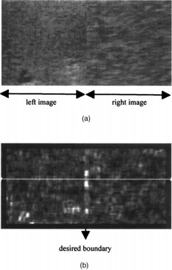
vector x. Then, the peaks in the distance map suggest the edge locations. To demonstrate the distance map, Fig. 4a is used as the source of the texture image, which is a synthetic edge image consisting of two 128⫻ 128 US images. To ensure a weak RMGD around the desired edge, the image intensity of both US images has been adjusted so that the RMGD between the rightmost four columns of the left image and the leftmost four columns of the right image is zero. As a result, Fig. 4b gives the distance map derived by using the block size of 8⫻ 8 for Fig. 4a. The line profile of the 53rd line of the distance map, which is marked by a white line in Fig. 4b, is plotted in Fig. 5. One can see that a peak does exist at the border of two textures in the distance map.
To see what texture features have been exploited by the distance map and why a peak can be formed at the texture boundary, without loss of generality, consider the
Fig. 3. Given the image size N⫻ N and the block size M ⫻ M, decomposing the underlying US image into (N⫺ M)2
blocks, each centered at a pixel in the central (N⫺ M) ⫻ (N ⫺ M)
contribution from one element, say gpk(i, j), in G(i, j) to DIST(i, j). Then, gpk 2共i, j兲 ⫽
冉
冘
r⫽1 M冘
s⫽1 M Bpk共i, j兲关r兴关s兴冊
2 ⫽ Ppk共i, j兲共1 ⫹ Xpk共i, j兲兲 (10) and Ppk共i, j兲 ⫽冘
r⫽1 M冘
s⫽1 M 共Bpk共i, j兲关r兴关s兴兲 2 (11) Xpk共i, j兲 ⫽ 2冘
r1⫽1 M冘
s1⫽1 M冘
r2⫽1 M冘
s2⫽1 M 共r1, s1兲 ⫽ 共r2, s2兲 ⫻冉
Bpk共i, j兲关r1兴关s1兴冑
Ppk共i, j兲 䡠 Bpk共i, j兲关r2兴关s2兴冑
Ppk共i, j兲冊
⫽ M2冢
1⫺ 1 1⫹2冣
, (12)where and 2are the mean and the variance of Bpk(i,
j), which are defined as
⫽r
冘
⫽1 M冘
s⫽1 M Bpk共i, j兲关r兴关s兴 M2 (13) 2⫽Ppk共i, j兲 M2 ⫺ 2 . (14) Equation (10) decomposes gpk 2(i, j) into two mul-tiplicative factors, Ppk(i, j) and Xpk(i, j). Ppk(i, j) is actually the AC power of the half-way rectified neuro-image of positive polarity, Bpk(i, j). Note that the DC power is zero because the DC component has been set to zero for each Gabor function. On the other hand, Xpk(i,
j) measures the uniformity of Bpk(i, j). Generally, the more uniform the Bpk(i, j) is, the smaller the
2
/ will be and, hence, the larger the Xpk(i, j) will be. Therefore, each element of the G-vector is made up of two texture features, namely, the AC power and the uniformity in the corresponding half-way rectified neuroimage of a given polarity.
Because derivation of a distance map involves such nonlinear operations as half-way rectification, square, and so forth, formally showing why a peak can be formed at the texture border is basically a difficult prob-lem. Nevertheless, one may still gain some insight into the behavior of the distance map around the texture border by analyzing the AC power and the uniformity of each element in the G-vector. For ease of analysis, as illustrated in Fig. 6, a bipartite image composed of two texture images with the texture border at the central
Fig. 5. The line profile of the 53rd line of the distance map, which corresponds to the white line marked in Fig. 4b, showing
a peak at the border of two textures.
Fig. 4. (a) A synthetic edge image consisting of two 128⫻ 128 US images. (b) The distance map of the synthetic edge image
column is used for investigating the AC power. Take any block, B(i, j), containing the texture border as an exam-ple. Each block B(i, j) is composed of two textures, namely, the left and the right textures. Suppose the sizes of the block, the left texture and the right texture are M⫻
M, M⫻ (M ⫺ l ) and M ⫻ l, respectively. The total AC
power contained in the distance map of B(i, j) is:
total AC power⫽
冘
k⫽1 n共Ppk共i, j兲 ⫹ Pnk共i, j兲兲, (15) where Pnk(i, j) is the AC power of the half-way rectified neuroimage of negative polarity. According to the Parserval’s theorem, the total AC power may be ex-pressed in the frequency domain as:
total AC power⫽
冘
u⫽1 M冘
v⫽1 M冏
冉
k冘
⫽1 n 共F共hk兲 䡠 F共B共i, j兲兲兲冊
⫻ 关u兴关v兴冏
2 ⫽冘
u⫽1 M冘
v⫽1 M冏
冉冉
k冘
⫽1 n F共hk兲冊
䡠 F共B共i, j兲兲冊
关u兴 ⫻ 关v兴冏
2 ⬇ C冘
u⫽1 M冘
v⫽1 M 兩F共B共i, j兲兲关u兴关v兴兩2 , (16)where C is a constant, F( 䡠 ) the 2-D discrete Fourier transform (2-D DFT) and 兩x兩 is the magnitude of the complex number x. From the second line to the third line in eqn (16), it is assumed that the magnitudes of all frequency components in the sum of all Gabor functions are approximately equal. For example, the ratio of the SD to the mean of all frequency components is less than 10% for the sum of the Gabor functions defined in the rosette map when M ⫽ 64. This ratio may be further reduced if more Gabor functions are used or proper weights are assigned to the Gabor functions.
Roughly speaking, the total AC power captured by the distance map for each block B(i, j) is proportional to the total power of B(i, j). Denote the regional mean grey levels of the left texture, the right texture and the entire
block of B(i, j) as ml, mr, and ma, respectively. It is assumed that both left and right textures are homoge-neous so that ml and mr are independent of the texture areas. Again, using the Parserval’s theorem, the total power of B(i, j) may be expressed as:
1 M2
冘
u⫽1 M冘
v⫽1 M 兩F共B共i, j兲兲关u兴关v兴兩2⫽冘
r⫽1 M冘
s⫽1 M 兩B共i, j兲关r兴关s兴兩2 ⫽冘
r⫽1 M冘
s⫽1 M⫺l 共B共i, j兲关r兴关s兴 ⫺ ml兲 2⫹冘
r⫽1 M冘
s⫽M⫺l⫹1 M 共B共i, j兲 ⫻ 关r兴关s兴 ⫺ mr兲2⫹ M共M ⫺ l 兲共ml⫺ ma兲2 ⫹ Ml共mr⫺ ma兲2⫹ M2ma 2 . (17) Equation (17) divides the total power of B(i, j) into the power purely from textures (i.e., the first two terms), the power from the regional mean grey levels (i.e., the sec-ond two terms) and the power from the DC component (i.e., the last term). Because both left and right textures have been assumed to be homogeneous, each of the first two terms would be linearly proportional to the texture area. Hence, the sum of the first two terms would be a monotonic function of l, for l from 0 to M. For the second two terms, one can easily show that, if mr⫽ ml, the sum of the second two terms is monotonically in-creasing with l, for l from 0 to M/ 2, and monotonically decreasing with l, for l from M/ 2 to M. The maximum of the sum of the second two terms, thus, occurs at l⫽M/ 2. The second two terms diminish if mr ⫽ ml. The last term is actually the DC component of the block B(i,
j) and will be cancelled when filtered with the Gabor
functions because the DC component of all Gabor func-tions have been set to zero. As a result, as a block slides from the left of the texture border to the right, one may expect a local maximum at the texture border for the total power of the block. Because the total AC power con-tained in the distance map is roughly proportional to the total power of each block, a local maximum may be observed at the texture border for the total AC power of the distance map.
Although the decisive information captured by the AC power, Ppk(i, j), is the variation of the low fre-quency information (i.e., the information based on the regional mean grey levels) the major information caught by the uniformity, Xpk(i, j), is the middle- to high-frequency information. Consider a block, B(i, j), in the bipartite image given in Fig. 6, and a middle- to high-frequency Gabor function, hk. Initially, suppose B(i, j) consists of only one texture. Then, because a texture is composed of periodic or quasiperiodic texcels, Bpk(i, j) is also periodic or quasiperiodic and it is very likely that most energy of Bpk(i, j) is concentrated in the periodic or quasiperiodic blobs as a result of filtering with a
middle-Fig. 6. The model of a bipartite image used in the analysis of the total AC power contained in the distance map of each block.
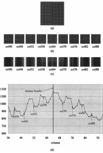
to high-frequency Gabor function. As the block moves from one texture to the other, say, from the left of the texture border to the right, the energy concentration phenomenon will be disturbed when the other texture (the right texture) appears in the block. In other words, more and more energy will start to spread over the entire block as the area of the right texture is getting larger. That is, the2/ of Bpk(i, j) tends to become smaller as the block moves from the left toward the texture border. Likewise, a similar argument may be made for a block moving from the right to the left. By symmetry, it is reasonable to expect a local minimum for the2/ and, hence, a local maximum for the Xpk(i, j) at the texture border. As an example, Fig. 7d demonstrates the change of the uniformity, Xpk(i, j), for a 64⫻ 64 block moving from the 36th column to the 95th column centered at the 64th row in the 128⫻ 128 LM texture image shown in
Fig. 7a. The texture border is at the 64th column. The main reason why an LM texture image rather than a synthetic US edge image is used is that, from a US image, it is relatively difficult to find a homogeneous subimage as large as 128⫻ 128 for extracting blocks of size 64 ⫻ 64, which is considered as the minimal ac-ceptable size for presentation. To better visualize the correlation between the uniformity and the energy dis-tribution (i.e., the grey-level disdis-tribution) over the entire block, B(64, 40⫹ 6t) and Bpk(64, 40 ⫹ 6t), for t ⫽ 1 to 9, are provided in Fig. 7b and c, respectively. The uniformity corresponding to each of these blocks is also marked in Fig. 7d. The central frequency of the Gabor function used is (u0, ) ⫽ (4公2, /3) in the polar
coordinate system. All blocks in Fig. 7c have been quan-tized by the same decision and output levels for visual comparison of relative brightness. One may see from Fig. 7c that the strips in the block marked as “col64” are more uniform and dimmer than those in other blocks, which results in a higher uniformity. Note that the uni-formity variation shown in Fig. 7c and d would be less evident for using a low-frequency Gabor function be-cause the texture information may be smeared too seri-ously to characterize different textures.
In summary, DIST(i, j) comprises two major tex-ture information. One is the total AC power involved in all neuroimages, which is roughly proportional to the total power of the underlying block of image. For a block centered at the texture border, because the areas of both textures are about the same, the total AC power may contribute a local maximum in the distance map, pro-vided that the regional mean grey levels of both textures in the block are different. The other texture information contained in DIST(i, j) is the uniformity measurement in each half-way rectified neuroimage of a polarity. In contrast to the total AC power, which mainly utilizes the low-frequency information (i.e., the regional mean grey levels) to generate a peak at the texture border, the uniformity variation would be more evident for the half-way rectified neuroimage of a polarity computed from a middle- to high-frequency Gabor function. A local max-imum of uniformity may occur at the texture border because the half-way rectified neuroimage of a polarity derived from a block centered at the texture border is usually more uniform in terms of 2/ than the corre-sponding half-way rectified neuroimages from the adja-cent blocks.
Step 3: Compute the difference map and the differ-ence mask. The distance map plays the decisive role in
identifying the potential edges. Nevertheless, the differ-ence mask generated from the differdiffer-ence map further confines the regions where the desired edges might exist to suppress the false peaks due to the noisy nature of the
Fig. 7. Demonstration of uniformity variation across a texture border along the 64th row of a texture image. (a) A 128⫻ 128 LM texture image with the texture border at the 64th column; (b) nine blocks of the original image, including B(64, 40 ⫹ 6t), t ⫽ 1 to 9. (c) Bpk(64, 40 ⫹ 6t), t ⫽ 1 to 9. (d) Uniformity from the 36th column to the 95th column (i.e.,
Xpk(64, j), j ⫽ 36 to 95). The label beneath each block of image is the column number of this block.
US image, as shown in Fig. 5. The difference map,
DIFF, of the underlying image is defined as:
DIFF共i, j兲 ⫽ 共储G共i ⫺ 1, j兲 ⫺ G共i, j兲储2⫹ 储G共i, j ⫺ 1兲
⫺ G共i, j兲储2兲1/ 2
. (18) Recall that G(i, j) is the G-vector of the block B(i, j). Conceptually, the difference map computes the compos-ite perceptual similarity between the horizontal adjacent blocks and vertical adjacent blocks based on Chen’s model (Chen 1994). The difference map of Fig. 4a, derived by using the block size of 8⫻ 8, is provided in Fig. 8a, and the line profile of its 53rd line, which corresponds to the white line marked in Fig. 8a, is plotted in Fig. 9. From Fig. 9, one may observe that the differ-ence map does not generate a significant peak at the texture border. That is, two adjacent blocks are not the most dissimilar at the texture border. In practice, the actual peak position is dependent on the texcel size. As the block moves from the left texture to the right one, ideally DIFF(i, j) remains zero when the block contains only one texture. When the block starts to include the right texture, DIFF(i, j) starts to have a positive value. It is conjectured that DIFF(i, j) reaches a local maxi-mum when the portion of the right texture in the block is just large enough partially to exhibit the right texture property. Suppose, at this time, the center of the block is (i0, j0). It is because, at this time, G(i0, j0⫺ 1) mainly
sees the texture features from the left texture, whereas
G(i0, j0) sees texture features from both of the left and
the right textures. After that, as the block moves toward the texture border, because the areas of both textures in
every two adjacent blocks only differ slightly, the dif-ference of the texture information contained in the G-vectors of every two adjacent blocks is expected to be minor. Hence, it is reasonable to anticipate a DIFF(i, j) smaller than the local maximum, DIFF(i0, j0).
Although the difference map may not be used to pinpoint the desired edges, it does reveal the great pos-sibility to find the desired edges within the regions en-closed by the significant peaks. This observation has led to the design of the difference mask, which serves as a useful mask to suppress the undesired edges suggested by the distance map. The goal is to extract the area enclosed by the local maximums at the left side and the
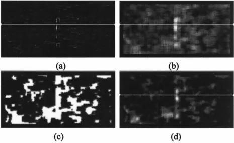
Fig. 8. (a) The difference map of Fig. 4a derived by using the block size of 8⫻ 8. (b) The dilated difference map using grey-level dilation with an 8 ⫻ 8 structuring element; (c) The difference mask; (d) The difference mask weighted
distance map.
Fig. 9. The line profiles of the 53rd lines of the difference map, the dilated difference map and the difference mask weighted distance map, which correspond to the white lines marked in
right side of the texture border in the difference map. To generate the difference mask, a grey-level dilation using an M ⫻ M (i.e., the block size) square structuring element is first applied to the difference map to fill up the regions enclosed by the significant peaks. The grey-level dilation operator GD(I(i, j), Sp), which dilates pixel (i,
j) of image I using the p⫻ p structuring element Sp, is defined as:
GD共I共i, j兲, Sp兲 ⫽ max共Iul兲 ⫹ max共Iur兲 ⫹ max共Ill兲
⫹ max共Ilr兲, (19) where Iul⫽ I共i ⫺ p/ 2: i, j ⫺ p/ 2: j兲 (20) Iur⫽ I共i ⫺ p/ 2: i, j ⫹ 1: j ⫹ p/ 2 ⫺ 1兲 (21) Ill⫽ I共i ⫹ 1: i ⫹ p/ 2 ⫺ 1, j ⫺ p/ 2: j兲 (22) Ilr⫽ I共i ⫹ 1: i ⫹ p/ 2 ⫺ 1, j ⫹ 1: j ⫹ p/ 2 ⫺ 1兲. (23) In words, the grey-level dilation operator GD(I(i, j), Sp) replaces I(i, j) by the sum of the maximums of the four regions defined by Iul, Iur, Ill and Ilr. Following the grey-level dilation, the dilated difference map is thresh-olded by its mean value and set the pixels larger than the threshold to 255, which results in a binary image con-taining 0-pixels and 255-pixels. At this stage, it is ex-pected that the desired edges would be covered by the 255-pixels. However, due to the noise in the difference map, the binary image may contain undesirable small clusters of 255-pixels. Also, the sizes of the 255-pixel clusters covering the desired edges may be unnecessarily large and can be shrunk. Thus, the binary image is eroded by a 3⫻ 3 structuring element and the eroded image is smoothed by a Gaussian function of SD 1, which gives the difference mask. Because the edges of the eroded image are step edges, the smoothing operation is to eliminate the false edges that may be introduced by the step edges when using the eroded image as the mask. Taking Fig. 4a as an example, Fig. 8a– c shows the difference map, dilated difference map and difference mask of Fig. 4a. The line profiles of the 53rd lines, the difference map and the dilated difference map are plotted in Fig. 9, which correspond to the white lines marked in Fig. 8a and b, respectively. From Figs. 8 and 9, one can see that the dilated difference map has succeeded in defining a significant region around the border, and the difference mask has effectively excluded a great amount of undesired area.
Step 4: Compute the difference mask weighted dis-tance map. After the disdis-tance map and difference mask
have been derived, the difference mask weighted dis-tance map, WDIST, may be easily obtained by comput-ing WDIST(i, j) ⫽ DIST(i, j) 䡠 DM(i, j), where DM denotes the difference mask. Finally, the WDIST is smoothed by a Gaussian function and the peaks of the smoothed WDIST define the potential edges. The Gauss-ian function is to reduce the noise in the WDIST. For example, the weighted distance map (Fig. 8d) resulting from the distance map and the difference mask given in Fig. 4b and Fig. 8c, respectively, has greatly reduced the possible areas where the desired peaks in the distance map (Fig. 4b) might exist. The 53rd line profiles of the weighted distance map, labeled as “weighted distance map” in Fig. 9, clearly show that the difference mask has successfully eliminated many undesired false peaks in comparison with the 53rd line profile of the distance map illustrated in Fig. 5. Finally, one may apply a threshold-ing technique to determine the desired edges.
As a summary, the proposed texture edge detector is composed of four steps. In step 1, the image is decom-posed into overlapping blocks and the G-vector, G(i, j), for each block, B(i, j), centered at the pixel (i, j) is computed using the Gabor functions defined in the ro-sette map show in Fig. 1. In step 2, the distance map,
DIST, of the underlying image, which is defined as DIST(i, j) ⫽ 储G(i, j)储 is computed. The peaks in the
distance map suggest the edge locations. In step 3, the difference mask, which is generated from the difference map, to suppress the false peaks in the distance map is computed. The difference map, DIFF, is defined by eqn (18). The difference mask is derived by applying the grey-level dilation operator defined in eqn (19) to the difference map, followed by thresholding, binary erosion and Gaussian smoothing. In step 4, the distance map is masked by the difference mask and the WDIST is smoothed with a Gaussian function. The desired edges are determined from the peaks in the smoothed WDIST, for example, by thresholding techniques.
Texture enhancement
Even with a texture edge detector, false edges may be easily generated due to the sporadic spots and arte-facts in a US image. Obviously, the conventional denois-ing techniques cannot be used because the texture infor-mation may be spoiled greatly by the smoothing opera-tions. To preserve the texture patterns used for identifying the texture edge with a weak RMGD, a new concept of denoising for texture enhancement is pro-posed in this paper. Instead of smoothing the original image, which may destroy the structures of all scales, smoothing operations are only applied to those of
se-lected scales. To achieve this goal, wavelet analysis is employed to extract information of different scales.
Wavelet transform may be viewed as an operation projecting an image onto subspaces of different resolu-tions (scales). Because wavelet bases have a higher com-pact support than sinusoidal functions, wavelet trans-form, in general, provides a much better locality than Fourier transform. Taking 1-D discrete wavelet trans-form (DWT) as an example, mathematically, 1-D DWT up to a level J of depths for a discrete signal x(n), n⑀Z, may be formulated as follows:
x共n兲 ⫽
冘
j⫽1 J冘
k⑀Z dj,kj,k r共n兲 ⫹冘
k⑀Z aJ,kJ,k共n兲, (24) and dj,k⫽冘
n x共n兲j,k共n兲 (25) aJ,k⫽冘
n n x共n兲J,k共n兲, (26) where:(t)⫽continuous scaling function, (t)⫽continuous wavelet function,
r(t)⫽continuous reconstructing wavelet function,
j,k(n)⫽discrete version of the scaling function at scale 2jand position k,
j,k(t) ⫽ 2⫺j/ 2(2⫺j/ 2t ⫺ k),
j,k(n)⫽discrete version of the wavelet function at scale 2jand position k,
j,k(t)⫽ 2⫺j/ 2(2⫺j/ 2t ⫺ k),
j,kr (n)⫽discrete version of the reconstructing wavelet function at scale 2jand position k,
j,k r (t) ⫽ 2⫺j/ 2r(2⫺j/ 2t ⫺ k),
dj,k⫽detail coefficients at scale 2jand position k,
aJ,k⫽approximation coefficients at scale 2Jand position k.
By using 1-D DWT, for a J levels of decomposition, a discrete signal x(n) may be decomposed into J levels of detail signals (i.e., the detail signals from level 1 to level J) and an approximation signal at level J. The detail signal at level j, denoted as Dj( x(n)), may be computed from dj,k by Dj( x(n)) ⫽ ¥k dj,kj,k
r
(n) and the approximation signal at level J, denoted as AJ( x(n)), may be derived from aJ,kby AJ( x(n))⫽ ¥kaJ,kJ,k(n). The approximation signal at level i, Ai( x(n)), represents the approximated (smoothed) version of the original sig-nal x(n) with a resolution of one point for every 2ipoints of the original signal. The detail signal at level i,
Di( x(n)), stands for the difference in information be-tween the approximated versions of the original signal
x(n) at two successive resolutions. As a matter of fact,
the following iterative relation holds for the detail and approximation signals at two successive levels, where
A0( x(n)) ⫽ x(n):
Ai⫺1共 x共n兲兲 ⫽ Ai共 x共n兲兲 ⫹ Di共 x共n兲兲. (27) Similarly, for the 2-D DWT, an image may be decomposed into four images (i.e., one approximation and three details) at each level of resolution. These three details are horizontal, vertical and diagonal details.
To preserve the texture information as much as possible in the texture enhancement process, our idea to minimize the influence of the false edges is to perform smoothing operation (e.g., using a Gaussian filter) on the approximation at level J (i.e., A) rather than on the original image. This idea has inherently assumed that the small-scale texture information is mainly comprised in the details at the first J levels. Note that J is image-dependent and strongly related to the scales of the struc-tures to be smoothed. After smoothing, the denoised image, Id, may be reconstructed from the details in the first J levels and the smoothed AJ, denoted as SAJusing a relation similar to eqn (27) for 2-D DWT as follows:
Id⫽
冘
i⫽1J
共Hi⫹ Vi⫹ Di兲 ⫹ SAJ. (28) For US images, a reasonable choice of J is J⫽ log2M,
where M ⫻ M is the block size for computation of the distance map. The rationale of this choice is as follows. Because, in theory, an M ⫻ M block would extract the texture information with texcels not larger than M/ 2⫻
M/ 2 according to the Nyquist rate, the structures larger
than M/ 2 ⫻ M/ 2 hardly contribute valuable texture information to the distance map. On the other hand, because the equivalent resolution in AJ is about 2
J , smoothing AJ should not ruin any useful texture infor-mation that might be used in the distance map. This texture-enhancement idea can be further generalized to multiresolution filtering, if necessary. In other words, one may apply Gaussian filters of different SDs to the different levels of approximations.
Performance analysis
Two types of US images have been employed to evaluate the performance of the proposed edge-detection algorithm. One is the synthetic edge image and the other is the clinical US image. The synthetic edge image is a composite bipartite image consisting of two 128⫻ 128 US images, as shown in Fig. 4a. Because the border of
two textures is well defined, the synthetic edge image serves for the exact performance evaluation of the pro-posed algorithm. On the other hand, the detected edges of the clinical US images are compared with the bound-aries manually drawn by an experienced medical doctor. Because the edges in the clinical US images usually are not well defined, delineating the boundaries of the ob-jects of interest is quite a subjective process. As a result, the manually delineated boundary of an object frequently varies substantially with that of the medical doctor. Therefore, it should be emphasized that this performance evaluation can only serve as a reference.
Because the focus of this paper is on those texture edges with a weak RMGD, for comparative study, the proposed algorithm has been compared to two nontex-tural edge detectors and two texnontex-tural edge detectors using the synthetic edge images. The nontextural edge detec-tors are taken into account because most previous ap-proaches are nontextural apap-proaches and the texture edges still have detectable RMGD, though weak, that can certainly be utilized by the nontextural approaches. The comparison with the nontextural edge detectors is in-tended to show the important role of the texture infor-mation, even when the RMGD is relatively strong.
The two nontextural edge detectors are the Laplacian-of-Gaussian (LOG) (Marr and Hildreth 1980) and the Canny edge detectors (Canny 1986). The LOG is a widely used edge detector that defines the edges at the zero-cross-ing points of the second derivative of the Gaussian-smoothed image. The LOG usually achieves a much better performance than many other classic approaches, especially in cases of low signal-to-noise ratio (Parker 1997). The Canny edge detector is an optimal operator with respect to a set of criteria (i.e., good detection, good localization, and single response). Even though these two nontextural edge detectors have been designed with a smoother, their perfor-mance on US images is usually unacceptable due to the speckles and tissue-related textures. To ensure the fairness of the comparison among different algorithms, the under-lying principle in the experimental design was to maximize the intended capability of each algorithm. Therefore, for the LOG and the Canny operators, the speckle reduction algo-rithm proposed by Karaman et al. (1995) has been carried out on the synthetic edge images before these two edge detectors were applied. The reason why a speckle-reduction algorithm rather than a denoising method is employed is that the former can usually preserve the object boundary better than the latter, by taking into account the statistical property of the speckles. In this study, we have employed the LOG and the Canny edge detectors provided in the commercial software tool, MATLAB.
The two textural edge detectors are the early vision model-based approaches proposed by Jain and Farrokh-nia (1991) and Malik and Perona (1990). In the approach
of (Jain and Farrokhnia 1991), each texture image is filtered with a set of even Gabor functions forming a rosette map in the frequency domain. Among all filtered images, the significant filtered images are selected so that the summed power is 95% of the total power. Following selection of the significant filtered images, a nonlinear hyperbolic transform is applied to each filtered image and the transformed image is averaged with a weighting window (e.g., a Gaussian function) to measure the local energy. The energy maps derived from all selected fil-tered images form a feature vector for each pixel. A clustering algorithm called CLUSTER is employed to find the texture boundary, which recursively assigns each pixel to the cluster with the shortest Euclidean distance between the feature vector of the pixel and that of the centroid of the cluster.
In the algorithm of (Malik and Perona 1990), each texture image is convolved with a set of filters (DOG and DOOG) followed by half-way rectification. Two DOG functions have been used, namely DOG1 and DOG2, which are defined as:
DOG1共兲 ⫽ a 䡠 G共0, 0, i,i兲
⫹ b 䡠 G共0, 0,0,0兲 (29)
DOG2共兲 ⫽ a 䡠 G共0, 0, i,i兲 ⫹ b 䡠 G共0, 0,, 兲
⫹ c 䡠 G共0, 0, 0,0兲, (30)
where G( x0, y0, x, y) is the Gaussian function, as defined previously. For DOG1,i: : 0is 0.71:1:1.14
and a:b is 1:⫺1. For DOG2,i:: 0is 0.62:1:1.6 and
a:b:c is 1:⫺2:1. An inhibition scheme is then applied to
suppress the weak response based on the so-called postinhibition response (PIR). The PIR selects the stron-gest thresholded and weighted response from the sam-pling neighborhood of each pixel in each channel. The threshold for each pixel in each channel is the maximal weighted response in the neighborhood of the pixel de-fined over all channels. The weighting factors are related to the measure of the effectiveness of inhibition. The texture boundaries are defined by the local peaks in the texture gradient, which is the maximum of the gradient of the PIR smoothed by a Gaussian function among all channels for each pixel.
The performance of each edge detector is evaluated using the figure suggested by Pratt (1980), which is defined as: E⫽ 1 E0max共If, I0兲
冘
i⫽1 If冉
1 1⫹ adi 2冊
, (31) whereIf⫽the number of edge pixels found by the edge detector,
Io⫽the actual number of edge pixels,
di⫽the shortest distance from the ith detected edge pixel to the ideal boundary,
a⫽the scaling factor, which is set to 1 in our
analysis,
Eo⫽the normalization factor to take into account the discrete nature of a digital image.
The reason for using the Pratt’s figure as the performance index is that it not only measures the distance between the all detected edges and the corresponding desired edges, but also gives penalty to the excessive number of edge points. For the synthetic edge image, the ideal boundary is an imaginary line at the middle of the 128th and the 129th columns. Therefore, the best performance that an algorithm can achieve is 0.8. In this case, E0is set
to 0.8. For the clinical US image, because the ideal boundary is manually drawn by an experienced medical doctor, there is no discrete problem and E0is set to 1.
IMPLEMENTATIONS AND DISCUSSIONS All US images, including those used to make the synthetic edge images, are selected by medical doctors and captured from a Toshiba SSA-380A clinical US imaging system through a frame-grabber card. The frame-grabber card was the Meteor-II card made by the Matrox Electronic System Ltd., which captured the im-age from the RGB output of the Toshiba SSA-380A and stored the image in the BMP format with 8-bit resolution for each color channel. The operating frequency of the ultrasound system was 3 MHz.
For both of the synthetic edge images and the clin-ical US images, the block size used in the proposed texture edge detector is 8⫻ 8. Accordingly, the decom-position level J for the texture enhancement is log28⫽
3 as discussed above.
Rather than evaluating the performance using the entire image, for each synthetic edge image, the Pratt’s figure has been computed within a performance window, that is defined as the central 80⫻ w pixels (i.e., 80 rows by w/ 2 columns at both sides of the imaginary bound-ary). The reasons are two-fold. One is that it is quite common to perform edge detection within a region-of-interest (ROI). In this case, it is more appropriate to measure the performance of the ROI instead of the entire image. The other is that, since it is not easy to find a large homogeneous area in an clinical US image to make the synthetic edge images, computing the Pratt’s figure in a large region might include edges from other tissues, which are not necessarily false edges. On the other hand, evaluating the performance within a small region may
not be applicable to the practical situations. Therefore, in this paper, five different w s (i.e., w⫽ 20, 40, 60, 80, and 100) have been considered to account for the possi-ble influence of the complex nature of a US image. For succinctness, we will present the performances evaluated using the five different performance windows only for the proposed algorithm. The performance comparison between different algorithms will be made by using one small performance window (w ⫽ 20) and one large performance window (w ⫽ 80), to avoid the possible bias due to the window size. For each clinical US image, the performance is evaluated only for those detected edge points that are less than 10 pixels away from the manually delineated boundary in terms of the Euclidean distance. The size of the performance window is mainly limited by the smallest size of the testing objects of interest and by the criterion imposed by us (i.e., using approximately the same area for inside and outside the boundary in computing the Pratt’s figure).
Because the performance of each edge-detection algorithm is quite dependent on the parameter values used for each image, to avoid an unfair comparison due to an improper selection of the parameter values, we have adopted the best performance attainable in the per-formance comparison. The best parameter values for each algorithm have been sought by a coarse search followed by a fine search. The coarse search is to narrow down the possible ranges of the best parameter values for each image by using a relatively large step size for each parameter. The fine search is to find the best parameter values with a small step size within the range determined by the coarse search. For the LOG and the Canny edge detectors, the best performance was found by varying the only two parameters (i.e., the thresholds and the SDs) specified in the MATLAB commands. For the Jain and Farrokhnia and Malik and Perona approaches, the best performance was derived by using the parameter values given in their papers. In addition, because Malik did not give the values for the radius of the sampling neighbor-hood and the SD of the Gaussian function in computing the texture gradients, coarse and fine searches have been applied to these two parameters to find the best perfor-mance. For the proposed algorithm, the threshold is defined as the mean plus the SD multiplied by a factor,
Tm, where the mean and the SD are calculated over the entire image. The coarse and fine searches have been applied to the SD of the Gaussian function smoothing the
WDIST and the factor Tm. Table 1 summarizes the parameters to which the fine search has been applied as well as their ranges and step sizes used in the fine search for each algorithm. For the Jain and Farrokhnia (1991) algorithm, no fine search has been conducted because the parameter values given in the paper have been employed.
On the synthetic edge images
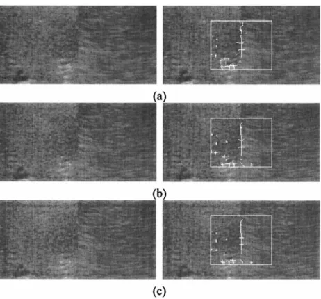
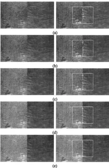
To investigate the effect of the RMGD on the edge-detection performance, 20 sets of synthetic edge images have been employed for performance evaluation and comparison. Each set consisted of five images that were made of the same two 128⫻ 128 US images, but with different RMGDs. For each set, the RMGDs were set to 0, 10, 20, 30 and 40. The RMGD of each synthetic edge image was ensured by adjusting the regional mean grey levels of its two 128⫻ 128 US images so that the RMGD between the rightmost four columns of the left image and the leftmost four columns of the right image met the specified value. As an example, by using the proposed texture edge detector without texture enhancement, Fig. 10 demonstrates the 15th set of the synthetic edge images and the detected edges with the best performance in terms of the Pratt’s figure. In Fig. 10, the RMGDs of the five synthetic edge images are 0, 10, 20, 30 and 40 from top to bottom. The synthetic edge images are in the left column and the corresponding detected edge images are in the right column, side by side. The white rectangle in each right image of Fig. 10 indicates the performance window of size 80⫻ 100.
Without texture enhancement, the best perfor-mances of the proposed edge detector for the 20 sets of synthetic edge images are plotted in Fig. 11 for five different performance windows. In Fig. 11, the vertical axis gives the Pratt’s figure and the horizontal axis ar-ranges data into five clusters, in terms of the RMGD, that are separated by vertical dashed lines. A cluster contains the performance statistics of five groups, each consisting of 20 synthetic edge images with the same RMGD and the same size of the performance window. For conve-nience, the notation convention X[w] will be used to denote the performance of the algorithm X computed with the performance window of size 80 ⫻ w. For the proposed textural approaches, X can be “TED,” “ETED3” and “ETED5,” which stand for the proposed texture edge detector without texture enhancement, with texture enhancement smoothed by a Gaussian function of SD 3, and with texture enhancement smoothed by a
Gaussian function of SD 5, respectively. For the conven-tional algorithms, X can be “LOG,” “Canny,” “Malik,” and “Jain,” which represent the LOG, the Canny, the Malik and Perona, and the Jain and Farrokhnia algo-rithms, respectively.
Due to the skewed distribution of the Pratt’s figures in each group, the quartile statistics (Vardeman 1994) instead of mean and variance has been adopted to de-scribe the performance statistics. For each group in Fig. 11 (i.e., given an RMGD and a performance window) the Pratt’s figures of the 20 synthetic edge images are first sorted in the ascending order. Each vertical rectangular bar corresponds to the median (i.e., the 11th Pratt’s figure) of the sorted sequence, which stands for the averaging performance that the underlying algorithm may achieve for this group. The upper and lower error bars indicate the 15th and the 6th Pratt’s figures in the sorted sequence, which are statistically equivalent to the
Table 1. The parameters and their ranges and step sizes used in the fine search of the best performance for each algorithm
Algorithms Parameters Range Step size Proposed approach Tm ⫺1.5–2.5 0.1 SD 1–3 1 LOG Threshold 0.001–0.01 0.001 SD 0.1–3.0 0.1 Canny Threshold 0.01–0.1 0.01 SD 0.1–3.0 0.1
Malik and Perona Neighborhood radius 2–8 1
SD 4–16 1
Jain and Farrokhnia none NA NA
Fig. 10. The 15th set of synthetic edge images (left column) and the corresponding detected edges (right column) with the best performance computed within the central 80⫻ 100 region: The RMGD of each image is (a) RMGD⫽ 0; (b) RMGD ⫽ 10; (c)
first and the third quartiles of the distribution. The length of the error bar is statistically called the interquartile range, which characterizes the spread of the middle half of the distribution.
Generally speaking, Fig. 11 shows that the proposed edge detector without texture enhancement provides a reasonably high performance, even for a synthetic edge image with a small RMGD. As the RMGD increases, the median performance monotonically increases and the interquartile range monotonically decreases, which means that the proposed scheme promises a more reli-able performance for a larger RMGD. It is because, as the RMGD increases, the second two terms in eqn (17) increase. These two terms basically represent the power due to the difference of the mean grey level of the block and that of each texture. It implies a larger total power for a block containing the texture border and, hence, a large value in the distance map. Consequently, as the RMGD increases, the peaks of the false edges become less significant and, hence, the false edges may be greatly reduced due to the stronger local maxima contributed from the texture border. As the size of the performance window increases, the performance generally decreases, mainly caused by the increased false edges and tissue edges included in the larger area. However, this phenom-enon becomes less evident as the RMGD increases be-cause of the stronger local maxima resulting from the texture border. From Fig. 10, one may see that fewer false edges have been produced and the detected edges are more coincident with the texture border as the RMGD increases.
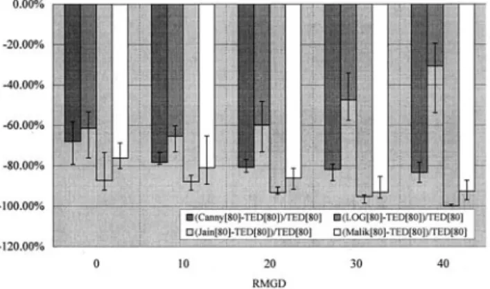
To see the effect of the texture enhancement, like Fig. 11, the relative performance of the proposed algo-rithms, that is (ETED3[w]-TED[w])/TED[w] and (ETED5[w]-TED[w])/TED[w], are plotted in Figs. 12 and 13, respectively, for five sizes of performance win-dows. The vertical axes give the percentages of improve-ment attained by using the texture enhanceimprove-ment. From
Figs. 12 and 13, it is clear that using the texture enhance-ment may achieve a substantial improveenhance-ment over those implementations without using the texture enhancement, though it may also degrade the performance. The im-provement basically increases as the RMGD decreases, due to the more and more important role that the texture information plays in texture edge detection. For a small RMGD (e.g., less than 30) the improvement computed using a large window tends to be better than that using a small window. Moreover, the ETED5[w] is generally better than the ETED3[w], except when w⫽ 20, given a small RMGD. The reason is that a larger smoother (i.e., a Gaussian with a larger SD) may eliminate more false edges than a smaller smoother as intended by the texture enhancement. This effect becomes more obvious in a performance window larger than w ⫽ 20. However, it ought to be noted that the SD of the Gaussian function used in the texture enhancement should not be too large because the edge information due to the RMGD will also be weakened when the false edges are being smeared out.
Fig. 11. The best performances of the TED[w], w ⫽ 20, 40, 60, 80 and 100, for the 20 sets of synthetic edge images.
Fig. 12. The relative performance of the ETED3[w] to the TED[w] (i.e., (ETED3[w]-TED[w])/TED[w], w ⫽ 20, 40, 60, 80 and 100) for the 20 sets of synthetic edge images.
Fig. 13. The relative performance of the ETED5[w] to the TED[w] (i.e., (ETED5[w]-TED[w])/TED[w], w ⫽ 20, 40, 60, 80 and 100) for the 20 sets of synthetic edge images.
Empirically, one may expect a reasonable improvement by using a Gaussian function of SD 3 to 5 for the texture enhancement.
Take the left image in Fig. 10a as an example, which is the original synthetic edge image in the 15th set with the RMGD ⫽ 0. Figure 14b and c shows the texture-enhanced images in the left column and the de-tected edges with the best performance in the right col-umn by using the ETED3 and the ETED5, respectively. The size of the performance window is 80⫻ 100. Figure 10a, which contains the original synthetic edge image and the detected edges, is repeated in Fig. 14a for ease of comparison. It is clear from Fig. 14 that the texture enhancement not only improves the edges around the texture border, but also reduces the false edges.
In performance comparison, because the relative performance among the TED, the ETED3, and the ETED5 algorithms have been presented above, without loss of generality, the TED algorithm has been chosen to represent the proposed algorithms in comparison with the classic approaches. Two sizes of performance win-dows have been considered to avoid the possible bias due to the window size. One is a small performance window (i.e., w ⫽ 20) and the other is a large performance
window (i.e., w ⫽ 80). Figures 15 and 16 give the relative performances between each classic approach and the proposed TED algorithm computed by using the small and the large performance windows, respectively. From Figs. 15 and 16, it is apparent that the TED algorithm outperforms all of the four classic approaches. Moreover, the performance improvement over the classic
Fig. 14. (a) Left: the original synthetic edge image in the 15th set with the RMGD⫽ 0, which is the same as Fig. 10a; right: the edges detected derived by the TED[100] algorithm. (b) Left: the texture-enhanced synthetic edge image using a Gaussian function of SD 3; right: the edges detected derived by the ETED3[100] algorithm. (c) Left: the texture-enhanced synthetic edge image using a Gaussian function of SD 5; right: the edges detected derived by the ETED5[100]
algorithm.
Fig. 15. The relative performance between the classic ap-proaches and the TED algorithm for a small performance
approaches is more significant for a large performance window. Because the texture enhancement also has a better performance in a large performance window, it is expected that the ETED3 and ETED5 may attain a much more significant improvement over the classic ap-proaches. Note that all the vertical rectangular bars are plotted in the negative direction. Although the Jain and Farrokhnia and the Malik and Perona algorithms were designed to detect the texture edges, they perform poorly in US image edge detection probably because of their global approaches to extracting the texture information in the frequency domain. When the two textures forming the texture edge do not generate a prominent frequency pattern in the spectrum of the entire image, it is very likely that the global approaches cannot capture enough texture information to determine the texture edge.
When the performance window is small, the LOG and the Canny edge detectors perform reasonably well for a relatively large RMGD. It is because the speckle reduction process has largely removed the interference of the speckles and the tissue-related textures, while pre-serving the grey-scale edges due to the relatively large RMGD. In addition, one may find that the Canny algo-rithm is slightly better than the LOG algoalgo-rithm. How-ever, when the performance window is large, the relative performance of the Canny algorithm to the TED algo-rithm degrades rapidly, even for those images with a large RMGD. In contrast, although the relative perfor-mance of the LOG algorithm to the TED algorithm also degrades for a large window, the LOG algorithm is much better than the Canny algorithm when the RMGD is large. These results partially support that a nontextural approach may still be useful in US edge detection, as long as the RMGD is large enough.
On the clinical ultrasound images
To evaluate the performance of the proposed algo-rithm in detecting the real boundaries, 20 clinical US
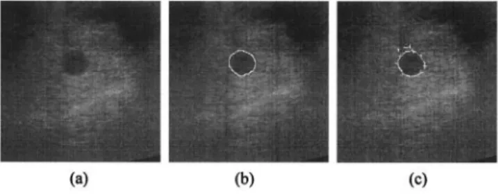
images have been used in this study. The objects of interest are hepatic tumors, such as hepatocellular carci-noma (HCC), cavernous hemangiomas, metastatic liver cancer, hyperplastic nodule, and so on. Limited by the tumor size, the performance on each US image is eval-uated only for those detected edge points that are less than 10 pixels away from the manually delineated boundary in terms of the Euclidean distance. The bound-aries are drawn by an experienced medical doctor by using a self-developed image-processing software called MediaX, which allows a user to make delineation using a mouse or a tablet system. The tablet system used in this study is the Intuos 6 ⫻ 8 tablet (GD0608) made by WACOM company. The RMGDs of the 20 tested tumors are the difference of the mean grey levels between the pixels outside and inside the tumor satisfying the 10-pixel constraint. The RMGDs of the 20 tumors range from 7.8 to 48.5. As examples, Figs. 17–20 show the detected edges for the tumors in images 4, 7, 11 and 20, the RMGDs of which are 17.2, 19.5, 26.2, and 48.5, respectively. In each figure, the left image is the original image, the middle one gives the manually drawn bound-ary, and the right one shows the derived edges.
The best performances of the proposed algorithm on
Fig. 16. The relative performance between the classic ap-proaches and the TED algorithm for a large performance
win-dow (i.e., w ⫽ 80).
Fig. 17. RMGD⫽ 17.2, Pratt’s figure ⫽ 0.338. (a) The original image 4; (b) The manually drawn boundary; (c) The edges detected by the proposed approach. The contrast and brightness of these three images have been linearly adjusted in the same
way for better visualization.
Fig. 18. RMGD⫽ 19.5, Pratt’s figure ⫽ 0.380. (a) The original image 7. (b) The manually drawn boundary. (c) The edges detected by the proposed approach. The contrast and brightness of these three images have been linearly adjusted in the same
![Fig. 12. The relative performance of the ETED3[w] to the TED[w] (i.e., (ETED3[w]-TED[w])/TED[w], w ⫽ 20, 40, 60, 80 and 100) for the 20 sets of synthetic edge images.](https://thumb-ap.123doks.com/thumbv2/9libinfo/8758231.207533/15.918.101.462.109.321/fig-relative-performance-eted-eted-ted-synthetic-images.webp)