超橢圓曲線密碼攻擊之研究

(1)

國

立

交

通

大

學

資訊科學與工程研究所

碩

士

論

文

超橢圓曲線密碼攻擊之研究

A Study on Index Calculus Algorithms

for Hyperelliptic Curves

研究生：林家瑋

指導教授：陳榮傑博士

(2)

超橢圓曲線密碼攻擊之研究

A Study on Index Calculus Algorithms

for Hyperelliptic Curves

研究生：林家瑋 Student：Chia-Wei Lin

指導教授：陳榮傑博士 Advisor：Dr. Rong-Jaye Chen

國立交通大學

資訊科學與工程研究所

碩士論文

A Thesis

Submitted to Institute of Computer Science and Engineering College of Computer Science

National Chiao Tung University in partial Fulfillment of the Requirements

for the Degree of Master

in

Computer Science

June 2007

Hsinchu, Taiwan, Republic of China

(3)

超

橢

圓

曲

線

密

碼

攻

擊

之

研

究

學生：林家瑋

指導教授：陳榮傑博士

國立交通大學資訊科學與工程學研究所碩士班

摘要

1989 年 Koblitz 利用定義在有限域的超橢圓曲線上的 Jacobian 加法群，基於超橢圓曲線離散對數問題的困難度，提出了超橢圓曲線密碼系統。在含有q 個元素的有限域 Fq中，虧格 (genus)為 g 的超橢圓曲線，其中形成離散對數問題的加法群大小為 ( )g O q ，大於橢圓曲線加法群O q 。而且小虧格的超橢圓曲線亦無時間複雜度為次指數的攻擊法，因此適當的設定超橢( ) 圓曲線密碼系統將可使用比橢圓曲線密碼系統更短的密鑰，來達到相同的安全度。目前index calculus 攻擊法在虧格 g 足夠大時，呈現次指數的時間複雜度。當虧格不大時，一般的生日攻擊法為 ₍ 2₎ g O q ，而一般的index calculus 為 _{( )}2

O q 。Thériault 的 index calculus 演算

法加入”大質數”的概念，時間複雜度降為 4 2 2 1 ( g ) O q − − _；而_{Gaudry 等人利用兩個”大質數”的 index} calculus 攻擊法變形，則時間複雜度更進一步改進為 2 2 ( g) O q − 。本文將針對小虧格的超橢圓曲線離散對數問題，實作並改進index calculus 攻擊法。我們亦提出一個更快的演算法來解虧格為2 的超橢圓曲線離散對數問題，其時間複雜度為 O(q)。關鍵字: 超橢圓曲線密碼系統、超橢圓曲線離散對數問題、index calculus

(4)

A St u d y o n I n d e x C a l c u l u s A l g o r i t h m s f o r H y p e r e l l i p t i c C u r v e s

Student：Chia-Wei Lin

Advisors：Dr. Rong-Jaye Chen

Institute of Computer Science and Engineering

College of Computer Science

National Chiao Tung University

ABSTRACT

In 1989, Koblitz proposed using the Jacobian of a hyperelliptic curve defined over a finite field to implement discrete logarithm cryptographic protocols. The discrete logarithm problem of the Jacobian is called hyperelliptic curve discrete logarithm problem (HCDLP). For a hyperelliptic curve of genus g over the finite field Fq, the group order of the Jacobian is O q( )g which is larger

than that of the additive group ,which is O q , in an elliptic curve over F( ) q. Since there is no

subexponential algorithm to solve HCDLP of small genus, hyperelliptic curve cryptosystem under applicable setting requires shorter key size than elliptic curve cryptosystem to achieve the same security level.

When genus g is large enough, the index calculus attack has subexponential time complexity. For small genus HCDLP, the algorithms based on birthday paradox is of time complexity ₍ 2₎

g

O q ,

and the basic index calculus attack is _{( )}2

O q . Thériault improves it by using the large prime

method, and get a running time of

4 2 2 1 ( g ) O q −

− _{. Furthermore, Gaudry et al use a double large prime}

variation for small genus hyperelliptic index calculus, and the time complexity is

2 2 ( g) O q − . In this thesis, we focus on the hyperelliptic curve discrete logarithm problem of small genus, implement and improve index calculus and its variations. We propose a faster algorithm for solving genus 2

(5)

致謝

首先誠摯的感謝指導教授陳榮傑教授，老師悉心的教導使我得以一窺超橢圓曲線密碼學的深奧，不時的討論並指點我正確的方向，使我在求學期間獲益匪淺，也讓這篇碩士論文能夠順利完成。也謝謝洪國寶教授、張仁俊教授、胡鈞祥博士擔任我的口試委員，在口試中給予的指正與建議，使得論文能更加完整。感謝師母李惠慈女士給予我英文寫作上的建議，使論文能更流暢通順。感謝實驗室的志賢學長，及學弟妹們：輔國、用翔、佩娟，謝謝你們的陪伴使我的研究生活更加充實，還有準備口試期間的幫忙，使我能夠更充分準備。最後我也要謝謝我的家人，感謝父母在求學期間多年來的栽培，謝謝弟弟和阿姨不時的關心，有你們的支持使我能夠無後顧之憂的專心求學、完成論文，謹以此文獻給我摯愛的家人。

(6)

List of Figures

Figure 2.1 An elliptic curve C and rational function L1 over ...14

(9)

List of Tables

Table 1.1 NIST Guidelines for Public-Key Sizes with Equivalent

Security Levels ...2

Table 4.1 Time complexity of algorithms solving HCDLP ...28

Table 4.2 Running time (seconds) of hyperelliptic index calculus ...47

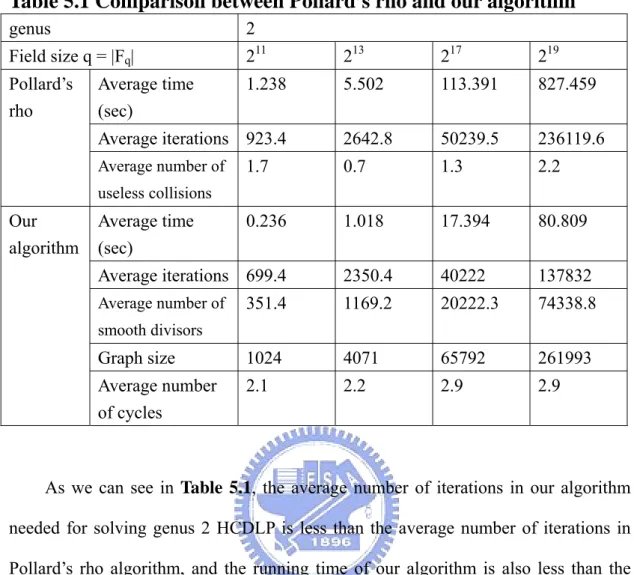
Table 5.1 Comparison between Pollard’s rho and our algorithm ...56

(10)

Notation

The following notation is used throughout this thesis.

K finite

field

K

algebraic closure of a finite field K

F

q

finite field of size q = p

m

for some prime p

q

size of the finite field F

q

g

genus of a hyperelliptic curve

D

0

group of divisors on hyperelliptic curve of degree zero

P

group of principal divisors

J

quotient group J=D

0

/P

div(a,b)

a divisor denoted by Mumford representation with two

polynomials a, b

(11)

Chapter 1 Introduction

1.1 History

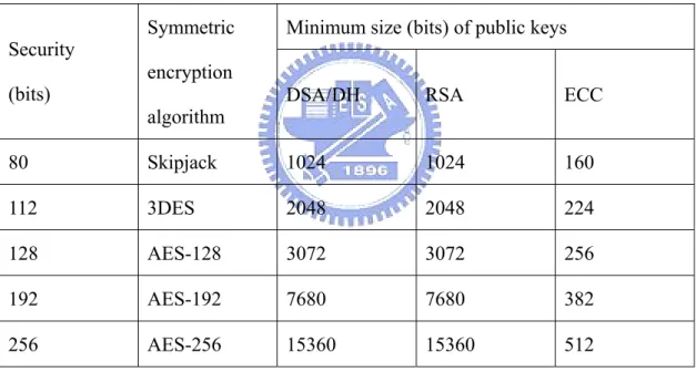
Since the public-key cryptosystems have been invented in 1970s, there are several important public-key cryptosystems of which the security is based on the intractability of discrete logarithm problem (DLP) over a finite abelian group. Elliptic curve cryptography (ECC) [19] is an approach to public-key cryptography based on the algebraic structure of elliptic curves over finite fields. The use of elliptic curves in cryptography was suggested independently by Neal Koblitz and Victor S. Miller in 1985. There is no sub-exponential time algorithm to solve elliptic curve DLP (ECDLP), hence the main advantage of ECC is its smaller key size. A 160-bit key in ECC is considered to be as secure as 1024-key in RSA. As we can see in Table 1.1, ECC key size is much smaller than those of other public-key cryptosystems. Therefore ECC can be implemented efficiently and securely with smaller key size, and is ideally suitable for resource-constrained environments such as smart cards, cell phones, and PDAs.

However, hyperelliptic curve cryptosystems offer even smaller key size. In 1989, Koblitz [20] proposed using the Jacobian of a hyperelliptic curve defined over a finite field to implement discrete logarithm cryptographic protocols. Hyperelliptic curves are a special class of algebraic curves and can be viewed as generalizations of elliptic curves. There are hyperelliptic curves of every genus g ≧ 1. A hyperelliptic curve of genus g = 1 is an elliptic curve. There is no known

(12)

subexponential algorithm for hyperelliptic curves of small genus, and the Jacobian of a hyperelliptic curve of genus g defined over a finite field Fq has group order O(qg).

Hence, the advantage of hyperelliptic curves over elliptic curves is that a smaller base field can be used in order to obtain the same level of security. This makes hyperelliptic curves suitable when only limited memory and computing power is available. Hyperelliptic curves are also of interest because in 2000, Gaudry, Hess and Smart [15] proposed an algorithm which reduces ECDLP over F , for special ₂m values of n, to the hyperelliptic curve DLP (HCDLP) over an sub field of F . ₂m

Table 1.1 NIST Guidelines for Public-Key Sizes with Equivalent Security Levels

Minimum size (bits) of public keys Security

(bits)

Symmetric encryption

algorithm DSA/DH RSA ECC

80 Skipjack 1024 1024 160 112 3DES 2048 2048 224 128 AES-128 3072 3072 256 192 AES-192 7680 7680 382 256 AES-256 15360 15360 512

1.2 The organization of the thesis

The rest of this thesis is organized as follows.

In Chapter 2, we first review some important background in algebra, and introduce algebraic geometry including variety, algebraic curves, and so on. We also

(13)

elliptic curves [24]. The group on a hyperelliptic curve is also based on the divisors. In Chapter 3, we define the hyperelliptic curves over a finite field and the additive group Jacobian associated with a hyperelliptic curve. After defining Jacobian group, we describe the Mumford representation which is used in Cantor’s algorithm to compute the group operation.

In Chapter 4, we describe the index calculus algorithm to solve hyperelliptic curve discrete logarithm problems and several improvements in recent years including the ideas of reduced factor base and large primes. The double large prime variation of hyperelliptic curve index calculus is better than others, and even better than Pollard’s rho method when the genus of the hyperelliptic curve is larger than 2.

In the case of genus 2 curves, Pollard’s rho algorithm is faster than index calculus algorithm. In Chapter 5, we propose an algorithm for solving genus 2 HCDLP which has the same time complexity as Pollard’s rho method. Several computational comparisons are given in section 5.4 to shows that our algorithm is faster than Pollard’s rho method in practice.

(14)

Chapter 2 Mathematical Background

This chapter introduces some elementary mathematical background used in this thesis, including definitions and theorems in abstract algebra and algebraic geometry. If the readers are interested in more of the background, [10] and [11] give good introductions. In section 2.3, we introduce the divisor theory which is the basis of hyperelliptic curve group law. For more details on divisor theory, the reader is referred to [24][25].

2.1 Abstract algebra

Definition 2.1 (Group)

A group (G, *) is a set G with a binary operation * that satisfies the following four axioms:

¾ Closure: For all a, b in G, the result of a * b is also in G. ¾ Associativity: For all a, b and c in G, (a * b) * c = a * (b * c).

¾ Identity element: There exists an element e in G such that for all a in G, e*a= a*e= a.

¾ Inverse element: For each a in G, there exists an element b in G such that a* b= b* a = e, where e is an identity element.

(15)

Definition 2.2 (Abelian group)

A group G is said to be an abelian group (or commutative) if the operation is commutative, that is, for all a, b in G, a * b = b * a.

Definition 2.3 (Cyclic group)

A cyclic group is a group whose elements can be generated by successive composition of the group operation being applied to a single element of that group. This single element is called the generator or primitive element of the group.

Example 2.1

<Z5, +> is an additive group under the addition modulo 5. The group is cyclic

since it can be generated by a single element “1”, i.e. Z5 = <1> = {1, 2, 3, 4, 0}.

Theorem 2.1 (Lagrange’s theorem)

For any finite group G, the order (number of elements) of every subgroup H of G divides the order of G.

Proof:

This can be shown using the concept of left cosets of H in G. The left cosets are the equivalence classes of a certain equivalence relation on G and therefore form a partition of G. If we can show that all cosets of H have the same number of elements, then we are done, since H itself is a coset of H. Now, if aH and bH are two left cosets of H, we can define a map f : aH → bH by setting f(x) = ba-1x. This map is bijective because its inverse is given by f -1(y) = ab-1y.

This proof also shows that the quotient of the orders |G| / |H| is equal to the index [G:H] (the number of left cosets of H in G). If we write this statement as |G| = [G:H] · |H|.

Definition 2.4 (Ring)

(16)

and multiplication, such that:

¾ (R, +) is an abelian group with identity element 0, ¾ Multiplication is associative,

¾ Multiplication distributes over addition: a·(b + c) = (a·b) + (a·c)

(a + b)·c = (a·c) + (b·c)

Definition 2.5 (Ideal)

An additive subgroup I of a ring R satisfying the properties: rx∈I, xr∈I for x∈I and r∈R is an ideal.

Example 2.2

The set of integers is a ring, and the set of even integers 2 is an ideal of .

The set R[x] of all polynomials in one variable x with coefficients in a ring R is a ring under polynomial addition and multiplication.

Definition 2.6 (Integral domain)

An integral domain is a commutative ring with 0 ≠ 1 such that ab = 0 implies that either a = 0 or b = 0 (the zero-product property). That is to say, it is a nontrivial ring without left or right zero divisors.

Definition 2.7 (Field)

A field (F, +, *) is defined by these properties:

¾ (F, +) is an abelian group with the additive identity 0.

¾ (F\{0}, *) is an abelian group with the multiplicative identity 1.

(17)

F, a * (b + c) = (a * b) + (a * c).

Definition 2.8 (Subfield, extension field)

A subset K of a field L is a subfield of L if K is itself a field with respect to the operations of L. L is said to be an extension field of K.

Fact 2.1 (Existence and uniqueness of finite fields)

1. If K is a finite field, then K contains pd elements with p prime and d >= 1.

2. For every prime power order pd, there is a unique (up to isomorphism) finite field of order pd. It is an algebraic extension of degree d of Fp. The notation for a finite

field of order q is Fq with q = pd.

Definition 2.9 (Algebraic closure)

A field K is said to be algebraically closed if every polynomial f∈K[x] has a zero in K. Such a polynomial splits into linear factors over K.

Fact 2.2 (Algebraic closure of F

p

)

The algebraic closure F of a finite field F_q q is given by:

1 k q q k F F ∞ = =

_∪

Lemma 2.1 (Frobenius Automorphism)

Let Fq be a finite field with q=pd. Then we have:

(i) a = ap with a∈Fp

(ii) (a‧b)p = ap‧bp for a, b∈Fq

(iii) (a+b)p = ap+bp for a, b∈Fq

Consequently the following mapping is an automorphism: σ: FqÆ Fq where σ(a) = ap for a∈Fq

(18)

Proof:

(i) Since *

p

F is a cyclic group of order p-1, we have ap-1 = 1 for all a∈F_p*.

Thus ap = a for all a∈Fp.

(ii) It’s true since the operation ‧ is commutative. (iii) 0 ( ) p p i p i p p i p a b a b a b i − = ⎛ ⎞ + = _{⎜ ⎟} = + ⎝ ⎠

∑

Notice that the binomial coefficients p

i

⎛ ⎞ ⎜ ⎟

⎝ ⎠ for i = 1,…,p-1 are multiples of the characteristic p and reduce to zero.

Definition 2.10 (Galois Group)

Let Fq be a field with q=pd. Let σ be the Frobenius Automorphism of Fq and let

a∈Fq. A power of σ is defined as:

( ) j

j p

a a

σ =

The Galois Group is the group of all automorphisms acting on the field Fq, which

leave the points of Fp invariant. It is a cyclic group of order d given by 1, σ, …, σd-1.

That is the Galois Group Gal(Fq/Fp) = {1, σ, …, σd-1}.

2.2 Algebraic geometry

Let K be an algebraic closed field, we can define the following terms.

Definition 2.11 (Affine n-space)

The affine n-space is the set of n-tuples called points:

1 { ( ,..., ) : } n n n i K A =A = p= x x x ∈K .

(19)

For each subset S of K x[ ,..., ]1 xn , define the zero-locus of S to be the set of points in An on which the functions in S vanish:

( ) { n| ( ) 0 }

Z S = p∈A f p = for all f ∈S .

A subset V of An is called an affine algebraic set if V = Z(S) for some S.

Definition 2.13 (Affine variety)

A nonempty affine algebraic set V is called irreducible if it cannot be written as the union of two proper affine algebraic subsets. An irreducible affine algebraic set is called an affine variety.

Definition 2.14 (Ideal of an affine variety)

Given a subset V of An, let I(V) be the ideal of all functions vanishing on V:

{

1

}

( ) [ ,..., ] | ( ) 0 _n

I V = f ∈K x x f p = for all p V∈ .

Similarly, we can define projective variety in projective space.

Definition 2.15 (Projective n-space)

The projective n-space over K , denoted n k

P , or simply P , is the set of n

equivalence classes of (n+1)-tuples

(

x₀,...,x_n

)

of elements of K , not all zero, under

the equivalence relation given by

(

x₀,...,x_n

)

~

(

λx₀,...,λx_n

)

for all λ∈K, λ≠0.

An element of Pn is called a point. If P is a point, then any (n+1)-tuple

(

x0,...,xn

)

in the equivalence class P is called a set of homogeneous coordinates for

P.

Definition 2.16 (Homogeneous polynomial)

(20)

(

)

deg( )

(

)

0,... 0,...

f

n n

f λx λx =λ f x x .

Definition 2.17 (Homogeneous ideal)

An ideal I ⊂K x[ ,..., ]₀ x_n is a homogeneous ideal if it is generated by

homogeneous polynomials.

The homogeneity of the polynomial ensures that this construction is well-defined.

Definition 2.18 (Projective algebraic set, projective variety)

For each set S of homogeneous polynomials, define the zero-locus of S to be the set of points in Pn on which the functions in S vanish:

( ) { n| ( ) 0 }

Z S = p∈P f p = for all f ∈S .

A subset V of Pn is called a projective algebraic set if V = Z(S) for some S. An irreducible projective algebraic set is called a projective variety.

Definition 2.19 (Ideal of a projective variety)

Given a subset V of Pn, let I(V) be the ideal generated by all homogeneous polynomials vanishing on V: I V( )=

{

f ∈K x[ ,..., ] | ( ) 0 ₀ x_n f p = for all p V∈

}

Definition 2.20 (Algebraic curve)

An algebraic curve over a field K is an equation f(x, y) =0, where f(x, y) is a polynomial in x and y with coefficients in K. A point on an algebraic curve is simply a solution of the equation of the curve. A K-rational point is a point (x, y) on the curve, where x and y are in the field K.

(21)

Definition 2.21 (Points at infinity)

Each affine space can be identified with a unique projective space. The points in Pn, which are not defined in the corresponding affine space An are called points at

infinity.

For example, an affine variety C(I) is called an algebraic curve when I(C) consists of one polynomial in two variables which by definition of variety is irreducible. We will use C as the notation of an affine variety for which is an algebraic curve.

Definition 2.22 (Coordinate ring, polynomial function)

The coordinate ring of C is the quotient ring given by: [ ] [ , ] ( )

K x y K C

I C

= . Similarly the coordinate ring of C/K is the quotient ring given by: [ ] [ , ]

( )

K x y K C

I C

= .

An element of K C[ ] is called a polynomial function on C.

Definition 2.23 (Function field, rational function)

The function field K C( ) is given by the field of fractions of [ ]K C :

( ) G | , [ ]

K C G H K C

H

⎧ ⎫

=_⎨ ∈ _⎬

⎩ ⎭. Similarly the function field K(C) is given by the field of fractions of K[C]. An element of K C( ) is called a rational function on C.

Definition 2.24 (Zero, pole)

Let f ∈K C( ) be a non-zero rational function and P∈C. Then f is said to be defined at P if there exists a representation f = g/h, where g, h∈K C[ ], with h(P)≠0. If ( )f P = 0, then f is said to have a zero at P. If f is not defined at P then f

(22)

is said to have a pole at P. In this case we write ( )f P = ∞.

Definition 2.25 (Order)

The order of a polynomial function g∈K C[ ] at a point P∈C is the intersection multiplicity at that point and denoted by order ord_P( )g . Notice that P is a zero of g

if and only if ordP( )g > 0, and P is a pole of g if and only if ordP( )g < 0.

The order of a rational function f =g h/ ∈K C( ) at a point P∈C is defined as

( ) ( ) ( )

P P P

ord f =ord g −ord h .

Theorem 2.2

Let f ∈K C( ) be a rational function. Then _P( ) 0 P C

ord f

∈

=

∑

.

This proof can be found in [24].

2.3 Divisor theory

Divisors are useful for keeping track of the zeros and poles of a rational function. In this section we give the basic definitions and properties of divisors. For simplicity, we are working in an algebraic closure K . Later we will give the definitions over a finite field K in chapter 3.

Definition 2.26 (Divisor, degree, order, support)

A divisor D is a formal sum of points in C: _P

P C

D m P

∈

=

∑

, m_P∈ , where only

(23)

The degree of D is the integer deg( ) _P P C

D m

∈

=

∑

. The order of D at P is the integerordP( )D =mP.

The support of D is the set supp (D) =

{

P∈C m| P ≠0

}

.

Definition 2.27 (Divisor group)

The set of all divisors, denoted by D, forms an additive group under the addition rule:

(

)

P P P P P C P C P C m P n P m n P ∈ ∈ ∈ + = +

∑

.

The set of all divisors of degree 0, denoted D0_{, is a subgroup of D.}

Definition 2.28 (Gcd of divisors)

Let ₁ P P C D m P ∈ =

∑

, ₂ P P C D n P ∈

=

∑

be two divisors. The greatest common divisor of D1 and D2 is defined to be gcd( ,1 2) min( P, )P min( P, )P

P C P C D D m n P m n ∈ ∈ ⎛ ⎞ = −_⎜ _⎟∞ ⎝ ⎠

∑

. (Note that gcd (D1, D2) ∈D0.)

Definition 2.29 (Principal divisor)

Let R∈K C( ) . The divisor of R is called a principal divisor

( ) P( )

P C

div R ord R P

∈

=

∑

. Theorem 2.2.16 shows that the divisor of a rational function is indeed a finite formal sum and has degree 0.

Definition 2.30 (Principal divisor group)

The group of principal divisors is a subgroup of D0_{and is defined by:}

( ) { ( ) | ( )}

P=P C = div R R∈K C . We have that P⊂D0 ⊂ . D

(24)

The Jacobian of the curve C is defined by the quotient group:

J = J(C) = D0/P.

If D1, D2∈ D0 then we write D1~ D2 if D1- D2∈P; D1 and D2 are said to be equivalent

divisors.

Example 2.3 (Elliptic curve)

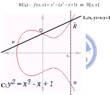
Consider the following algebraic curve in affine space: I(CR) : f x y( , )=y2−(x3− + in [ , ]x 1) x y

Figure 2.1

An elliptic curve C and rational function L1 over

The algebraic closure of is the field of the complex numbers; we still denote it as

K .

The affine variety over K is given by ( ) {( , ) | ,I C = x y x y∈K f x y, ( , ) 0}= . The coordinate ring of C is given by the quotient ring :

(

2 3

)

[ ] [ , ]/ ( 1) K C =K x y y − x − +x . P Q R

R

x3 L1(x, y)=x-y+1

C:

(25)

The function field of C is given by: K C( ) g| ,g h K C[ ]

h

⎧ ⎫

=_⎨ ∈ _⎬

⎩ ⎭.

The line through the point P, Q is a rational function given by L1(x, y).

1

( ) 3 ( ) ( ) ( )

div L = + + − ∞ =P Q R P− ∞ + Q− ∞ + R− ∞ .

The vertical line through R and R is a rational function given by L2(x, y)=x-x3.

2

( ) 2 ( ) ( )

div L = + − ∞ =R R R− ∞ + R− ∞ .

Let D₁= − ∞ , P D₂ = − ∞ and Q D₃ = − ∞ in the Jacobian J = DR 0/P, we have :

(

1 2

)

3 1 2 1 2 ( ) ( ) ( ) ( ) ( ) D D D P Q R div L div L L div P L + − = − ∞ + − ∞ − − ∞ = − ⎛ ⎞ = _⎜ _⎟∈ ⎝ ⎠

Hence D1+D2~D3, the Jacobian group law is the same as point addition on an elliptic

(26)

Chapter 3 Hyperelliptic Curves

Hyperelliptic curve is a kind of algebraic curve, and elliptic curve is a special case of hyperelliptic curve. In chapter 2, we defined the function field of an algebraic curve. The Jacobian is the group of degree zero divisors modulo principal divisors, i.e. the quotient group J = D0

/P over an algebraic closed field K . Since

the implementation of arithmetic on a hyperelliptic curve works with the base field K, we need to know the definitions over K.

Let C be a hyperelliptic curve defined over a finite field K. Let P = (x, y) ∈C, and let σ be an automorphism of K over K which means σ is an isomorphism from

K to itself and σ(x) = x for all x ∈K. Then Pσ : ( ,= xσ yσ) is also a point on C,

and ∞ = ∞ . σ

Definition 3.1 (Field of definition of a divisor)

A divisor D=

∑

m P_P is said to be defined over K if Dσ :=

∑

m P_P σ is equal to

D for all automorphisms of K over K.

Notice that the set of all automorphisms of K over K is the Galois Group

(

/

)

Gal K K defined in Definition 2.10 (Galois Group).

If a divisor D is defined over K, it does not mean that each point in the support of D is a K-rational point. A principal divisor is defined over K if and only if it is a

(27)

divisors defined over K in J is a subgroup of J.

Since each element of the Jacobian is a coset, we need a unique representation for the divisors in the Jacobian. Such divisors exist and are called reduced divisor, which is introduced in section 3.2. In section 3.3, we introduce the Mumford’s representation [27]: a reduced divisor can be represented by the gcd of two polynomials a(x) and y- b(x). The points associated to the corresponding divisor are the roots of both a(x) and y- b(x). These two polynomials can also be seen as ideals modulo principal ideals. The equivalence classes are called ideal classes. Adding divisors in the Jacobian is the same as composing ideals. Cantor’s algorithm [2] can efficiently compute the group operation of two divisors in the Jacobian.

3.1 Definitions and properties

We use K to denote a field and K to denote the algebraic closure of K in this chapter.

Definition 3.2 (Hyperelliptic curve)

A hyperelliptic curve of genus g over K is an equation of the form C: 2 _{( )} _{( )}

y +h x y= f x in K[x, y], where deg(h(x)) ≦ g, deg(f(x)) = 2g+1, f(x) is a

monic polynomial, and the integer g ≧ 1. A hyperelliptic curve C should be

non-singular, that is, there are no solutions (x, y)∈ × on curve C which satisfy K K

both partial derivative equations 2y+h x( ) 0= and '( )h x y− f x'( ) 0= .

Definition 3.3 (K-rational points)

The set _{( )}

{

_{( , ) | ,} _, 2 _{( )} _{( )}

}

_{{ }}

(28)

K-rational points on C. The point ∞ is called the point at infinity.

Definition 3.4 (Opposite, special and ordinary points)

For P=(x, y) ∈C the opposite of P is the point P=( ,x − −y h x( )). If P= P then it is called special point, otherwise it is called ordinary. The opposite of the point at infinity ∞ is defined as ∞ = ∞ , hence is a special point.

Lemma 3.1

Let C: 2 _{( )} _{( )}

y +h x y= f x be a hyperelliptic curve defined over K. If the

characteristic of K is odd, then C can be transformed to the form 2

1( )

y = f x where f1(x) has no repeated roots in K .

Proof:

Under the change of variables xÆx, yÆ(y-h(x)/2), the equation of C is transformed to ₍ ( )₎2 _{( )(} ( )₎ _{( )} 2 2 h x h x y− +h x y− = f x , which simplifies to 2 2 1 ( ) ( ) ( ) 4 h x y = f x + = f x .

Since C is a hyperelliptic curve, there is no point (x, y) K K∈ × satisfying

y2=f1(x), 2y=0, and f1’(x) =0. Therefore, f1(x) has no repeated roots.

Lemma 3.2

The polynomial _{( , )} 2 _{( )} _{( )}

F x y = y +h x y− f x is irreducible over K . Proof:

Suppose F(x, y) is reducible over K , then ( , ) (F x y = y−a x( ))(y b x+ ( ))

2 _{( ( )} _{( ))} _{( ) ( )}

y b x a x y a x b x

= + − − for some a, b∈K x[ ]. But deg(a(x)b(x)) = deg(f(x)) = 2g+1 and deg(a(x)+b(x)) = deg(h(x)) ≦g which is impossible.

(29)

3.2 Reduced divisors

We defined the Jacobian of curves in chapter 2, and with the definitions in section 3.1, we know that the Jacobian of a hyperelliptic curve C is J = D0

/P. Note that two

divisors D1 and D2 in J are said to be equivalent if they are in the same equivalence

class, i.e. D1-D2∈P, denoted by D1~D2. In the following we introduce reduced

divisor to uniquely represent the divisors in the same equivalence class of J.

Definition 3.5 (Semi-reduced divisor)

A semi-reduced divisor is a degree zero divisor of the form

\ \

P P

P C P C

D m P m

∈ ∞ ∈ ∞

=

∑

−

∑

∞ with the following properties: (i) mP>0,

(ii) if P P and m >0 then m =0≠ _P _P , (iii) if P P and m >0 then m =1= _P _P .

Definition 3.6 (Reduced divisor)

Let \ \ P P P C P C D m P m ∈ ∞ ∈ ∞ =

∑

−

∑

∞ be a semi-reduced divisor. If \ P P C m genus ∈ ∞ ≤

∑

then D is called a reduced divisor.

Lemma 3.3

For each divisor D∈D0_{there exists a semi-reduced divisor D}

1∈D0 such that

D~D1.

(30)

Let \ P P C D m P m ∈ ∞

=

∑

− ∞. Let (C1, C2, C3) be the partition of the support of D,

such that C₁={P∈C\ |∞ P≠P m, _P ≥m_P}, C₂ ={P∈C\ |∞ P≠P m, _P ≥m_P} , and C₁ ={P∈C\ |∞ P=P}. Then 1 2 3 P P P P C P C P C D m P m P m P m ∈ ∈ ∈ =

∑

+

∑

+

∑

− ∞. Let 2 3 1 ( , ) ( , ) ( ) ( ) 2 P P P P P P P P P x y C P x y C m D D m div x x div x x = ∈ = ∈ ⎢ ⎥ = − ⋅ − − _⎢ _⎥⋅ − ⎣ ⎦

∑

1 3 1 ( ) ( 2 ) 2 P P P P P C P C m m m P m P m ∈ ∈ ⎢ ⎥ = − + − ⋅_⎢ _⎥ − ∞ ⎣ ⎦

∑

for some m₁∈ . Z

Hence D1~D and D1 is semi-reduced.

For example, let 0

1 1 2 6 4 3 13 D= P+ P + P − ∞ ∈D where P₁≠P₁ and P₂ =P₂ . Then C1={P1}, C2={P₁}, and C3={P2}. Let 1 2 1 3 4 ( ) ( ) 2 P P D = − ⋅D div x−x −⎢ ⎥_{⎢ ⎥}⋅div x−x ⎣ ⎦ , then D1~D. 1 4( 1 1 2 ) (2 2 2 ) 2 1 2 3 D = −D P+ − ∞ −P P − ∞ = P+P − ∞. Hence D1 is semi-reduced.

Theorem 3.1 [25]

For each divisor D∈D0_{there exists a unique reduced divisor D}

1 such that D~D1.

3.3 Representation

When we implement a hyperelliptic curve cryptosystem, we work over a finite field K. In the following, we introduce the computational representation of reduced divisors of the Jacobian defined over K, which is so-called Mumford representation [27].

(31)

Fact 3.1 (Mumford representation)

For a hyperelliptic curve C: 2 _{( )} _{( )}

y +h x y= f y in K x y[ , ] , and ( , ) ( ) i i i i i i P x y C D m P m = ∈

=

∑

−

∑

∞ be a semi-reduced divisor, we can use two polynomials a(x), b(x) ∈K x[ ] to uniquely represent D. Let ( ) ( )mi

i

a x =

∏

x−x .

Let b(x) be the unique polynomial satisfying: (i) degx(b) < degx(a),

(ii) b(xi) = yi for all i which mi ≠0,

(iii) a(x) divides ( _{( )}2 _{( ) ( )} _{( )}

b x +b x h x − f x ).

Then D = gcd(div(a(x)), div(b(x)-y)); we usually simplify the notation as div(a, b).

If D=div(a, b) is a reduced divisor, then deg ( )_x a =

∑

m_i ≤genus.

The zero divisor, the identity of JC(K), is represented by div(1, 0). The

opposite of a divisor div(a, b) is given by div(a, -h-b), which is also called involution. This means div(a, b) + div(a, -h-b) ~ div(1, 0) under the Jacobian group law.

Fact 3.2 (Hasse-Weil Bound)

Let C be a hyperelliptic curve of genus g defined over Fq. Then the bound of

the order of JC(Fq) is given by:

(

)

2

(

)

2

1 g # C( )q 1 g

q− ≤ J F ≤ q+ ,

and the number of Fq-rational points is:

1 2 # ( )q 1 2

q+ − g q≤ C F ≤ + +q g q.

As a result, we know that # ( ) g C q

(32)

3.4 Group law

By using Mumford representation described in the previous section, Cantor’s algorithm [2] can compute the group operation of JC(K) efficiently.

Algorithm 3.1 (Cantor’s algorithm)

Input: Reduced divisors D1 = div(a1, b1) and D2=div(a2, b2) ∈JC(K).

Output: The reduced divisor D3 = div(a3, b3) sucht that D3 ~ D1+D2.

Phase 1: (Composition)

1. Compute d1 = gcd(a1, a2) = e1a1 + e2a2

2. Compute d = gcd(d1, b1+b2+h) = c1d1 + c2( b1+b2+h)

3. Let s1 = c1e1, s2 = c1e2, and s3 = c2, so that

d = s1a1 + s2a2 + s3( b1+b2+h) 4. Set 1 2 2 a a a d = and _b s a b1 1 2 s a b2 2 1 s b b3( 1 2 f) _mod_a d + + + = Phase 2: (Reduction) 5. Set 2 ' f bh b a a − − = and ' (b = − −h b) mod a

6. If deg( ')a > then set g a←a', b←b' and go to step 5.

7. Make a' monic, and output (a3, b3) = ( ', ')a b .

In Cantor’s algorithm, the composition phase gives a semi-reduced divisor div(a, b) ~ D1+D2, and the reduction phase reduces a semi-reduced divisor to the

(33)

Example 3.1

Let C: y2+y = x5+1 be a hyperelliptic curve of genus 2 over finite field F2.

Given D1=div(x+1, 0) and D2=div(x2+1, x)∈JC(F2).

d = gcd(a1, a2, b1+b2+h) = gcd(x+1, x2+1, x+1) = x+1 ⇒ s1=1, s2=s3=0.

(

)

(

)

(

)

2 1 2 2 2 1 1 1 1 x x a a a x d x + + = = = + + .

(

)

1 1 2 2 2 1 3( 1 2 ) _mod1 _mod_(x+1)=1 1 x x s a b s a b s b b f b a d x + + + + = = + .

Since deg(a)=1≦2, the divisor div(a, b) is already reduced. Then, we have D1+ D2 = div(x+1, 0) + div(x2+1, x) = div(x+1, 1).

In recent years, several researchers have derived the explicit formulas for small genus hyperelliptic curves from Cantor’s algorithm. They investigate what can be the input of Cantor’s algorithm and proceed in considering these different cases. With careful analysis, some redundant field operations can be omitted in explicit formulas. For example, Lange [22] presents explicit formulas for the group law of genus 2 hyperelliptic curves, and the most common case in the addition of two reduced divisor requires 1 inversion, 12 multiplications, and 2 squarings. The

explicit formulas for genus 3 hyperelliptic curves can be found in [17]. When genus becomes higher than 4, the explicit formulas is getting too complicated and may not be possibly derived by hand.

3.5 Hyperelliptic curve discrete log problem

(HCDLP)

The security of several cryptosystems is related to the difficulty of computing discrete logarithms modulo a large prime number p; i.e. given two numbers (g mod p) and (gx mod p), it seems to be infeasible to compute x when p is large enough. Instead of using the DLP modulo a large prime p as the basis of cryptographic protocols, one can consider the DLP in an arbitrary group that admits an efficient

(34)

element representation and group law.

Definition 3.7 (DLP)

Let G be a finite cyclic group G= <g> of order n, and given an element h∈G.. The discrete logarithm problem is to find the integer x∈[0, n-1], such that gx_=h.

Since the Jacobian of a hyperelliptic curve is also a finite abelian group, based on the difficulty of the DLP, it can be designed for cryptographic use.

Definition 3.8 (HCDLP)

Let C be a hyperelliptic curve over a finite field Fq and JC(Fq) its Jacobian with

order # JC(Fq) = n. Given two reduced divisors D1, D2∈JC(Fq) and D2∈<D1>.

The hyperelliptic curve discrete logarithm problem is to find the integer λ∈[0, n-1], such that λD1=D2.

Example 3.2

Consider the genus 2 hyperelliptic curve: C: y2 = x5 + 2x4 + 1 in F3[x, y]. The

partial derivatives are 2x4 + 2x3=0 and 2y=0. Since there are no points in F F× which satisfy C and the partial derivatives, the hyperelliptic curve is non-singular.

Although the divisors are defined over F3, the points in the support of a divisor are

in F . ₃2

The finite field 2

2 3

3 [ ]/( 1) {0,1 , 2 ,1 2 , 2, 2 2 , , 2 ,1} F ≅F x x + = +i i + i + i i +i .

The F -rational points are P₃2 1 = (0, 1), P2 = (1, 2), P3 = (1, 1), P4 = (0, 2),

P5 = (2+i, 2+2i), P6 = (2+2i, 2+i), P7 = (i, 2+i), P8 = (2i, 2+2i),

P9 = (i, 1+2i), P10 = (2i, 1+i), P11 = (2+i, 1+i), P12 = (2+2i, 1+2i), ∞.

The order of Jacobian #JC(F3) = 17.

(35)

Cantor’s algorithm to generate the group elements. 1 D1 = div(x2, 1) = P1 + P1 - 2∞ 2 D1 = div(x+2, 2) = P2 - ∞ 3 D1 = div(x2+2x+2, 2x+1) = P5 + P6 - 2∞ 4 D1 = div(x2+x+1, x+1) = P2 + P2 - 2∞ 5 D1 = div(x2+1, x+1) = P9 + P10 - 2∞ 6 D1 = div(x2+2x, 2x+2) = P3 + P4 - 2∞ 7 D1 = div(x2+2x, 1) = P1 + P3 - 2∞ 8 D1 = div(x, 2) = P4 - ∞ 9 D1 = div(x, 1) = P1 - ∞ 10D1 = div(x2+2x, 2) = P2 + P4 - 2∞ 11D1 = div(x2+2x, x+1) = P1 + P2 - 2∞ 12D1 = div(x2+1, x+2) = P7 + P8 - 2∞ 13D1 = div(x2+x+1, 2x+2) = P3 + P3 - 2∞ 14D1 = div(x2+2x+2, x+2) = P11 + P12 - 2∞ 15D1 = div(x2+2, 1) = P3 - ∞ 16D1 = div(x2, 2) = P4 + P4 - 2∞ 17D1 = div(1, 0)

(36)

Chapter 4 Algorithms for HCDLP

4.1 Introduction

The best known algorithm for solving the DLP in generic groups is Pollard’s rho algorithm. Pollard’s algorithm has an exponential expected running time of

2

n

π group operations and negligible storage requirements. In order to prevent such square-root attacks, the group order n must have a large prime factor. There are faster algorithms for the DLP than Pollard’s rho method. The most powerful is the index calculus method which yields subexponential-time algorithms for the DLP in some groups.

The first subexponential-time algorithm to compute discrete logarithms over hyperelliptic curves of large genus is introduced by Adleman, DeMassais and Huang [1] in 1994. This algorithm was rather theoretical, and some improvements on it were done by other researchers. Flassenberg and Paulus [9] implemented a sieve version of this algorithm, but the consequence for cryptographical applications is not clear. Enge [6] improved the original algorithm and gave a precise evaluation of the running time, but did not implement his ideas. Muller, Stein and Thiel [26] extended the resultsto the real quadratic congruence function fields. Smart and Galbraith [12] also gave some ideas in the context of the Weil descent, following ideas of Frey; they dealt with general curves (not hyperelliptic). We will not discuss those in details but list them as references.

(37)

When the index calculus algorithm is applied on the small genus HCDLP, even the fastest variation is not faster than Pollard’s rho method for the genus less than 3. Hence the use of hyperelliptic curves in public-key cryptography appears as an alternative to the use of elliptic curves, with the advantage that it can be used in a smaller base field for the same level of security. In order to analyze the security of such systems, we need to know how the index calculus method works for solving small genus HCDLP.

In 2000, Gaudry [13] first presented a variation of index calculus attack for a hyperelliptic curve of genus g over Fq that could solve the HCDLP in time O q( )2 .

And Harley [13] improved this algorithm with reduced factor base such that HCDLP can be solved in time

2 2 1 g O q − + ⎛ ⎞ ⎜ ⎟ ⎜ ⎟

⎝ ⎠. Furthermore, Thériault improved it by using the almost-smooth divisor which contains exactly one large prime. Theriault’s algorithm [32] works in time

4 2 2g 1 O q − + ⎛ ⎞ ⎜ ⎟ ⎜ ⎟ ⎝ ⎠.

By considering double large prime, the time complexity of hyperelliptic index calculus algorithm can be reduced to

2 2 g O q − ⎛ ⎞ ⎜ ⎟ ⎜ ⎟

⎝ ⎠ . This idea was proposed independently by Gaudry et al. [16] and Naogo [28] in 2004. They used different tricks to handle large primes, but got the same time complexity. We discuss these variations of index calculus algorithm for small genus HCDLP in section 4.2.

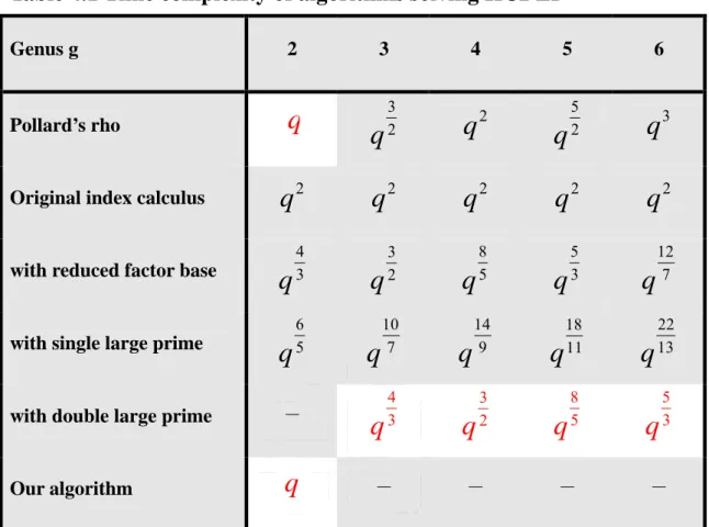
However, the double large prime variation can not be applied on genus 2 hyperelliptic curves. We propose an algorithm that can solve the genus 2 HCDLP with time complexity O(q) in Chapter 5 which can be comparable to Pollard’s rho method. Table 4.1 shows the comparison between these algorithms described above. Our algorithm has the same time complexity as Pollard’s rho method but smaller

(38)

hiding constant term. We also have detailed analysis in Chapter 5.

Table 4.1 Time complexity of algorithms solving HCDLP

Genus g 2 3 4 5 6 Pollard’s rho

q

3 2

q

2 5 2

q

3

Original index calculus

q

2

q

2

q

2

q

2

q

2

with reduced factor base

4 3

q

3 2

q

8 5

q

5 3

q

12 7

q

with single large prime

6 5

q

10 7

q

14 9

q

18 11

q

22 13

q

with double large prime －

4 3

q

3 2

q

8 5

q

5 3

q

Our algorithm

q

－－－－

4.2 Index calculus algorithm for small genus HCDLP

A reduced divisor in the Jacobian JC(K) is represented by two polynomials (a, b),

and the factorization of a as polynomial in K[x] is compatible with the Jacobian group law. This is the key stone for defining a smooth divisor and then the index calculus algorithm.

Fact 4.1 (Factorization)

Let C be a hyperelliptic curve over a finite field Fq. Let D=div(a, b) be a

(39)

irreducible factors of a(x) in Fq[x]. Let bi(x) = b(x) (mod ai(x)).

Then Di = div(ai, bi) is a reduced divisor and D=D=

∑

Di in JC(Fq).

Remark 4.1

To factor polynomials over finite fields we can use the Cantor-Zassenhaus algorithm, which is invented by D. Cantor and Hans Zassenhaus in 1981 [3]. It is currently implemented in many well-known computer algebra systems.

With this result in Fact 4.1, a reduced divisor can be rewritten as the sum of reduced divisors of smaller deg(ai), and deg( )a =

∑

deg( )ai . If the a-polynomial of a reduced divisor D is irreducible then it can not be rewritten as their decomposition. We call them primes in JC(Fq).

Definition 4.1 (Prime)

A reduced divisor D=div(a, b) ∈ JC(Fq) is said to be prime if the polynomial a

is irreducible in Fq[x].

Definition 4.2 (B-smooth)

Let B be an integer. A divisor is said to be B-smooth if all the prime divisors in its factorization of a-polynomial have degree at most B. When B= 1, a 1-smooth divisor will be a divisor for which the polynomial a splits completely over Fq.

We give a sketch of the index calculus algorithm in the following. Several improvements described in this section are based on this algorithm.

(40)

Algorithm 4.1 Hyperelliptic index calculus algorithm

Input: A divisor D1 in JC(Fq) with know order n = ord(D1),

and a divisor D2∈<D1>.

Output: An integer λ sucht that D2=λD1.

1. Fix smoothness bound B and construct the factor base F. 2. While not enough relations have been found do:

Pick a random element R=αD1+βD2.

If R is smooth, record the corresponding relation. 3. Solve the linear algebra system over Zn.

4. Return λ.

The factor base F contains all the prime reduced divisors which a-polynomial has degree at most B: F ={D∈JC( ) :Fq D=div a b is prime( , ) , deg( )a ≤B} . For convenience, we use gi for i=1,2,…,#F to denote the element in F. To find all the

prime divisors in F, it suffices to test all the monic polynomial a(x) of degree at most B, checking if it is irreducible and if there exists a polynomial b(x) such that

div(a, b)∈JC(Fq).

While searching the smooth relations in step 2, a naive way to select a random element R=αD1+βD2 is costly: two integers α and β are randomly chosen in [0, n-1]

and then two scalar multiplications have to be done. It costs O(log n) group operations. We can use a pseudo random walk instead, so that each new random element R costs just one group operation.

Let R₀ =α₀D₁+β₀D₂ be the starting point of the walk where α0 and β0 are

random integers in [0, n-1]. For j from 1 to r, we compute random divisors

(41)

The index j∈[1, r] is given by a hush function H evaluated at Ri. In other words,

Ri+1=Ri+Tj where j=H(Ri)∈ [1, r], and αi+1=αi +aj, βi+1 = βi+ bj. Once the

initialization is finished, we can compute a new pseudo-random element Ri+1 at the

cost of one addition in the Jacobian. Practical experiments suggest that by taking r= 20 the pseudo random walk behaves almost like a purely random walk.

For each Ri of the random walk, test its smoothness by factoring the

a-polynomial of Ri. If all its irreducible factors have degree at most B (then it is

smooth), express it on the factor base; otherwise, throw it away. Thus we collect a subsequence of the sequence (Ri) where all the divisors are smooth. We denote this

subsequence by (Sk) with kth smooth element Sk=αkD1+βkD2. Hence we can put the

result of this computation in a matrix M, each column representing an element of the factor base, and each row being a reduced divisor Sk expressed on the basis: for a row

k, we have ₁ ₂ 1 # k ki i k k i F S m g α D β D ≤ ≤

=

∑

= + , where M = (mki). We collect #F + 1 rows

in order to have a (#F+ ×1) #F matrix. Thus the kernel of the transpose of M is of

dimension at least 1.

Using linear algebra, we find a non-zero vector (γk) of this kernel, which

corresponds to a relation between the Sk’s. So that

(

) (

1

)

2

0

k k k k k k

kγ S = = kγ α D + kγ β D

∑

, and then _k k k (mod )

k k k n γ α λ γ β = −

∑

. The

discrete logarithm is now found with high probability, because the denominator is zero with probability 1

n.

In this algorithm, there are two crucial points: one is to search enough smooth relations, and another is to solve the large linear system. In the matrix obtained in the algorithm, each row is a smooth divisor written as sum of at most g elements of the factor base. Hence the matrix is very sparse, and we have at most g terms in

(42)

each row. For such a sparse matrix, Lanczos’s [21] or Wiedemann’s [33][5] algorithm can be used, in order to get a solution in time quadratic in the number of rows, instead of cubic by Gaussian elimination.

We know that the index calculus algorithm can solve HCDLP in a subexponential time 1, 2 2 g q O L⎛_⎜ ⎛_⎜ ⎞_⎟⎞_⎟ ⎝ ⎠

⎝ ⎠ when g logq [1], where

(

) (

)

(

1

)

( , ) exp log log log

N

L α c = c N α N −α . When the genus is relatively small (say at

most 9), the theoretical optimal smoothness bound log 1, 2 2 g q q B=⎡_⎢ L ⎛_⎜ ⎞_⎟⎤_⎥ ⎝ ⎠ ⎢ ⎥ which

tends to 0. In this case, B= 1 is the best choice. The first index calculus algorithm for hyperelliptic curve of small genus was proposed by Gaudry in 2000. We summarize in the following algorithm.

Algorithm 4.2 Index calculus algorithm for small genus HCDLP

Input: A hyperelliptic curve C of small genus g over Fq,

a divisor D1 in JC(Fq) with know order n = ord(D1),

and a divisor D2∈<D1>.

Output: An integer λ sucht that D2=λD1.

1. /* Build the factor base F */

For each monic irreducible polynomial ai over Fq of degree 1, try to find bi such

that div(ai, bi) is a divisor of the curve. If there is a solution, store gi =div(ai, bi)

in F.

2. /* Initialization of the random walk */

For j from 1 to 20, select aj and bj at random in [0, n-1], and compute

Tj := ajD1 + bjD2.

(43)

Set k to 1. 3. /* Main loop */

(a) /* Look for a smooth divisor */

Compute j := H(R0), R0 := R0 + Tj, α0 := α0 + aj mod n, andβ0 := β0 + bj mod n.

Repeat this step until R0 is a smooth divisor.

(b) /* Express R0 on the factor base F */

Factor a0(u) over Fq, and determine the positions of the factors in the basis G..

Store the result as a row Rk =

∑

m gki i of a matrix M = (mki). Store the coefficients αk = α0 and βk = β0.

If k < #F + 1, then set k := k + 1, and return to step 3.a. 4. /* Linear algebra */

Find a non-zero vector (γk) of the kernel of the transpose of the matrix M.

The computation can be done in Zn.

5. /* Solution */ Return _k k k (mod ) k k k n γ α λ γ β = −

∑

.

Lemma 4.1

The proportion of smooth divisors in the Jacobian of a curve of genus g over Fq

tends to 1 !

g .

Proof:

By the Hasse-Weil bound, #F= #C(Fq) = O(q) and #JC(Fq) = O(qg). The

smooth divisors can be written as the sum of at most g points in C(Fq), hence we have

about

!

g

q

g smooth divisors in JC(Fq). The proportion is

1 !

g .

(44)

Fq. Step 2 requires a constant number of Jacobian operations. Step 3 is a loop of

O(q) times to find enough smooth relations. In step 4, this linear algebra step consists in finding a vector of the kernel in a sparse matrix of size O(q), and of weight O(gq); the coefficient are in Zn. Hence Lanczos's algorithm provides a solution with

cost O(gq2). This last step requires only O(q) multiplications modulo n, and one inversion. When q is large, we can regard g and logq as small constant. Then the complexity of this algorithm is O(q2).

Theorem 4.1 [13]

Let C be a hyperelliptic curve of genus g over the finite field Fq. If q>g! then

the discrete logarithms in JC(Fq) can be computed in expected time O g q

(

3 2+ε

)

.

Example 4.1

Given a genus 2 hyperelliptic curve C: y2 = x5 + 2x4 + 1 over F3. This curve is

also used as an example in Example 3.2. Let D1 = div(x2, 1) with ord(D1) = 17, and

D2 = div(x2+1, x+2) ∈<D1>. We can use the index calculus algorithm described in

Algorithm 4.2 to find an integer λ such that D2=λD1.

1. Construct factor base

F = {g1=div(x, 1), g2=div(x+2, 2), g3=div(x+2, 1), g4=div(x, 2)}.

2. Initialize the pseudo-random walk: T1 = 2D1+ 10D2 = div(x2+2x+2, 2x+1)

T2 = 13D1 + 5D2 = div(x2+1, x+1)

T3 = 3D1 + 7D2 = div(x+2, 2)

3. Search enough smooth relations by using a pseudo random walk: R0 = 1D1+1D2 = div(x2+x+1, 2x+2) = 2g3.

R1 = R0+T2 =14D1+6D2 = div(x2, 1) = 2g1.

R2 = R1+T1 =16D1+16D2 = div(x2+x+1,x+1) = 2g2.

R3 = R2+T1 = 1D1+9D2 = div(x2+2x, 1) = g1+g3.

R4 = R3+T3 = 4D1+16D2 = div(x,1) = g1.

(45)

These smooth relations are stored in a matrix M:

4. When there is enough(#F+1 = 5) smooth relations, we can find a non-trivial kernel r of M, such that rM=0. We have r =(0, 1, 0, 0, -2)T.

2 1 0 0 0 0 0 0 0 2 0 0 0 0 0 0 r M ⎡ ⎤ ⎡ ⎤ ⎡ ⎤ ⎢ ⎥ ⎢ ⎥ ⎢ ⎥ ⎢ ⎥ ⎢ ⎥ ⎢ ⎥ ⋅ = + + + − ⋅ = ⎢ ⎥ ⎢ ⎥ ⎢ ⎥ ⎢ ⎥ ⎢ ⎥ ⎢ ⎥ ⎣ ⎦ ⎣ ⎦ ⎣ ⎦ 14 4 6 0 0 0 2 6 16 26 i i r α β ⎡ ⎤ ⎡ ⎤ ⎡ ⎤ ⎡ ⎤ ⇒ ⋅_{⎢ ⎥}= +_{⎢ ⎥}+ + − ⋅_{⎢ ⎥ ⎢}= _⎥ − ⎣ ⎦ ⎣ ⎦ ⎣ ⎦ ⎣ ⎦ Hence, 6D1-26D2 = 0, 2 1 1 D = [6/26 (mod 17)] D =12D ⇒ .

4.2.1 Reduced factor base

Because the running time for Gaudry’s algorithm is dominated by the cost of solving the linear algebra, a natural approach to improve the algorithm is to reduce the cost of linear algebra part. Hence we need to reduce the size of the linear system, which means reducing the size of factor base. This was first introduced by Robert Harley. We can choose the factor base F with |F|=qr where r is a real number in the interval (0, 1). This increases the cost of searching relation, because it also reduces the proportion of the smooth divisors in the Jacobian. To balance the cost of the relation search and linear algebra

1

g r

g

≈

+ is the best choice. Then, the time αi βi g1 g2 g3 g4 Matrix M 4 16 1 0 0 0 1 1 0 0 2 0 14 6 2 0 0 0 16 16 0 2 0 0 1 9 1 0 1 0

(46)

complexity of the index calculus algorithm with reduced factor base is 2 2 1 g O q − + ⎛ ⎞ ⎜ ⎟ ⎜ ⎟ ⎝ ⎠.

Theorem 4.2 [13]

the discrete logarithms in JC(Fq) can be computed in expected time

2 2 5 g 1 O g q ε − + + ⎛ ⎞ ⎜ ⎟ ⎜ ⎟ ⎝ ⎠.

4.2.2 Single large prime variation

As the index calculus algorithm for the multiplicative group of a finite field, the hyperelliptic index calculus algorithm can be improved by using large primes.

Definition 4.3 (Large prime)

Let r be a real number such that 0<r<1. A subset S of Fq of size qr is fixed

arbitrarily. The factor base F is the set F ={P=( , )x y ∈C F( )q ⊂JC( );Fq x∈S}. The set of large primes L is the set L={P∈C F( )q ⊂JacC( )} \Fq F.

We have # r

F ≈ and # L qq ≈ . The union of factor base and large primes is

the set of Fq-rational points (xi, yi) ∈C(Fq) which can represent the prime divisors

with div(ai, bi) = div(x-xi, yi).

Definition 4.4 (1-almost smooth divisor)

A reduced divisor D=

∑

m P_i _i− ∞m is said to be 1-almost smooth if all but

(47)

Definition 4.5 (2-almost smooth divisor)

A reduced divisor D=

∑

m P_i _i− ∞m is said to be 2-almost smooth if all but

exactly two of the Pi’s are in F and the remaining Pi’s are two large primes.

Simple combinatorial arguments give good estimates for the probabilities of obtaining almost smooth divisors in the relation search.

Lemma 4.2

The probability for a random divisor to be smooth is approximately

( 1) ! g r q g − . The probability for a random divisor to be 1-almost smooth is approximately

( 1)( 1) ( 1)! g r q g − −

− . The probability for a random divisor to be 2-almost smooth is

approximately ( 2)( 1) 2( 2)! g r q g − − − .

We now consider the single large prime variation of the index calculus algorithm. In order to take advantage of the high number of 1-almost smooth divisors, we must find pairs of these divisors with the same large prime. For example, given two 1-almost smooth divisors 1 1 *

i i i P F D m P n Q ∈ =

∑

+ − ∞, 2 2 * i i i P F D m P n Q ∈ =

∑

+ − ∞ where Q is a large prime, then we can obtain a smooth divisor by computing n D2 1−n D1 2.

The following algorithm shows how this method can be applied in the relation search of the original index calculus algorithm.

Algorithm 4.4.5: Searching relation with single large prime

Input: A hyperelliptic curve C of small genus g over Fq,

(48)

a divisor D2∈<D1>,

a factor base F, and the set of large primes L.

Output: A system of k smooth divisors of the form R_i =α_iD₁+β_iD₂.

1. /* Initialization of the random walk */

For j from 1 to 20, select aj and bj at random in [0, n-1], and compute

Tj := ajD1 + bjD2.

Select α and β at random in [0, n-1] and compute R:= αD1 +βD2.

PÅ{} iÅ1

2. /* Main loop */ While i k do{≦

RÅR+Tj for some randomly chosen j, update α and β.

Decompose R into prime divisors If R is smooth then

RiÅR

iÅi+1

If R is 1-almost smooth with a large prime Q then If Q is already in P then

Obtain a smooth divisor R by cancelling the large prime Q RiÅR

iÅi+1

else (Q is not in P)

Add Q to the set P with the associated relation R }

(49)

According to Theriault’s analysis, by choosing the factor base F such that 1 1 / 2 2 2 | |F O g q g g ε ⎛ ₋ ⎞ ⎛ ₊ ⎞₊ ⎜ ⎟ ⎜ ⎟ ⎝ ⎠ ⎝ ⎠ ⎛ ⎞ = ⎜_⎜ ⎟_⎟

⎝ ⎠, we get the following result:

Theorem 4.3 [32]

the discrete logarithms in JC(Fq) can be computed in expected time

4 2 5 2g 1 O g q ε − + + ⎛ ⎞ ⎜ ⎟ ⎜ ⎟ ⎝ ⎠.

Example 4.2

Given the same HCDLP as in Example 4.1. Let C: y2_{= x}5_{+ 2x}4_{+ 1 over F}

3.

D1 = div(x2, 1) with ord(D1) = 17, and D2 = div(x2+1, x+2) ∈<D1>. We want

to find an integer λ such that D2=λD1.

1. Construct factor base F = {g1=div(x, 1), g2=div(x+2, 2), g3=div(x+2, 1)}, and

the set of large primes is {g4=div(x, 2)}.

2. Initialize the pseudo-random walk: T1 = 2D1+ 10D2 = div(x2+2x+2, 2x+1)

T2 = 13D1 + 5D2 = div(x2+1, x+1)

T3 = 3D1 + 7D2 = div(x+2, 2)

3. Search enough smooth relations by using a pseudo random walk: R0 = 16D1+8D2= div(x2+2x, 2) = g2+g4.

R1 = R0+T1 = 1D1+1D2 = div(x2+x+1, 2x+2) = 2g3.

R2 = R1+T2 = 14D1+6D2 = div(x2,1) = 2g1.

R3 = R2+T2 = 10D1+11D2 = div(x2+2x, 2x+2) = g3+g4.

R4 = R3+T2 = 6D1+16D2 = div(x2+2x, x+1) = g1+g2.

R0 and R3 are 1-almost smooth relations with the same large prime g4. We

can calculate a smooth relation R’= R0-R3=6D1-3D2=g2-g3.

(50)

4. When there is enough(#F+1 = 4) smooth relations, we can find a non-trivial kernel r of M, such that rM=0. We have r =(1, 1, 2, -2)T.

0 2 0 1 0 0 0 2 1 2 1 0 2 0 1 0 0 r M ⎡ ⎤ ⎡ ⎤ ⎡ ⎤ ⎡ ⎤ ⎡ ⎤ ⎢ ⎥ ⎢ ⎥ ⎢ ⎥ ⎢ ⎥ ⎢ ⎥ ⋅ =_{⎢ ⎥ ⎢ ⎥}+ + ⋅_{⎢ ⎥}− ⋅_{⎢ ⎥ ⎢ ⎥}= ⎢ ⎥ ⎢ ⎥ ⎢ ⎥− ⎢ ⎥ ⎢ ⎥ ⎣ ⎦ ⎣ ⎦ ⎣ ⎦ ⎣ ⎦ ⎣ ⎦ 1 14 6 6 15 2 2 1 6 3 16 31 i i r α β ⎡ ⎤ ⎡ ⎤ ⎡ ⎤ ⎡ ⎤ ⎡ ⎤ ⎡ ⎤ ⇒ ⋅_{⎢ ⎥ ⎢ ⎥ ⎢ ⎥}= + + ⋅_{⎢ ⎥}− ⋅_{⎢ ⎥ ⎢}= _⎥ − − ⎣ ⎦ ⎣ ⎦ ⎣ ⎦ ⎣ ⎦ ⎣ ⎦ ⎣ ⎦ Hence, 15D1-31D2 = 0, 2 1 1 D = [15/31 (mod 17)] D =12D ⇒ .

4.2.3 Double large prime variation

Since 1-almost smooth divisors can be used to produce relations so much faster, it is natural to also consider 2-almost smooth divisors. By the definition of 2-almost smooth divisor, the smallest genus g of a hyperelliptic curve is 3 such that a reduced divisor which is 2-almost smooth is of the form D=P+Q1+Q2-3∞ where P is in factor

base and Qi are large primes. Here is an example to cancel the large primes.

Example 4.3

Let C be a hyperelliptic curve of genus g=3. D1=P1+Q1+Q2-3∞,

D2=P2+Q2+Q3-3∞, and D3=P3+Q3+Q1-3∞ where Pi are in the factor base and Qi are

large primes. We can cancel the large primes by multiplying the divisors by a αi βi g1 g2 g3 Matrix M 1 1 0 0 2 14 6 2 0 0 6 -3 0 1 -1 6 16 1 1 0

超橢圓曲線密碼攻擊之研究

國

立

交

通

大

學

資訊科學與工程研究所

碩

士

論

文